temporal encoding of the input data in the network's hidden state space. This mixture is ... comprises a recurrent hidden layer (reservoir) with a large set of nonlinear neu- rons. ..... http://archive.ics.uci.edu/ml/index.html, 1998. [9] M. Forina and ...
Recurrence Enhances the Spatial Encoding of Static Inputs in Reservoir Networks Christian Emmerich, R. Felix Reinhart, and Jochen J. Steil Research Institute for Cognition and Robotics (CoR-Lab), Bielefeld University, Universit¨ atsstr. 25, 33615 Bielefeld, Germany {cemmeric,freinhar,jsteil}@cor-lab.uni-bielefeld.de http://www.cor-lab.de
Abstract We shed light on the key ingredients of reservoir computing and analyze the contribution of the network dynamics to the spatial encoding of inputs. Therefore, we introduce attractor-based reservoir networks for processing of static patterns and compare their performance and encoding capabilities with a related feedforward approach. We show that the network dynamics improve the nonlinear encoding of inputs in the reservoir state which can increase the task-specific performance. Key words: reservoir computing, extreme learning machine, static pattern recognition
1
Introduction
Reservoir computing (RC), a wellestablished paradigm to train recurrent neural networks, is based on the idea to restrict learning to a perceptron-like read-out layer, while the hidden reservoir network is initialized with random connection strengths and remains fixed. The latter can be understood as a “random, temporal and nonlinear kernel” [1] providing a suitFigure 1: Key ingredients of RC. able mixture of both spatial and temporal encoding of the input data in the network’s hidden state space. This mixture is based upon three key ingredients illustrated in Fig. 1: (i) the projection into a high dimensional state space, (ii) the nonlinearity of the approach and (iii) the recurrent connections in the reservoir. On the one hand, the advantages of a nonlinear projection into a high dimensional space are beyond controversy: so-called kernel expansions rely on the concept of a nonlinear transformation of the original data into a high dimensional feature space and the subsequent use of a simple, mostly linear, model. On the other hand, the recurrent connections implement a short-term memory by means of transient network states. Due to
2
Christian Emmerich, R. Felix Reinhart, and Jochen J. Steil
this short-term memory, reservoir networks are typically utilized for temporal pattern processing such as time-series prediction, classification and generation [2]. One could argue that a short-term memory could also be implemented in a more simple fashion, e.g. by an explicit delay-line. But we point out that the combination of spatial and temporal encoding makes the reservoir approach powerful and can explain the impressive performance on various tasks [3, 4, 5]. However, it remains unclear how the network dynamics influence the spatial encoding of inputs. Our hypothesis is that the dynamics of the reservoir network can enhance the spatial encoding of static inputs by means of a more nonlinear representation, which should consequently improve the task-specific performance. Moreover, we expect an improved performance when applying larger reservoirs, i.e. when using an increased dimensionality of the kernel expansion. Using attractor-based computation and by considering purely static input patterns, we systematically test the contribution of the network dynamics to the spatial encoding independently from its temporal effects. A statistical analysis of the distribution of the network’s attractor states allows to access the qualitative difference of the encoding caused by the network’s recurrence indepently of the task-specific performance.
2
Attractor-based Computation with Reservoir Networks
We consider the three-layered network architecture depicted in Fig. 2, which comprises a recurrent hidden layer (reservoir) with a large set of nonlinear neurons. The input, reservoir and output neurons are denoted by x ∈ D , h ∈ N and y ∈ C , respectively. The reservoir state is governed by discrete dynamics � h(t + 1) = f Winp x(t) + Wres h(t) , (1)
R
R
R
where the activation functions fi are applied componentwise. Typically, the reservoir neurons have sigmoidal activation functions such as fi (x) = tanh(x), whereas the output layer consists of linear neurons, i.e. y(t) = Wout h(t). Learning in reservoir networks is restricted to the read-out weights Wout . All other weights are randomly initialized and remain fixed. In order to infer a desired input-to-output mapping from a set of training examples (xTk , ykT )k=1,...,K , the read-out weights Wout are adapted such that the mean square error is minimized. In this paper, we use a simple linear ridge regression method: For all inputs x1 , . . . , xK we collect the corresponding reservoir states hk as well as the desired output targets yk column-wise in a reservoir state matrix H ∈ N ×K and a target matrix Y ∈ C×K , respectively. The optimal read-out weights are then determined by the least squares solution with a regularization factor α ≥ 0: �−1 Wout = YHT HHT + α1 . The described network architecture in combination with the offline training by regression is often referred to as echo state network (ESN) [6]. The potential of the ESN approach depends on the quality of the input encoding in the reservoir. To adress that issue, Jaeger proposed to use weights drawn from a random distribution, where often a sparsely connected reservoir is preferred. In addtion,
R
R
Recurrence Enhances the Spatial Encoding in Reservoirs
3
Require: get external input xk 1: while ∆h > δ and t < tmax do 2: apply external input x(t) = xk 3: execute network iteration (1) 4: compute state change ∆h = ||h(t) − h(t − 1)||2 5: t = t+1 6: end while Figure 2: Reservoir network.
Algorithm 1: Convergence algorithm.
the reservoir weight matrix Wres is scaled to have a certain spectral radius λmax . There are two basic parameters involved in this procedure: the reservoir’s weight connectivity or density 0 ≤ ρ ≤ 1 and the spectral radius λmax , which is the largest absolute eigenvalue of Wres . The input weights Winp are drawn from a uniform distribution in [−a, a]. In this paper, an attractor-based variant of the echo state approach is used, ¯ k : The i.e. we map the inputs xk to the reservoir’s related attractor states h input neurons are clamped to the input pattern xk until the network state change ∆h = ||h(t + 1) − h(t)||2 approaches zero. This procedure is condensed in Alg. 1. As a prerequisite it must hold that the network always converges to a fix point attractor, which is related to a scaling of the reservoir’s weights such ¯ are used for training. that λmax < 1. The resulting attractor states H Note that an ESN with a spectral radius λmax = 0 or with zero reservoir connectivity (ρ = 0) has no recurrent connections at all. Then, the ESN degenerates to a feedforward network with randomly initialized weights. In [7], this special case of RC has been called extreme learning machine (ELM). As our intention is to investigate the role of the recurrent reservoir connections, this feedforward approach obviously is the non-recurrent baseline of our recurrent model and we present all results in comparison to this non-dynamic model.
3
Key Ingredients of Reservoir Computing
We present test results concerning the influence of the key ingredients of RC on the network performance for several data sets (Tab. 1) in a static pattern recognition scenario. Except for Wine, all data sets are not linearly seperable and thus constitute nontrivial classification tasks. The introduced models are used for classification of each data set. Therefore, we represent class labels c as a 1-of-C coding in the target vector y such that yc = 1 and yi = −1 ∀i 6= c. For classification of a specific input pattern, we apply Alg. 1 and then read-out the estimated class label cˆ from the network output y according to cˆ = arg maxi yi . All results are obtained by either partitioning the data into several cross-validation sets or using an existing partition of the data into training and test set and are averaged over 100 different network initializations. We use normalized data in the range [−1, 1].
4
Christian Emmerich, R. Felix Reinhart, and Jochen J. Steil
correct classifications [%]
Role of Reservoir Size and Nonlinearity Fig. 3 shows the impact of the reser100 voir size to the network’s recognition 95 rate for a fully connected reservoir, 90 i.e. ρ = 1.0, with λmax = 0.9 and α as in Tab. 1. The number of correct 85 classified samples increases strongly 80 with the number of hidden neurons. 75 On the one hand, this result shows 70 that the projection of the input into a high-dimensional network state space 65 Iris is crucial for the reservoir approach: Ecoli 60 Olive The performance of very small reserWine 55 voir networks degrates to the perfor3 5 10 15 20 25 30 40 50 75 100 reservoir size N mance of a linear model (LM). However, we observe a saturation of the performance for large reservoir sizes. Figure 3: Classification performance deIt seems that the random projection pending on the reservoir size N . can not improve the separability of inputs in the network state space anymore. On the other hand, note that the nonlinear activation functions of the reservoir neurons are crucial as well: Consider an ELM with linear activation functions, then the inputs are only transformed linearly in a high dimensional representation. Hence, the read-out layer can only read from a linear transformation of the input and the classification performance is thus not affected by the dimensionality of that representation. Consequently, the combination of a random expansion and the non-linear activation functions is essential.
correct classifications [%]
Role of Reservoir Dynamics In this section, we focus on the role of reservoir dynamics and restrict our 94 studies on the Iris data set. We vary 93 both the spectral radius λmax of the 92 reservoir matrix Wres and the den91 sity ρ for a fixed reservoir size of N = 90 89 50. Note again that we obtain an ELM 88 for λmax = 0 or ρ = 0. Fig. 4 reveals 1 0.8 1 that for recurrent networks the recog0.6 0.8 0.6 0.4 0.4 nition rate increases significantly with 0.2 0.2 0 0 spectral radius λmax density ρ the spectral radius λmax and surpasses the performance of the non-recurrent networks with the same parameter con- Figure 4: Recognition rate for the Iris figuration. Interestingly enough, this data set depending on λmax and ρ. is not true for the weight density in the reservoir: adding more than 10% connections inbetween the hidden neurons has only marginal impact on the classification performance, i.e. two many
Recurrence Enhances the Spatial Encoding in Reservoirs
5
connections neither improve nor detoriate the performance. Note that we have bought this improvement by an increased number of iterations the network needs for settling in a stable state, which correlates with the spectral radius λmax .
4
On the Distribution of Attractor States
ELM ESN
ELM ESN
ELM ESN
ELM ESN
ELM ESN
ELM ESN
cumulative energy content of PCs 1 to D [%]
We give a possible explanation for the Iris Ecoli Olive Wine Optdigits Shuttle 100 improved performance caused by the recurrent connections. Our hypothe99.5 sis is that these connections spread 99 out the network’s attractors to a spa98.5 tially broader distribution than a nonrecurrent approach is capable of, which 98 results in a more nonlinear hidden rep97.5 resentation of the network’s inputs. By reason of using networks with a 97 linear read-out layer, the analysis of ¯ is done with Figure 5: Normalized cumulative energy that representation H a linear method, namely the princi- content g(D) of the first D PCs. ple component analysis. Given the dimension D of the data, we expect the hidden representation to encode the input information with a significantly higher number of relevant principle components (PCs). Therefore, we calculate the shift of information or energy content from the first D PCs to the remaining N − D PCs. Let λ1 ≥ . . . ≥ λN ≥ 0 be the ¯ We calculate the normalized cumueigenvalues of the covariance matrix Cov(H). PD PN lative energy content of the first D PCs by g(D) = ( i=1 λi )/( i=1 λi ), which measures the relevance of the first D PCs. The case of g(D) < 1 implicates a shift of the input information to additional PCs, because the encoded data then spans a space with more than D latent dimensions. If g(D) = 1, no information content shift occurs, which is true for any linear transformation of data. Fig. 5 reveals that both approaches are able to encode the input data with more than D latent dimensions. In the case of an ELM, the information content shift is solely caused by its nonlinear activation functions. For recurrent networks, we observe the forecasted effect: The cumulative energy content g(D) of the first D PCs of the attractor distribution is significantly lower for reservoir networks than for ELMs. That is, a reservoir network redistributes more of the existing information in the input data onto the remaining N − D PCs than the feedword approach. This effect, which is due to the recurrent connections, shows the enhanced spatial encoding of inputs in reservoir networks and can explain the improved performance (cf. Fig. 4). However, we have to remark that the introduced measure g(D) does not strictly correlate with the task-specific performance. Although the ESN reassigns a greater amount of information content on the last N − D PCs than the ELM (cf. Fig. 5), this does not improve the generalization performance for every data set (cf. Tab. 1).
6
Christian Emmerich, R. Felix Reinhart, and Jochen J. Steil data set properties D C K Iris [8] 4 3 150 Ecoli [8] 7 8 336 Olive [9] 8 9 572 Wine [8] 13 3 178 Optdigits [8] 64 10 5620 Statlog Shuttle [8] 9 7 58000
classification rate [%] (L-fold cross-validation) L LM ELM ESN 10 83.3 88.9 ± 0.7 92.7 ± 2.1 8 84.2 86.6 ± 0.5 86.4 ± 0.6 11 82.7 95.3 ± 0.5 95.0 ± 0.7 2 97.7 97.6 ± 0.7 96.9 ± 1.0 - 92.0 95.9 ± 0.4 95.8 ± 0.4 - 89.1 98.1 ± 0.2 99.2 ± 0.2
network properties N a α 50 0.5 0.001 50 0.5 0.001 50 0.5 0.001 50 0.5 0.1 200 0.1 0.001 100 0.5 0.001
Table 1: Mean classification rates with standard deviations.
5
Conclusion
We present an attractor-based implementation of the reservoir network approach for processing of static patterns. In order to investigate the effect of recurrence on the spatial input encoding, we systematically vary the respective network parameters and compare the recurrent reservoir approach to a related feedforward network. The inner reservoir dynamics result in an increased nonlinear representation of the input patterns in the network’s attractor states which can be advantageous for the separability of patterns in terms of static pattern recognition. In temporal tasks that also require a suitable spatial encoding, the mixed spatio-temporal representation of inputs is crucial for the functioning of the reservoir approach. Incorporating the results reported in [3, 4, 5], we conclude that the spatial representation is not detoriated by the temporal component.
References [1] D. Verstraeten and B. Schrauwen. On the Quantification of Dynamics in Reservoir Computing. Springer, pages 985–994, 2009. [2] H. Jaeger. Adaptive nonlinear system identification with echo state networks, volume 15. MIT Press, Cambridge, MA, 15 edition, 2002. [3] D. Verstraeten, B. Schrauwen, and D. Stroobandt. Reservoir-based techniques for speech recognition. In Proc. IJCNN, pages 1050–1053, 2006. [4] M. Ozturk and J. Principe. An associative memory readout for ESNs with applications to dynamical pattern recognition. Neural Networks, 20(3):377–390, 2007. [5] P. Buteneers, B. Schrauwen, D. Verstraeten, and D. Stroobandt. Real-Time Epileptic Seizure Detection on Intra-cranial Rat Data Using Reservoir Computing. Advances in Neuro-Information Processing, pages 56–63, 2009. [6] H. Jaeger. The echo state approach to analysing and training recurrent neural networks, 2001. [7] G. Huang, Q. Zhu, and C. Siew. Extreme learning machine: Theory and applications. Neurocomputing, 70(1-3):489–501, 2006. [8] C. Blake, E. Keogh, and C. Merz. Uci repository of machine learning databases. http://archive.ics.uci.edu/ml/index.html, 1998. [9] M. Forina and C. Armanino. Eigenvector projection and simplified nonlinear mapping of fatty acid content of italian olive oils. Ann. Chem., (72):125–127, 1982.