prediction either. In this study, the original DenseNet and. Unet were both used as baselines, whose performance will be compared in the context of the newly ...
Recurrent Encoder-Decoder Networks for Time-Varying Dense Prediction Tao Zeng1 , Bian Wu1 , Jiayu Zhou2 , Ian Davidson3 , and Shuiwang Ji1 1
School of Electrical Engineering and Computer Science, Washington State University, Pullman, WA 99164, USA 2 Department of Computer Science and Engineering, Michigan State University, East Lansing, MI 48824, USA 3 Department of Computer Science, University of California - Davis, Davis, CA 95616, USA
Abstract—Dense prediction is concerned with predicting a label for each of the input units, such as pixels of an image. Accurate dense prediction for time-varying inputs finds applications in a variety of domains, such as video analysis and medical imaging. Such tasks need to preserve both spatial and temporal structures that are consistent with the inputs. Despite the success of deep learning methods in a wide range of artificial intelligence tasks, time-varying dense prediction is still a less explored domain. Here, we proposed a general encoder-decoder network architecture that aims to addressing time-varying dense prediction problems. Given that there are both intra-image spatial structure information and temporal context information to be processed simultaneously in such tasks, we integrated fully convolutional networks (FCNs) with recurrent neural networks (RNNs) to build a recurrent encoder-decoder network. The proposed network is capable of jointly processing two types of information. Specifically, we developed convolutional RNN (CRNN) to allow dense sequence processing. More importantly, we designed CRNN bottleneck modules for alleviating the excessive computational cost incurred by carrying out multiple convolutions in the CRNN layer. This novel design is shown to be a critical innovation in building very flexible and efficient deep models for timevarying dense prediction. Altogether, the proposed model handles time-varying information with the CRNN layers and spatial structure information with the FCN architectures. The multiple heterogeneous modules can be integrated into the same network, which can be trained end-to-end to perform time-varying dense prediction. Experimental results showed that our model is able to capture both high-resolution spatial information and relatively low-resolution temporal information as compared to other existing models. Keywords—Dense prediction, time-varying data, convolutional neural networks, recurrent neural networks, bottleneck module
I.
I NTRODUCTION
Deep learning methods have achieved promising performance on a wide variety of machine learning tasks. Its success has revolutionized the landscape of machine learning and computer vision studies. Convolutional neural networks (CNNs) and recurrent neural networks (RNNs) are two major deep models that propelled the advances of deep learning. CNNs were introduced in [1], and they were designed to process data with local spatial structures - most notably, image data. CNNs consist of stacks of alternating convolution, pooling, and non-linear activation layers, allowing hierarchical feature representation to be learned from low to high levels. Recent interests in CNNs were triggered by a breakthrough made by the AlexNet [2] in large-scale image classification task. Following studies have since kept increasing network depth and optimizing architectures, which pushed the cutting-edge
CNNs to a level that surpass human performance in image classification tasks [3], [4]. In contrast to CNNs, RNNs were designed to handle sequential data such as texts or speech signals. This type of network model is equipped with recurrent connections to store historic information in hidden units. However, the back-propagation through time algorithm used to train the regular RNNs suffers from the gradient explosion or vanishing problems [5]. To address this issue, the long shortterm memory (LSTM) unit [6] was proposed to improve the plain RNN unit. LSTM uses input, forget, and output gates to control the information flow from inputs, past time points, and to outputs, respectively. This leads to an improved history representation that efficiently captures long-term dependency between sequential elements. With these basic network architectures, deep learning has been applied to many fields of studies. One major application is to make dense predictions. In contrast to classification tasks, which assign a single label to an image, dense prediction is concerned with predicting a label for each of the input units, such as pixels of an image. There have been various deep models developed for dense predictions. Among them, fully convolutional networks (FCN) [7] replace the fully connected layers with convolutional layers and have shown superior performance in image segmentation tasks. Currently, FCN becomes the mainstream architecture for image segmentation, and major improvements in segmentation performance have been achieved in the past several years. In comparison, there has been less progress in deep learning based methods for time-varying dense prediction, which performs dense prediction on temporally or sequentially related image series, such as video segmentation and anisotropic volumetric bio-medical image analysis. One way to approach this problem is to treat the input sequence as 3D data, converting time-varying dense prediction to 3D dense prediction. This approach, however, not only incurs high computational cost and the risk of overfitting due to more training parameters required by 3D convolutions, but also fails to distinguish resolution differences along the three dimensions (i.e., anisotropic resolutions). Another approach for time-varying dense prediction is to perform 2D dense prediction on each image for the input sequence (e.g., each frame of video or each slice in the 3D bio-medical image volume) and link them into 3D shape based on temporal consistency using post-processing steps. Such two-step approaches ignores the full hierarchical features in
modeling the temporal axis (or z-direction in anisotropic 3D images). As a result, they often fail in reconstructing objects that may possess complex spatiotemporal patterns.
In these methods, CNNs were applied on each individual frame to compute features, and RNNs were then used to process the sequential frames.
In this paper, we proposed a new approach to efficiently integrate recurrent neural networks (RNN) and fully convolutional networks (FCN) to build a novel recurrent encoderdecoder network. Our proposed model uses the power of both RNN and FCN to learn dense input-output mapping functions for time-varying data. There are two key elements that ensure the efficiency and effectiveness of our methods.
CRNNs proposed recently attempt to address time-varying dense prediction problem by combining CNNs and RNNs [15]. This network was developed from conventional RNN by replacing the fully connected layers with convolutional connections, a critical change that ensures the preservation of spatial information and location-based gating, while processing sequential inputs. As multiple convolutions are carried out over inputs and hidden units, one major limitation of CRNN is the increased computational cost and memory consumption. Therefore, current applications used either shallow CRNN models with only a few convolutional layers, or a two-step approach in which each 2D input is processed using FCN and then apply shallow CRNN to handle temporal information [16].
•
•
We designed two types of recurrent convolutional layers, namely CLSTM and CGRU, to replace the fully connected gates in conventional gated RNN variants (i.e., LSTM and GRU). When processing time-varying data, they allow the incorporation of all previous input elements, or both previous and following elements in the bidirectional case, and produce outputs that preserve spatial structures. Similarly, we developed deconvolutional LSTM and GRU (DLSTM and DGRU), which not only preserve spatial structures, but also are capable of upsampling spatial resolution when processing sequential dense data. We proposed a bottleneck module to reduce the excessive computational cost incurred by multiple convolutions over feature maps of input and hidden units in CRNN layers. The module consists of 3 layers; those are, a convolution layer with 1x1 kernel to reduce the number of feature maps, a CRNN layer as core, and a convolution layer with 1x1 kernel to recover the original number of feature maps. The reduction of computational cost is made possible by the reduced number of convolution-recurrent operations. As a result, we can embed more CRNN layers into FCN so the temporal correlation can be modeled at multiple spatial hierarchies.
Altogether, our design enables the construction of efficient and flexible encoder-decoder architecture for time-varying dense prediction. We show that our recurrent encoder-decoder dense prediction networks are able to learn hierarchical timevarying dense representations in comparison to embedding a single LSTM or CGRU layer into FCN. More importantly, we show that our approach can be generalized to build deep learning models that are suitable for generic time-varying dense prediction problems. Experimental results on anisotropic volumetric bio-medical images demonstrate the efficiency and effectiveness of our proposed methods. II.
R ELATED W ORK
FCN extends the architecture used in classification by adding resolution recovery path to generate dense predictions efficiently [7]. The recovery path uses bilinear interpolation to recover the spatial resolution from multiple intermediate layers, which are then aggregated to yield the final image segmentation. Such aggregation was also referred to as skip connections in later studies [8], [9]. Multiple recent studies have attempted to combine CNNs and RNNs for various applications, including visual labeling [10], [11], segmentation [12], and video analysis [13], [14].
III.
R ECURRENT E NCODER -D ECODER N ETWORKS
FCN encodes images into hierarchical features and decodes these features as object level segmentation in the output. In this work, we incorporated the CRNN into FCN in such a way that the spatial intra-image features and sequential interimage dependencies can be explicitly encoded by the FCN layers and CRNN layers, respectively. By this way, FCN and CRNN layers work as a whole to solve the time-varying dense prediction problems. A. Problem Formulation In time-varying dense prediction, given a sequence of inputs of an arbitrary length, the output prediction sequence should have the same temporal length and spatial dimensionality as the input. In between, time-varying input data are encoded in feature representation space, and then output is decoded from this feature representations. Formally, given a sequence x1 , x2 , ..., xt , where {xi ∈ RH×W }ti=1 are the input sequence of length t, we wish to maximize p(y1 , y2 , ...yt |x1 , x2 , ..., xt ), where {yi ∈ RH×W }ti=1 are the dense output sequence, which has one-to-one mapping to xi in terms of both temporal sequence and spatial structures. The output prediction yt relies on the information computed from current input, preceding inputs, and possibly following inputs. Therefore, the model is explicitly required to have capabilities that can remember useful preceding and following sequence context information. B. Convolutional LSTM Convolutional LSTM requires inputs to be 2D maps and uses convolutional operators to replace the fully connected operations used in the original LSTM gates. The use of convolutional kernels reduces computational cost and preserves the spatial information between LSTM units. It is thus particularly efficient in exploiting the information in image sequences. For instance, it can be used for sequential image prediction or instance level segmentation in video frames. Specifically,
MaxPool (2x2) Stride =2
1x1 Conv
NxHxW
Upsampling (2x2) #
3x3 CLSTM / CGRU
Convolution (3x3 ) Bidirectional CLSTM/CGRU Bottleneck module
1x1 Conv
N/8 x H x W
NxHxW
32 32
2(1x1) 32 32
32 32
2(1x1) 32 32
64 64
64 64
64 64
64 64
32 32 64 64
2(1x1) 32 32
32 32
2(1x1) 32 32
64 64
64 64
64 64
128 128
128 128
128 128
128 128
128 128
128 128
128 128
128 128
256 256
256 256
256 256
256 256
256 256
256 256
256 256
256 256
512
Copy
512
512
512
512
512
512
512
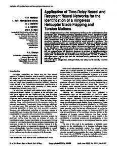
Fig. 1. Variations of the Unet based recurrent encoder-decoder networks for time-varying dense prediction. The second figure from left shows the CLSTM/CGRU bottleneck module configuration, where N denotes the number of channels, W and H are the spatial sizes of feature maps. The third figure from left shows the original Unet architecture. Our models were illustrated from fourth left to right most: Unet+CLSTM/CGRU-1, Unet+CLSTM/CGRU-3 and Unet+CLSTM/CGRU5. These networks were built by replacing convolution layers with 1, 3 and 5 CLSTM/CGRU bottleneck modules, respectively. Note that the line with bidirectional arrows in the rectangular box represents bidirectional CLSTM/CGRU. All convolution layers in these architectures use 3x3 kernels except for the output layer.
CLSTM can be formulated as: it ft ot
= = =
σ(Wi ∗ xt + Ui ∗ ht−1 ), σ(Wf ∗ xt + Uf ∗ ht−1 ), σ(Wo ∗ xt + Uo ∗ ht−1 ),
where it , ft , and ot are the input, forget, and output gates, respectively, σ is the sigmoidal activation function. Based on these gates, the recurrent function is defined as gt ct ht
= = =
tanh(Wg ∗ xt + Ug ∗ ht−1 ), ft ct−1 + it gt , ot tanh(ct ),
where ∗ denotes convolution and denotes element-wise multiplication. C. Convolutional GRU Similar to CLSTM, we improve the fully connected GRU gates to the convolutional gates as follows: = σ(Wz ∗ xt + Uz ∗ ht−1 ), = σ(Wr ∗ xt + Ur ∗ ht−1 ),
zt rt
where zt and rt are gates that control information flow between input, hidden unit and outputs, σ denotes the sigmoidal function. Based on these gates, the recurrent function is defined as: h˜t ht
= tanh(Wh xt + Uh (rt ht−1 )), = (1 − zt ) ∗ ht−1 + zt ∗ h˜t .
D. Deconvolutional LSTM and GRU The deconvolution layers in FCN were mainly used to enlarge the spatial resolution of feature maps for in dense prediction tasks [17]. We propose to integrate deconvolution operations into LSTM and GRU for the purpose of recovering spatial resolution while processing sequence in parallel. Formally, deconvolutional LSTM can be defined as: it ft ot gt ct ht
= = = = = =
σ(Wi ∗0 xt + Ui ∗ ht−1 ), σ(Wf ∗0 xt + Uf ∗ ht−1 ), σ(Wo ∗0 xt + Uo ∗ ht−1 ), tanh(Wg ∗0 xt + Ug ∗ ht−1 ), ft ct−1 + it gt , ot tanh(ct ),
where ∗0 denotes deconvolution, ∗ denotes convolution, and denotes element-wise multiplication. Similarly, deconvolutional GRU can be defined as: zt rt h˜t ht
= σ(Wz ∗0 xt + Uz ∗ ht−1 ), = σ(Wr ∗0 xt + Ur ∗ ht−1 ), = tanh(Wh ∗0 xt + Uh (rt ht−1 )), = (1 − zt ) ∗ ht−1 + zt ∗ h˜t .
E. The Proposed Bottleneck Module Unlike models that train FCN and CRNN separably [15], we aim at incorporating CRNN into FCN to build a single deep model that can be trained in an end-to-end fashion for time-varying dense prediction problems. CRNNs have multiple gates (e.g., 8 for CLSTM and 6 for CGRU), each performing convolution over input and hidden feature maps. Because the training of a recurrent layer is usually much more computationally intensive than training a convolution layer of the same size, directly adding recurrent convolutional layer to process all feature maps at the site of insertion leads to prohibitive computational and memory requirements. Specifically, CLSTM and CGRU layers resulted in 8 and 6, respectively, times increase in computation time and 3 times increase in memory usage. Given such excessive resource requirements, we propose to incorporate bottleneck modules into the recurrent convolutional layers [18]. Specifically, we stack a 1x1 convolution layer before the convolutional recurrent layers to reduce the number of feature maps. We also add a 1x1 convolution layer following the convolutional recurrent layer to restore the number of feature maps. The intermediate CRNN layer works as a bottleneck module that has much less resource requirements (Figure 1). This design effectively alleviates the computational resource requirements by reducing the number of trainable parameters, directly enabling the construction of a deep recurrent encoderdecoder network that has multiple recurrent layers. Our experimental results show that such networks are able to capture fine spatial structure and temporal contexts. F. Network Architectures In this work, we developed two architectures that combine FCN with CRNN. One uses a newly developed convolutional model, known as the “DenseNet”, as the FCN base model. DenseNet is an encoder-decoder network architecture that is very efficient and effective for general dense prediction problems [19], but does not have any recurrent connections.
A
Input 3x3 (32) Stride 2 3x3 (64)
1x7(64)
1x1 (128)
7x1 (64)
1x7 (128)
InceptionResidual A
1x1 (32) 3x3 (32)
1x1 (32) 3x3 (48)
1x1 (256) 1x1 (192)
1x7 (256)
3x3 (192) Stride 2
7x1 (320) 3x3 (320) Stride 2
3x3 (64)
InceptionResidual B
concat
1x1 (32)
+ 1x1 (192)
3x3(Maxpool) Stride 2
1x1 (256)
3x3 (32) Stride 2
concat
1x1 (192)
Reduction B
1x3 (224) 3x1 (256)
3x3 (256) 3x3 (384) Stride 2
Reduction A
1x1 (2048)
+
DLSTM (DGRU) 8X
3x3 (32) Stride 2
DLSTM (DGRU) 4X
+
3x3 (Maxpool) Stride 2 concat
1x1 (32)
Stem
1x1 (896)
concat 1x1 (96) Stride 2
1x1 (128) 7x1 (128)
3x3 (96)
1x1 (96)
DLSTM (DGRU) 2X
1x1 (64)
InceptionResidual C
DLSTM (DGRU) 16X
1x1 (64)
B
Input
concat
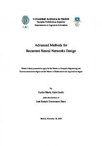
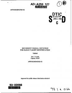
Fig. 2. The architecture of DenseNet+DLSTM/DGRU, a recurrent encoderdecoder network consisting of DenseNet and deconvolutional RNN (DLSTM/DGRU). Right: A concise view of the architecture that consists of building blocks of DenseNet and deconvolutional RNN layers. The building blocks of DenseNet include Stem, Inception-Residual A, Reduction A, InceptionResidual B, Reduction B and Inception-Residual C. Four output feature maps encoded by the DenseNet blocks with decreasing spatial resolutions are connected to DLSTM or DGRU layers to carry out two functions simultaneously; those are decoding feature maps to dense time-varying output by recovering spatial resolution and incorporating sequential context information. Left: detailed configuration of each building blocks of DenseNet. Note that the same block color indicate the same block between left figures and right figures and arrows denotes the output feature maps to DLSTM/DGRU.
need to employ the bottleneck architecture in DGRU/DCLSM layers. The encoding path of DenseNet consists of a set of carefully designed inception and residual modules for learning sophisticated feature representation, so no CRNN layer are inserted there to avoid hampering the network performance. For Unet, the hybrid model is built by replacing convolution layers at top feature hierarchies with CRNN layers. The CRNNs here also use LSTM or GRU units, so the corresponding hybrid models are termed Unet+CLSTM and Unet+CGRU, respectively. Because the CRNNs in Unet+ CLSTM/CGRU are applied on convolution layers with a lot of feature maps, bottleneck CRNN modules are used to reduce the computational cost, as described in section III-E. Additionally, to better evaluate the influence of CRNN layers on Unet, we tested 3 variants of either Unet+CLSTM or Unet+CGRU with increasing numbers of CRNN layers in the architecture (Figure 1). Altogether, the new models can be trained end-to-end. Either network takes time-varying dense input and produce dense prediction with spatiotemporal structures preserved. They inherited the power of FCN base models to deal with the multi-scale data (adaptive to large variance of the size of objects in the image), while being able to track the frame-toframe changes across the temporal dimension. IV.
DenseNet consists of a bottom-up path, which incorporates residual and inception modules for building hierarchical feature representation, and a top-down path, which uses deconvolution operations at various feature abstraction levels for decoding to produce dense predictions. The other architecture uses Unet as the base FCN model. Unet [20] is commonly used in bio-medical image segmentation. Its main idea is to combine the high-level (but low spatial resolution) and low-level (but high spatial resolution) features produced in the encoding path to gradually recover the segmentation resolution in the decoding path. Its encoding and decoding paths are symmetrical in multi-level feature combination, and it was not designed for time-varying dense prediction either. In this study, the original DenseNet and Unet were both used as baselines, whose performance will be compared in the context of the newly developed time-varying dense prediction models. The basic idea of combining FCN with CRNN is to insert CRNN layers into FCN architecture such that FCN layers are responsible for extracting hierarchical non-linear representations in spatial space, and CRNN layers are primarily for propagating the history of hierarchical temporal context features to sequential neighbors. The network as a whole would encode time-varying dense data in the input and decode it as dense prediction in the output. Specifically, for DenseNet, deconvolutional layers in the top-down path are replaced by deconvolutional RNN layers to build recurrent encoder-decoder dense prediction networks (Figure 2). The units in deconvolutional RNN layers are in the form of LSTM or GRU, the corresponding hybrid models are thus termed DenseNet+DLSTM and DenseNet+DGRU, respectively. Because the decoding path in DenseNet outputs only 2 feature maps at each feature scale, as a result, we do not
E XPERIMENTAL S TUDIES
To evaluate the two types of recurrent encoder-decoder networks for time-varying dense prediction, we applied them to neurite boundary prediction problems in 3D brain electron microscopy (EM) image dataset. Here, we considered the slice to slice correlation to be time-varying contextual information and each slice to be the frame of sequence. The mapping from raw image stack to the neurite boundary stack is a typical encoder-decoder dense prediction problem. As shown in Figure 1, for the hybrid network of Unet with CRNN, we evaluated 3 variants of this type of network with different layers of CLSTM/CGRU bottleneck modules (1, 3 and 5) added to Unet. For the combination of DenseNet and deconvolutional LSTM/GRU layers, there is only one variant. A. SNEMI3D Dataset The SNEMI3D challenge data [21] contains a stack of 100 1024 × 1024 slices. The stack is generated by serial section scanning electron microscopy (ssSEM) scanning of tissue sections along the Z-dimension. The stack is anisotropic in that it has high-resolution in the X-Y plane and low resolution along the Z-dimension. The image resolution is 6 × 6 × 30 nm/voxel that covers a micro-cube of approximately 6 × 6 × 3 microns. The dataset provides instance-based labels for neurite segmentation, which labels each voxel with the index of the neurite to which it belongs. A common approach for this segmentation task is to first discriminate the boundaries from neuron bodies by predicting boundary probability maps and then apply post-processing methods for generating instance level segmentation. We first transformed the neurite instance segmentation label into boundary label. The transformation was done by detecting the edges of instances and then marking pixels within distance of 3 pixels to the edges in either dimension as boundary. Because our goal is to assess the effectiveness of our approach in building models for time-varying
TABLE I.
C OMPARISON OF PERFORMANCE BETWEEN THE PROPOSED ENCODER - DECODER NETWORKS WITH BASELINE MODELS . I N THE PROPOSED MODELS , THE FCN COMPONENT COULD USE DIFFERENT ARCHITECTURES , SUCH AS THE U NET AND D ENSE N ET. S IMILARLY, THE RNN COMPONENT COULD USE CONVOLUTIONAL LSTM (CLSTM) OR GRU (CGRU), OR THEIR DECONVOLUTIONAL VARIANTS (DLSTM OR DGRU). T HE NUMBERS IN THE NAMES DENOTE THE NUMBER OF BOTTLENECK MODULES USED IN THE CORRESPONDING MODELS . FCN
Models RNN
CLSTM Unet CGRU
DenseNet
DLSTM DGRU
Model name Unet (baseline) Unet+CLSTM1 Unet+CLSTM3 Unet+CLSTM5 Unet+CGRU1 Unet+CGRU3 Unet+CGRU5 DenseNet (baseline) DenseNet+DLSTM DenseNet+DGRU
Accuracy 0.9087 0.9230 0.9241 0.9263 0.9104 0.9203 0.9106 0.9123 0.9253 0.9273
Measures AUC Rand error 0.9592 0.0623 0.9717 0.0540 0.9719 0.0528 0.9721 0.0498 0.9691 0.0592 0.9707 0.0556 0.9643 0.0610 0.9612 0.0601 0.9724 0.0465 0.9737 0.0482
dense prediction problems, it is appropriate to evaluate the performance of boundary probability map prediction instead of neurite instance segmentation. The evaluation was done on boundary probability maps directly since the segmentation results can be biased significantly by the post-processing methods, which is not related to time-varying dense prediction.
S2
S9
S14
Raw image
GT
Unet
Unet + CLSTM1
Unet + CLSTM5
DenseNet + DLSTM
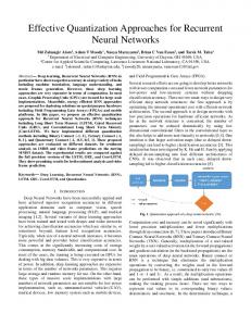
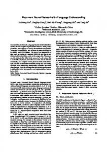
Fig. 3. Examples of dense prediction results. S2, S9, S14 are images at slice sequence of 2, 9, 14, respectively. The ground truth (GT), and predictions of networks by Unet, Unet+CLSTM1, Unet+CLSTM5 and DenseNet+DLSTM are shown. Each configuration of network architecture is depicted in Table I.
Three measures were used for evaluation. In addition to accuracy and area under the ROC curve (AUC) metrics, we also employed the adapted rand error metric, defined as: 1 the maximal F-score of the rand index, to assess the result. Details on adapted rand error were described in [22], [23].
rate of 0.001 with polynomial decay and a momentum of 0.9. The weights were initialized using Gaussian with STD of 0.01. Minimizing binary cross-entropy loss was chosen as our training objective. Upon inference, networks were given the entire 20 × 1024 × 1024 testing stack to produce boundary probability maps, which were then evaluated by three measures. We implemented network models using Keras with backend of Theano on CuDNNv5. The training took about 2 days for each networks on Tesla G40 GPU and the inference took about 2 minutes for each model. Our code is publicly available1 .
B. Experimental Setup
C. Experimental Results
We used the first 20 image slices of SNEMI3D data stack as test data and the remaining 80 image slices as training data. In building the hybrid FCN-CRNN networks for time-varying dense prediction, we considered two property of CRNN. The first is that, CRNN takes current input and feature representation of previous inputs captured in hidden units, and outputs feature maps that retain the same spatial structure as that of convolutional layers. The second is that, CRNN layer have more trainable convolutional kernels and additional hidden units compared to general convolutional layer.
The experimental results are given in table I. The results include the performance of hybrid networks that combine Unet with CRNN, with 3 variants of different layers of CLSTM/CGRU bottleneck modules (1, 3, and 5). The Table only contains the performance of models that combine DenseNet and deconvolutional LSTM/GRU layers.
Given the above facts, we built hybrid FCN-CRNN dense prediction networks by replacing part of the convolutional or deconvolutional layers with CRNN bottleneck modules, instead of adding additional CRNN layers to FCN. Such an approach allows the hybrid network to remain approximately the same number of trainable parameters, and carries out convolutional operations similar to those replaced convolutional layers while adding the capability of processing temporal context. To evaluate our newly proposed methods for building recurrent dense prediction networks against prior methods, we employed both the original Unet and DenseNet as baselines and compared them with the Unet based CLSTM/CGRU and DenseNet based DLSTM/DGRU. We trained each model for 20000 iterations with a minibatch of 3 of 7 × 256 × 256 3D patches that were randomly sampled from the training stack, where 7 indicating the number of sequential slices in the Z-direction. Networks were optimized with stochastic gradient descent at base learning
We can observe that Unet+CLSTM5, a dense prediction network built upon Unet and 5 CLSTM bottleneck modules, yielded better results in all three metrics as compared to 2 other variants of Unet+CLSTM models. Comparing to the baseline Unet model, all variants of Unet+CLSTM models achieved better results in 3 measurement metrics. We can also observe that the model achieved better performance as more CLSTM bottleneck modules were being used. This, however, was not the case in the Unet+CGRU models. Instead, Unet+CGRU3, which employed 3 CGRU bottleneck modules, obtained slightly better performance than both Unet+CGRU1 and Unet+CGRU5 in all 3 metrics. Among all variants of Unet+CRNN, Unet+CLSTM5 achieved the highest performance in our experiments. In the case of DenseNet+CRNN architecture, experimental results showed that models with LSTM or GRU recurrent layers yielded roughly similar results. DenseNet+DGRU, which employed deconvolutional GRU layers, achieved slightly better performance in accuracy and AUC but slightly worse performance in rand error. Both variants were better in all three metrics compared to the baseline DenseNet. Comparison between the two types of models showed that the architecture that 1 https://github.com/divelab/crnn
combines DenseNet with deconvolutional RNN outperformed Unet based models in our experiments. Their performance was better for almost every metric.
[3]
[4]
V.
C ONCLUSIONS AND D ISCUSSIONS
In this work, we approached the time-varying dense prediction problems by considering it as learning a mapping function from raw image sequence to output label sequence of the same size. Accordingly, we built recurrent encoder-decoder networks to learn such mapping functions. The proposed network encodes the inputs as hierarchical feature representations and decodes them similarly from multiple hierarchies in the output space. The idea behind the networks is to exploit the power of both FCN and CRNN to jointly learn spatiotemporal feature representations. We used Unet and DenseNet as baselines to build the proposed network architecture, but the proposed bottleneck modules can be integrated with any generic deep models. The CRNN and DRNN were modified from conventional RNN, in which fully connected operations were replaced by convolutional and deconvolutional kernels, respectively. Such changes allow CRNN/DRNN to preserve spatial structures while processing temporal context information. To assess the effects of using different numbers of CRNN layers, we proposed a novel CRNN bottleneck module to allow more CRNN layers to be used while alleviating the computational and memory requirements. The results of our experiments showed that embedding CRNN layers into FCN clearly improves the network performance, measured by three metrics. This is true for both hybrid network models proposed in this work. We also demonstrated that more CRNN layers would lead to better performance, particularly with CLSTM bottleneck modules. When comparing two hybrid models, our DenseNet-based architecture combined with DRNN yielded better overall performance than that of Unet based architecture.
[5] [6] [7]
[8] [9]
[10]
[11]
[12]
[13]
[14]
[15]
This work focused on segmenting 3D volumetric biomedical imaging data. The proposed methods are generic and can be applied to solve general time-varying dense prediction problems. We will extend our approach to other time-varying dense prediction tasks in the future, such as dense action and physical motion prediction. Such extension will allow us to fully explore the limits of our network models and adapt them to wider range of applications.
[18]
ACKNOWLEDGMENT
[19]
This work was supported in part by National Science Foundation grants DBI-1641223, IIS-1615035, IIS-1565596, IIS-1615597, and Office of Naval Research grant N00014-141-0631.
[16]
[17]
[20]
[21]
R EFERENCES [1]
[2]
Y. LeCun, L. Bottou, Y. Bengio, and P. Haffner, “Gradient-based learning applied to document recognition,” Proceedings of the IEEE, vol. 86, no. 11, pp. 2278–2324, November 1998. A. Krizhevsky, I. Sutskever, and G. Hinton, “Imagenet classification with deep convolutional neural networks,” in Advances in Neural Information Processing Systems 25, P. Bartlett, F. Pereira, C. Burges, L. Bottou, and K. Weinberger, Eds., 2012, pp. 1106–1114.
[22]
[23]
C. Szegedy, W. Liu, Y. Jia, P. Sermanet, S. Reed, D. Anguelov, D. Erhan, V. Vanhoucke, and A. Rabinovich, “Going deeper with convolutions,” in Proceedings of the IEEE Conference on Computer Vision and Pattern Recognition, 2015, pp. 1–9. C. Szegedy, S. Ioffe, and V. Vanhoucke, “Inception-v4, inception-resnet and the impact of residual connections on learning,” arXiv preprint arXiv:1602.07261, 2016. Y. LeCun, Y. Bengio, and G. Hinton, “Deep learning,” Nature, vol. 521, no. 7553, pp. 436–444, 2015. S. Hochreiter and J. Schmidhuber, “Long short-term memory,” Neural Computation, vol. 9, no. 8, pp. 1735–1780, 1997. J. Long, E. Shelhamer, and T. Darrell, “Fully convolutional networks for semantic segmentation,” in Proceedings of the IEEE Conference on Computer Vision and Pattern Recognition, 2015, pp. 3431–3440. P. O. Pinheiro, T.-Y. Lin, R. Collobert, and P. Doll´ar, “Learning to refine object segments,” arXiv preprint arXiv:1603.08695, 2016. S. Zagoruyko, A. Lerer, T.-Y. Lin, P. O. Pinheiro, S. Gross, S. Chintala, and P. Doll´ar, “A multipath network for object detection,” arXiv preprint arXiv:1604.02135, 2016. M. Liang, X. Hu, and B. Zhang, “Convolutional neural networks with intra-layer recurrent connections for scene labeling,” in Advances in Neural Information Processing Systems, 2015, pp. 937–945. J. Donahue, L. Anne Hendricks, S. Guadarrama, M. Rohrbach, S. Venugopalan, K. Saenko, and T. Darrell, “Long-term recurrent convolutional networks for visual recognition and description,” in Proceedings of the IEEE Conference on Computer Vision and Pattern Recognition, 2015, pp. 2625–2634. M. F. Stollenga, W. Byeon, M. Liwicki, and J. Schmidhuber, “Parallel multi-dimensional LSTM, with application to fast biomedical volumetric image segmentation,” in Advances in Neural Information Processing Systems, 2015, pp. 2980–2988. L. Yao, A. Torabi, K. Cho, N. Ballas, C. Pal, H. Larochelle, and A. Courville, “Describing videos by exploiting temporal structure,” in Proceedings of the IEEE international conference on computer vision, 2015, pp. 4507–4515. N. Srivastava, E. Mansimov, and R. Salakhudinov, “Unsupervised learning of video representations using LSTMs,” in Proceedings of the 32nd International Conference on Machine Learning, 2015, pp. 843– 852. X. Shi, Z. Chen, H. Wang, D.-Y. Yeung, W.-k. Wong, and W.-c. WOO, “Convolutional LSTM network: A machine learning approach for precipitation nowcasting,” in Advances in Neural Information Processing Systems, 2015, pp. 802–810. J. Chen, L. Yang, Y. Zhang, M. Alber, and D. Z. Chen, “Combining fully convolutional and recurrent neural networks for 3d biomedical image segmentation,” in Advances in Neural Information Processing Systems, 2016, pp. 3036–3044. H. Noh, S. Hong, and B. Han, “Learning deconvolution network for semantic segmentation,” in Proceedings of the IEEE International Conference on Computer Vision, 2015, pp. 1520–1528. K. He, X. Zhang, S. Ren, and J. Sun, “Deep residual learning for image recognition,” in Proceedings of the IEEE Conference on Computer Vision and Pattern Recognition, 2016. A. Fakhry, T. Zeng, and S. Ji, “Residual deconvolutional networks for brain electron microscopy image segmentation,” IEEE Transactions on Medical Imaging, 2016. O. Ronneberger, P. Fischer, and T. Brox, “U-net: Convolutional networks for biomedical image segmentation,” in International Conference on Medical Image Computing and Computer-Assisted Intervention. Springer, 2015, pp. 234–241. N. Kasthuri, K. J. Hayworth, D. R. Berger, R. L. Schalek, J. A. Conchello, S. Knowles-Barley, D. Lee, A. V´azquez-Reina, V. Kaynig, T. R. Jones et al., “Saturated reconstruction of a volume of neocortex,” Cell, vol. 162, no. 3, pp. 648–661, 2015. T. Liu, C. Jones, M. Seyedhosseini, and T. Tasdizen, “A modular hierarchical approach to 3d electron microscopy image segmentation,” Journal of neuroscience methods, vol. 226, pp. 88–102, 2014. A. Fakhry, H. Peng, and S. Ji, “Deep models for brain EM image segmentation: novel insights and improved performance,” Bioinformatics, vol. 32, pp. 2352–2358, 2016.