But I don’t want to go to bed now!
But I don't
to go to bed now!
want
. An HTML document.
The main document has three components: the element, with its contents; the
element, with its contents; and the blank space in between. The
element, in turn, has three components: the untagged text before the element; the element, with its contents; and the untagged text after the element. The element has one component, which is the untagged text What Junior Said Next. In Chapter 8, we’ll see how to build parsers for languages like HTML. In the meantime, we’ll look at a semi-standard module, HTML::TreeBuilder, which converts an HTML document into a tree structure. Let’s suppose that the HTML data is already in a variable, say $html. The following code uses HTML::TreeBuilder to transform the text into an explicit tree structure: use HTML::TreeBuilder; my $tree = HTML::TreeBuilder->new; $tree->ignore_ignorable_whitespace(0); $tree->parse($html); $tree->eof();
The ignore_ignorable_whitespace() method tells HTML::TreeBuilder that it’s not allowed to discard certain whitespace, such as the newlines after the element, that are normally ignorable. Now $tree represents the tree structure. It’s a tree of hashes; each hash is a node in the tree and represents one element. Each hash has a _tag key whose value is its tag name, and a _content key whose value is a list of the element’s contents, in order; each item in the _content list is either a string, representing tagless text, or another hash, representing another element. If the tag also has attribute–value pairs, they’re stored in the hash directly, with attributes as hash keys and the corresponding values as hash values.
27
28
Recursion and Callbacks
So for example, the tree node that corresponds to the element in the example looks like this: { _tag => "font", _content => [ "want" ], color => "red", size => 3, }
The tree node that corresponds to the and looks like this:
element contains the
node,
{ _tag => "p", _content => [ "But I don't ", { _tag => "font", _content => [ "want" ], color => "red", size => 3, }, " to go to bed now!", ], }
It’s not hard to build a function that walks one of these HTML trees and “untags” all the text, stripping out the tags. For each item in a _content list, we can recognize it as an element with the ref() function, which will yield true for elements (which are hash references) and false for plain strings: CO DE LIB R A RY
sub untag_html {
untag-html
my ($html) = @_; return $html unless ref $html;
# It’s a plain string
my $text = ''; for my $item (@{$html->{_content}}) { $text .= untag_html($item); }
return $text; }
The function checks to see if the HTML item passed in is a plain string, and if so the function returns it immediately. If it’s not a plain string, the function
.
29
assumes that it is a tree node, as described above, and iterates over its content, recursively converting each item to plain text, accumulating the resulting strings, and returning the result. For our example, this is: What Junior Said Next But I don't want to go to bed now!
Sean Burke, the author of HTML::TreeBuilder, tells me that accessing the internals of the HTML::TreeBuilder objects this way is naughty, because he might change them in the future. Robust programs should use the accessor methods that the module provides. In these examples, we will continue to access the internals directly. We can learn from dir_walk() and make this function more useful by separating it into two parts: the part that processes an HTML tree, and the part that deals with the specific task of assembling plain text: sub walk_html {
COD E L IB RARY
my ($html, $textfunc, $elementfunc) = @_; return $textfunc->($html) unless ref $html; # It’s a plain string
my @results; for my $item (@{$html->{_content}}) { push @results, walk_html($item, $textfunc, $elementfunc); } return $elementfunc->($html, @results); }
This function has exactly the same structure as dir_walk(). It gets two auxiliary functions as arguments: a $textfunc that computes some value of interest for a plain text string, and an $elementfunc that computes the corresponding value for an element, given the element and the values for the items in its content. $textfunc is analogous to the $filefunc from dir_walk(), and $elementfunc is analogous to the $dirfunc. Now we can write our untagger like this: walk_html($tree, sub { $_[0] }, sub { shift; join '', @_ });
The $textfunc argument is a function that returns its argument unchanged. The $elementfunc argument is a function that throws away the element itself, then concatenates the texts that were computed for its contents, and returns the concatenation. The output is identical to that of untag_html().
walk-html
30
Recursion and Callbacks
Suppose we want a document summarizer that prints out the text that is inside of tags and throws away everything else: sub print_if_h1tag { my $element = shift; my $text = join '', @_; print $text if $element->{_tag} eq 'h1'; return $text; } walk_html($tree, sub { $_[0] }, \&print_if_h1tag);
This is essentially the same as untag_html(), except that when the element function sees that it is processing an element, it prints out the untagged text. If we want the function to return the header text instead of printing it out, we have to get a little trickier. Consider an example like this: Junior Is a naughty boy.
We would like to throw away the text Is a naughty boy, so that it doesn’t appear in the result. But to walk_html(), it is just another plain text item, which looks exactly the same as Junior, which we don’t want to throw away. It might seem that we should simply throw away everything that appears inside a non-header tag, but that doesn’t work: The story of Junior
We mustn’t throw away Junior here, just because he’s inside a tag, because that tag is itself inside an tag, and we want to keep it. We could solve this problem by passing information about the current tag context from each invocation of walk_html() to the next, but it turns out to be simpler to pass information back the other way. Each text in the file is either a “keeper,” because we know it’s inside an element, or a “maybe,” because we don’t. Whenever we process an element, we’ll promote all the “maybes” that it contains to “keepers.” At the end, we’ll print the keepers and throw away the maybes: CO DE LIB R A RY
@tagged_texts = walk_html($tree, sub { ['MAYBE', $_[0]] },
extract-headers
\&promote_if_h1tag); sub promote_if_h1tag {
. my $element = shift; if ($element->{_tag} eq 'h1') { return ['KEEPER', join '', map {$_->[1]} @_]; } else { return @_; } }
The return value from walk_html() will be a list of labeled text items. Each text item is an anonymous array whose first element is either MAYBE or KEEPER, and whose second item is a string. The plain text function simply labels its argument as a MAYBE. For the string Junior, it returns the labeled item ['MAYBE', 'Junior']; for the string Is a naughty boy., it returns ['MAYBE', 'Is a naughty boy.']. The element function is more interesting. It gets an element and a list of labeled text items. If the element represents an tag, the function extracts all the texts from its other arguments, joins them together, and labels the result as a KEEPER. If the element is some other kind, the function returns its tagged texts unchanged. These texts will be inserted into the list of labeled texts that are passed to the element function call for the element that is one level up; compare this with the final example of dir_walk() in Section 1.5, which returned a list of filenames in a similar way. Since the final return value from walk_html() is a list of labeled texts, we need to filter them and throw away the ones that are still marked MAYBE. This final pass is unavoidable. Since the function treats an untagged text item differently at the top level than it does when it is embedded inside an tag, there must be some part of the process that understands when something is at the top level. walk_html() can’t do that because it does the same thing at every level. So we must build one final function to handle the top-level processing: sub extract_headers { my $tree = shift; my @tagged_texts = walk_html($tree, sub { ['MAYBE', $_[0]] }, \&promote_if_h1tag); my @keepers = grep { $_->[0] eq 'KEEPER'} @tagged_texts; my @keeper_text = map { $_->[1] } @keepers; my $header_text = join '', @keeper_text; return $header_text; }
Or we could write it more compactly: sub extract_headers { my $tree = shift;
31
32
Recursion and Callbacks my @tagged_texts = walk_html($tree, sub { ['MAYBE', $_[0]] }, \&promote_if_h1tag); join '', map { $_->[1] } grep { $_->[0] eq 'KEEPER'} @tagged_texts; }
1.7.1 More Flexible Selection We just saw how to extract all the -tagged text in an HTML document. The essential procedure was promote_if_h1tag(). But we might come back next time and want to extract a more detailed summary, which included all the text from , , , and any other tags present. To get this, we’d need to make a small change to promote_if_h1tag() and turn it into a new function: sub promote_if_h1tag { my $element = shift; if ($element->{_tag} =˜ /∧ h\d+$/) { return ['KEEPER', join '', map {$_->[1]} @_]; } else { return @_; } }
But if promote_if_h1tag is more generally useful than we first realized, it will be a good idea to factor out the generally useful part. We can do that by parametrizing the part that varies: CO DE LIB R A RY
sub promote_if {
promote-if
my $is_interesting = shift; my $element = shift; if ($is_interesting->($element->{_tag}) { return ['KEEPER', join '', map {$_->[1]} @_]; } else { return @_; } }
Now instead of writing a special function, promote_if_h1tag(), we can express the same behavior as a special case of promote_if(). Instead of the following: my @tagged_texts = walk_html($tree, sub { ['maybe', $_[0]] }, \&promote_if_h1tag);
.
we can use this: my @tagged_texts = walk_html($tree, sub { ['maybe', $_[0]] }, sub { promote_if( sub { $_[0] eq 'h1'}, $_[0]) });
We’ll see a tidier way to do this in Chapter 7.
1.8 Sometimes a problem appears to be naturally recursive, and then the recursive solution is grossly inefficient. A very simple example arises when you want to compute Fibonacci numbers. This is a rather unrealistic example, but it has the benefit of being very simple. We’ll see a more practical example of the same thing in Section 3.7.
1.8.1 Fibonacci Numbers Fibonacci numbers are named for Leonardo of Pisa, whose nickname was Fibonacci, who discussed them in the 13th century in connection with a mathematical problem about rabbits. Initially, you have one pair of baby rabbits. Baby rabbits grow to adults in one month, and the following month they produce a new pair of baby rabbits, making two pairs: Month 1 2 3
Pairs of baby rabbits 1 0 1
Pairs of adult rabbits 0 1 1
Total pairs 1 1 2
The following month, the baby rabbits grow up and the adults produce a new pair of babies: 4
1
2
3
The month after that, the babies grow up, and the two pairs of adults each produce a new pair of babies: 5
2
3
5
33
34
Recursion and Callbacks
Assuming no rabbits die, and rabbit production continues, how many pairs of rabbits are there in each month? Let A(n) be the number of pairs of adults alive in month n and B(n) be the number of pairs of babies alive in month n. The total number of pairs of rabbits alive in month n, which we’ll call T(n), is therefore A(n) + B(n): T (n) = A(n) + B(n) It’s not hard to see that the number of baby rabbits in one month is equal to the number of adult rabbits the previous month, because each pair of adults gives birth to one pair of babies. In symbols, this is B(n) = A(n − 1). Substituting into our formula, we have: T (n) = A(n) + A(n − 1) Each month the number of adult rabbits is equal to the total number of rabbits from the previous month, because the babies from the previous month grow up and the adults from the previous month are still alive. In symbols, this is A(n) = T(n − 1). Substituting into the previous equation, we get: T (n) = T (n − 1) + T (n − 2) So the total number of rabbits in month n is the sum of the number of rabbits in months n − 1 and n − 2. Armed with this formula, we can write down the function to compute the Fibonacci numbers: CO DE LIB R A RY fib
# Compute the number of pairs of rabbits alive in month n sub fib { my ($month) = @_; if ($month < 2) { 1 } else { fib($month-1) + fib($month-2); } }
.
This is perfectly straightforward, but it has a problem: except for small arguments, it takes forever.4 If you ask for fib(25), for example, it needs to make recursive calls to compute fib(24) and fib(23). But the call to fib(24) also makes a recursive call to fib(23), as well as another to compute fib(22). Both calls to fib(23) will also call fib(22), for a total of three times. It turns out that fib(21) is computed 5 times, fib(20) is computed 8 times, and fib(19) is computed 13 times. All this computing and recomputing has a heavy price. On my small computer, it takes about four seconds to compute fib(25); it makes 242,785 recursive calls while doing so. It takes about 6.5 seconds to compute fib(26), and makes 392,835 recursive calls, and about 10.5 seconds to make the 635,621 recursive calls for fib(27). It takes as long to compute fib(27) as to compute fib(25) and fib(26) put together, and so the running time of the function increases rapidly, more than doubling every time the argument increases by 2.5 The running time blows up really fast, and it’s all caused by our repeated computation of things that we already computed. Recursive functions occasionally have this problem, but there’s an easy solution for it, which we’ll see in Chapter 3.
1.8.2 Partitioning Fibonacci numbers are rather abstruse, and it’s hard to find simple realistic examples of programs that need to compute them. Here’s a somewhat more realistic example. We have some valuable items, which we’ll call “treasures,” and we want to divide them evenly between two people. We know the value of each item, and we would like to ensure that both people get collections of items whose total value is the same. Or, to recast the problem in a more mundane light: we know the weight of each of the various groceries you bought today, and since you’re going to carry them home with one bag in each hand, you want to distribute the weight evenly. To convince yourself that this can be a tricky problem, try dividing up a set of ten items that have these dollar values: $9,
4
5
$12,
$14,
$17,
$23,
$32,
$34,
$40,
$42,
and
$49
One of the technical reviewers objected that this was an exaggeration, and it is. But I estimate that calculating fib(100) by this method would take about 2,241,937 billion billion years, which is close enough. In fact, each increase of 2 in the argument increases the running time by a factor of about 2.62.
35
36
Recursion and Callbacks
Since the total value of the items is $272, each person will have to receive items totalling $136. Then try: $9,
$12,
$14,
$17,
$23,
$32,
$34,
$40,
$38,
and
$49
Here I replaced the $42 item with a $38 item, so each person will have to receive items totalling $134. This problem is called the partition problem. We’ll generalize the problem a little: instead of trying to divide a list of treasures into two equal parts, we’ll try to find some share of the treasures whose total value is a given target amount. Finding an even division of the treasures is the same as finding a share whose value is half of the total value of all the treasures; then the other share is the rest of the treasures, whose total value is the same. If there is no share of treasures that totals the target amount, our function will return undef: CO DE LIB R A RY
sub find_share {
find-share
my ($target, $treasures) = @_; return [] if $target == 0; return
if $target < 0 || @$treasures == 0;
We take care of some trivial cases first. If the target amount is exactly zero, then it’s easy to produce a list of treasures that total the target amount: the empty list is sure to have value zero, so we return that right away. If the target amount is less than zero, we can’t possibly hit it, because treasures are assumed to have positive value. In this case no solution can be found and the function can immediately return failure. If there are no treasures, we know we can’t make the target, since we already know the target is larger than zero; we fail immediately. Otherwise, the target amount is positive, and we will have to do some real work: my ($first, @rest) = @$treasures; my $solution = find_share($target-$first, \@rest); return [$first, @$solution] if $solution; return
find_share($target
, \@rest);
}
Here we copy the list of treasures, and then remove the first treasure from the list. This is because we’re going to consider the simpler problem of how to divide up the treasures without the first treasure. There are two possible divisions: either this first treasure is in the share we’re computing, or it isn’t. If it is, then we
.
have to find a subset of the rest of the treasures whose total value is $target $first. If it isn’t, then we have to find a subset of the rest of the treasures whose total value is $target. The rest of the code makes recursive calls to find_share to investigate these two cases. If the first one works out, the function returns a solution that includes the first treasure; if the second one works out, it returns a solution that omits the first treasure; if neither works out, it returns undef. Here’s a trace of a sample run. We’ll call find_share(5, [1, 2, 4, 8]): Share so far
Total so far 0
Target 5
Remaining treasures 1248
None of the trivial cases apply — the target is neither negative nor zero, and the remaining treasure list is not empty — so the function tries allocating the first item, 1, to the share; it then looks for some set of the remaining items that can be made to add up to 4: 1
1
4
248
The function will continue investigating this situation until it is forced to give up. The function then allocates the first remaining item, 2, toward the share of 4, and makes a recursive call to find some set of the last 2 elements that add up to 2: 12
3
2
48
Let’s call this “situation a.” The function will continue investigating this situation until it concludes that situation a is hopeless. It tries allocating the 4 to the share, but that overshoots the target total: 124
7
−2
8
so it backs up and tries continuing from situation a without allocating the 4 to the share: 12
3
2
8
The share is still wanting, so the function allocates the next item, 8, to the share, which obviously overshoots: 128
11
−6
Here we have $target < 0, so the function fails, and tries omitting 8 instead. This doesn’t work either, as it leaves the share short by 2 of the target, with no
37
38
Recursion and Callbacks
items left to allocate: Share so far 12
Total so far
Target
3
2
Remaining treasures
This is the if (@$treasures == 0) { return undef } case. The function has tried every possible way of making situation a work; they all failed. It concludes that allocating both 1 and 2 to the share doesn’t work, and backs up and tries omitting 2 instead: 1
1
4
48
0
8
It now tries allocating 4 to the share: 14
5
Now the function has $target == 0, so it returns success. The allocated treasures are 1 and 4, which add up to the target 5. The idea of ignoring the first treasure and looking for a solution among the remaining treasures, thus reducing the problem to a simpler case, is natural. A solution without recursion would probably end up duplicating the underlying machinery of the recursive solution, and simulating the behavior of the functioncall stack manually. Now solving the partition problem is easy; it’s a call to find_share(), which finds the first share, and then some extra work to compute the elements of the original array that are not included in the first share: CO DE LIB R A RY partition
sub partition { my $total = 0; my $share_2; for my $treasure (@_) { $total += $treasure; }
my $share_1 = find_share($total/2, [@_]); return unless defined $share_1;
First the function computes the total value of all the treasures. Then it asks find_share() to compute a subset of the original treasures whose total value is exactly half. If find_share() returns an undefined value, there was no equal division, so partition() returns failure immediately. Otherwise, it will set about
.
computing the list of treasures that are not in second share:
$share_1,
and this will be the
my %in_share_1; for my $treasure (@$share_1) { ++$in_share_1{$treasure}; } for my $treasure (@_) { if ($in_share_1{$treasure}) { --$in_share_1{$treasure}; } else { push @$share_2, $treasure; } }
The function uses a hash to count up the number of occurrences of each value in the first share, and then looks at the original list of treasures one at a time. If it saw that a treasure was in the first share, it checks it off; otherwise, it put the treasure into the list of treasures that make up share 2. return ($share_1, $share_2); }
When it’s done, it returns the two lists of treasures. There’s a lot of code here, but it mostly has to do with splitting up a list of numbers. The key line is the call to find_share(), which actually computes the solution; this is $share_1. The rest of the code is all about producing a list of treasures that aren’t in $share_1; this is $share_2. The find_share function, however, has a problem: it takes much too long to run, especially if there is no solution. It has essentially the same problem as fib did: it repeats the same work over and over. For example, suppose it is trying to find a division of 1 2 3 4 5 6 7 with target sum 14. It might be investigating shares that contain 1 and 3, and then look to see if it can make 5 6 7 hit the target sum of 10. It can’t, so it will look for other solutions. Later on, it might investigate shares that contain 4, and again look to see if it can make 5 6 7 hit the target sum of 10. This is a waste of time; find_share should remember that 5 6 7 cannot hit a target sum of 10 from the first time it investigated that. We will see in Chapter 3 how to fix this.
39