Any scalar products of the momenta in the numerator are reduced to powers. 1For a review of existing packages see Ref.[2]. 2This package can be used also in ...
Recursion relations for two-loop self-energy diagrams on shell.
arXiv:hep-ph/9905379v1 18 May 1999
J. Fleischer, M. Yu. Kalmykov, A. V. Kotikov Fakult¨ at f¨ ur Physik, Universit¨at Bielefeld, D-33615 Bielefeld 1, Germany Abstract A set of recurrence relations for on-shell two-loop self-energy diagrams with one mass is presented, which allows to reduce the diagrams with arbitrary indices (powers of scalar propagators) to a set of the master integrals. The SHELL2 package is used for the calculation of special types of diagrams. A method of calculation of higher order εexpansion of master integrals is demonstrated.
Nowadays e+ e− -experiments are sensitive to multiloop radiative corrections. The transverse part of renormalized gauge boson self-energies on mass shell enter a wide class of low energy observables like ∆ρ, ∆r, etc. Keeping in mind this physical application we elaborate a FORM [1] based package 1 [3] for analytical calculations of on-shell two-loop self-energy diagrams with one mass 2 . All possible diagrams of given type are shown on Fig.1. The diagrams implemented in the package SHELL2 [5] (ON3, ON2 in our notations) and those considered in detail in Ref.[6] (F00000, V0000, J001, J000) are not discussed here. In contrary to Ref.[7] we used only recurrence relations obtained from the integration by part method [6] without shifting the dimension of space-time. Here we apply the triangle rule for arbitrary masses and external momentum given in Ref.[8]. We are working in Euclidean space-time with dimension N = 4 − 2ε. The general prototype involves arbitrary integer powers of the scalar denominators cL = kL2 + m2L . For completeness we write below our notations: c1 = k12 +m21 , c2 = k22 +m22 , c3 = (k1 −p)2 +m23 , c4 = (k2 −p)2 +m44 , c5 = (k1 −k2 )2 +m25 . Their powers jL are called indices of the lines. The mass-shell condition for the external momentum now is p2 = −m2 . Any scalar products of the momenta in the numerator are reduced to powers 1 2
For a review of existing packages see Ref.[2]. This package can be used also in asymptotic expansion, see, e.g.[4].
1
of the scalar propagators (in case of V and J topologies the corresponding lines are added). Thus, the indices may sometimes become negative. The recurrence relations allow to reduce all lines with negative indices to zero and the positive indices to one or zero. F-topology. Let us consider the diagram of F-type:
m 22
m 21 k2
k1 2 5
m m
2 3
k1 -p
p2 =-m 2 k2 -p m24
The full set of recurrence relations valid for arbitrary p2 , m21 , m22 , m23 , m24 , m25 is the following: {135}
N − 2j1 − j3 − j5 +
� j1 2 j3 � 2 m3 + m21 − m2 − c1 2m1 + c1 c3
� j5 � 2 m5 + m21 − m22 + c2 − c1 = 0, c5 � j1 � 2 j3 m3 + m21 − m2 − c3 N − 2j3 − j1 − j5 + 2m23 + c3 c1 � � j5 + m25 + m23 − m24 + c4 − c3 = 0, c5 � j5 j1 � 2 N − 2j5 − j1 − j3 + 2m25 + m5 + m21 − m22 + c2 − c5 c5 c1 � � j3 m25 + m23 − m24 + c4 − c5 = 0, + c3 � j4 � 2 j2 m4 + m22 − m2 − c2 N − 2j2 − j4 − j5 + 2m22 + c2 c4 � � j5 m25 + m22 − m21 + c1 − c2 = 0, + c5 � j4 j2 � 2 N − 2j4 − j2 − j5 + 2m24 + m4 + m22 − m2 − c4 c4 c2 � j5 � 2 m5 + m24 − m23 + c3 − c4 = 0, + c5 � j5 j2 � 2 N − 2j5 − j2 − j4 + 2m25 + m5 + m22 − m21 + c1 − c5 c5 c2
+ {315}
{513}
{245}
{425}
{524}
2
+
� j4 � 2 m5 + m24 − m23 + c3 − c5 = 0, c4
where both sides of these relations are understood to be multiplied by R dN k1 dN k2 j1 j2 j3 j4 j5 . Due to the symmetry of the diagram it is sufficient to consider c1 c2 c3 c4 c5
|j |
in detail only the cases j1 < 0 (c1 1 in the numerator) and j5 < 0. To exclude the numerator in the first case, we apply the following relations. If j5 6= 1 we solve Eq.{245} with respect to the cj55 c1 term. If j2 6= 1 the cj22 c1 term of {524} is used. For j3 6= 1 the linear combination {245} + {135} is solved with respect to cj33 c1 . In case j2 = j3 = j5 = 1 we apply {315}, solved with respect to the free term (N − 3 − j1 ), to create a denominator for which the above given relations are applicable. The case j5 < 0 is considered in detail in Refs.[6, 7, 9]. In this manner F-type integrals with arbitrary indices are reduced to F-type integrals with only positive indices or Vtype integrals with arbitrary indices. For the former case the solution of recurrence relations is presented in Ref.[3]. Only eight diagrams F11111, F00111, F10101, F10110, F01100, F00101, F10100, F00001 with all indices equal to 1 form the F-type basis. V-topology. Let us consider the V-type topology: k 2-p m
2 2
m25 m
2 3
p2 =-m2 k2 m24
k1
The set of recurrence relations, valid for arbitrary mass and momenta, consist of relation {425} and the following ones: � j2 � 2 j4 m4 + m22 − m2 − c4 2m24 + c4 c2
{423}
N − 2j4 − j2 − j3 +
{530}
� j3 � 2 m3 + m24 − m25 + c5 − c4 = 0, c3 � j3 � 2 j5 m3 + m25 − m24 + c4 − c5 = 0, N − 2j5 − j3 + 2m25 + c5 c3 � j3 j5 � 2 N − 2j3 − j5 + 2m23 + m5 + m23 − m24 + c4 − c3 = 0, c3 c5
+
{350}
3
� j3 j5 j5 � 2 [NUM] − m4 − m22 + m2 + c2 − c4 = 0, + c3 c5 c5 � �� � j2 j4 j5 + + m24 − m22 + m2 + c2 − c4 c2 c4 c5 j2 j5 − [NUM] − 2m2 = 0, c5 c2 � � � j2 j4 j5 � 2 j2 m5 − m23 − m24 + c3 + c4 − c5 [NUM] + + + c2 c2 c4 c5 � j5 � c3 − m2 = 0, −2 c5
�
{A} {B}
{C}
�
where we introduce [NUM] ≡
(m24 − m22 + m2 + c2 − c4 ) (m25 − m23 − m24 + c3 + c4 − c5 ) , 2c6
c6 = c4 − m24 and the zero-index in the above relations denotes lines with zero mass and zero index. Let us discuss in detail the relations {A, B, C}. Due to the presence of a four-line vertex in this case, some scalar product arising in the recurrence relations cannot be expressed as linear combination of denominators. Nevertheless this scalar product can be presented as a nonlinear combination of a denominator and a ‘new’ massless propagator (see Ref.[10]). Let us consider the following distribution of momenta: c2 = (k2 + p)2 + m22 ; c3 = k12 + m23 ; c4 = k22 + m44 ; c5 = (k1 − k2 )2 + m25 . Then relation {B} reads 0≡
Z
∂ d k2 µ ∂k2 N
(
pµ cj22 cj44 cj55
)
→ 2m2
j2 j5 j2 j4 j5 − 2 k1 p − + + k2 p = 0. c2 c5 c2 c4 c5 �
�
The scalar product k2 p is rewritten in the following way: k2 p = c2 −c4 +m4 − m2 + m2 , whereas k1 p can be presented by means of the � projection � operator: µ pν 2) µ δ − , where A(q, r, p, ) = q k1 p = A(k1 , p, k2) + (k1 k2k)(pk r ν satisfies 2 µν p2 2 the property that odd power of A(q, r, p) drop out after integration. Due (m2 −m2 +m2 +c2 −c4 )(m25 −m23 −m24 +c3 +c4 −c5 ) , where to this property we have k1 p = 4 2 4c6 1 2 2 c6 = c4 − m4 . If m4 6= 0, the expression c4 c6 can be simplified by partial fraction decomposition. Numerator for V-topology. For j2 , j3 or j5 < 0 the initial diagram can be reduced to a two-loop tadpole-like integral by Eq.(2.10) in [11]. For j4 < 0 4
we apply the following relations. If j5 6= 1 we solve Eq.{350} with respect to the cj55 c4 term. If j3 6= 1 the cj33 c4 term of {530} is used. For j2 6= 1 the linear combination {425} + {350} is solved with respect to cj22 c4 . The case j2 = j3 = j5 = 1 requires additional consideration. We distinguish the following cases for on-shell integrals: 1. m23 = m25 = m2 , m22 = 0. j2 j5 c5 − c3 j5 2 m2 N − 3j5 = (c5 − c3 ) + 1 + (c3 − c4 ) + (j2 + 2j4 ) − 4m . c2 c4 c5 c4 c5 !
2. m22 = m23 = m2 , N − 3j2 =
m25 = 0.
� j5 c2 2 j2 � 2 c2 j5 c2 4m + c4 + (j5 + 2j4 ) + m − (c4 − c3 ) . c5 c4 c2 c4 c5 c4
The other cases have been consider in Ref.[5]. In this manner the V-type integrals with arbitrary indices are reduces to V-type integral with only positive indices or J-type integral with arbitrary indices. For the former case the solution of recurrence relations is presented in Ref.[3]. The complete set of basic integrals is just given by V1111, V1001 with all indices equal to 1. J-topology. The integrals of this type are discussed in detail in Ref.[7]. We only mention here that to reduce the numerator, Eq.(7) of [12] is used. The master integrals are the following: one prototype J111 with all indices equal to 1, and two integrals of J011-type: with indices 111 and 112, respectively. Master-integrals. To obtain the finite part of two-loop physical results one needs to know the finite part of the F-type integrals, V- and J-type integrals up to the ε-part, and one-loop integrals up to the ε2 -part. The detailed discussion of the calculation of the master-integrals up to the needed order and a comparison with earlier existing results is given in Ref.[13]. Here we present the result of numerical investigations of the integral J011(1, 2, 2, m). The main idea is very simple [14]: knowledge of a high precision numerical value of the integral and a set of basic irrational numbers allows to find the analytical result by applying the FORTRAN program PSLQ [15]. Inspired by this idea we found the next several orders of the ε-expansion of the above integral. High precision numerical results for diagrams with smallest threshold far from their mass shell (e.g. F11111,V1111, J111, J011) can be 5
obtained by the method elaborated in [16]: Pad´e approximants are calculated from the small momentum Taylor expansion of the diagram. The main problem in this procedure is to find the proper basis. At the present moment we don’t know the general solution of this. Nevertheless, for J011(1,2,2,m) diagram we guessed the basis up to O(ε5 ) with the following the result: 2 4 2 m J011(1, 2, 2, m) = ζ2 − ε ζ3 + ε2 3ζ4 − ε3 2ζ5 + ζ2 ζ3 3 3 3 � � 2 61 ζ6 + ζ32 − ε5 {6ζ7 + 4ζ2 ζ5 + 6ζ3 ζ4 } + O(ε6 ), +ε4 6 3 �
2
where the general factor is
Γ2 (1+ε) (4π)
N 2
(m2 )2ε
�
(1)
is assumed. The O(ε6 ) term is not
expressible in terms of ζ-function (ζ8, ζ3 ζ5 ) only, so that a new irrational, like ζ(5, 3) [17] e.g., may arise. Acknowledgments We are grateful to A. Davydychev for useful discussions and to O. Veretin for his help in numerical calculation. M.K. and A.K.’s research has been supported by the DFG project FL241/4-1 and in part by RFBR #98-02-16923.
References [1] J. A. M. Vermaseren, Symbolic manipulation with FORM, Amsterdam, Computer Algebra Nederland, 1991. [2] R. Harlander and M. Steinhauser, hep-ph/9812357. [3] J. Fleischer and M. Yu. Kalmykov, in preparation. [4] L .V. Avdeev and M. Yu. Kalmykov, Nucl. Phys. B 502 (1997) 419. [5] J. Fleischer and O. V. Tarasov, Comp. Phys. Commun. 71 (1992) 193. [6] F. V. Tkachov, Phys. Lett. B 100 (1981) 65; K. G. Chetyrkin and F. V. Tkachov, Nucl. Phys. B 192 (1981) 159. [7] O V. Tarasov, Nucl. Phys. B 502 (1997) 455.
6
[8] A. V. Kotikov, Phys. Lett. B 254 (1991) 158; B 259 (1991) 314; B 267 (1991) 123; B 295 (1992) 409(E); Mod. Phys. Lett. A 6 (1991) 677. [9] L. V. Avdeev, Comp. Phys. Commun. 98 (1996) 15. [10] G. Weiglein, R. Scharf and M. B¨ohm, Nucl. Phys. B 416 (1994) 606. [11] A. I. Davydychev and J. B. Tausk, Nucl. Phys. B 397 (1993) 123. [12] O. V. Tarasov, hep-ph/9505277. [13] J. Fleischer, A. V. Kotikov and O. L. Veretin, Nucl. Phys. B 547 (1999) 343; J. Fleischer, M. Yu. Kalmykov and A. V. Kotikov, hep-ph/9905249. [14] D. J. Broadhurst, Eur. Phys. J. C 8 (1999) 311. [15] D. H. Bailey and D. J. Broadhurst, math.NA/9905048. [16] J. Fleischer and O. V. Tarasov, Z. Phys. C 64 (1994) 413. [17] D. J. Broadhurst and D. Kreimer, Int. J. Mod. Phys. C 6 (1995) 519; D. J. Broadhurst, J. A. Gracey and D. Kreimer, Z. Phys. C 75 (1997) 559.
7
F 11111
F01111
F11110
F00111
F10101
F10110
ON3
F01100
F00101
F10100
ON2
F00100
F00001
F00000
V1111
V0111
V1011
ON3
V1010
V0110
V1001
ON2
V0010
ON2
V0001
V0000
ON3
J011
J001
J000
Figure 1: The F, V and J topologies. Bold and thin lines correspond to the mass and massless propagators, respectively. ON3 and ON2 are diagrams calculable by package SHELL2
8