Recursive Ant Colony Optimization for Estimation of ... - IEEE Xplore

1st Int’l Conf. on Recent Advances in Information Technology | RAIT-2012 |

Recursive Ant Colony Optimization for Estimation of Parameters of a Function Deepak K. Gupta, Yogesh Arora and Upendra K. Singh Department of Applied Geophysics Indian School of Mines Dhanbad, India [email protected], [email protected], [email protected]

Abstract:This paper introduces a new optimization technique termed as Recursive Ant Colony Optimization (RACO), a modified form of ant colony method (ACO), for finding best probable solution to a combinatorial problem. ACO simulates the social behavior of ants, optimizing their path from the nest to food source. The movement of an ant is random and the shortest path is found on the basis of the pheromone laid on the path by other ants. RACO applies ACO recursively introducing an additional term ‘depth’ which decides the extent of recursion. Each depth is a usual ACO with three steps per iteration, ‘pheromone tracking’, ‘pheromone updating’ and ‘city selection’. Results of each depth contribute towards constructing models for the following depth and the range of values for each parameter is reduced around the actual solution. The algorithm is tested on two simple functions and to further test its efficiency and stability in real world, it has been applied to a geophysical problem of self-potential anomaly due to a inclined sheet like body buried inside the earth. The results are found to be very good and they describe the effectiveness and practicability of this method. Keywords: recursive ant colony optimization; metaheuristic; pheromone; parameters

I.

INTRODUCTION

The Ant Colony Optimization (ACO) is a population based algorithm which simulates the social behavior of ants and has been proposed as stochastic and metaheuristic algorithm to solve various combinatorial problems [19]. A metaheuristic is termed as an algorithmic framework that can be applied to a variety of optimization problems with small modifications and implementation of its modules to resemble the general case of the algorithm. These include simulated annealing [6], [7], tabu search [8] − [10], iterated local search [11], evolutionary computation [12] − [15], and ant colony optimization [5], [16], [17], [18]. ACO takes root from the observation of the French entomologist, Pierre-Paul Grassé[1] in mid twentieth century on the reaction of some species of termites. Deneubourg et al [2] further continued work on the pheromone laying and then following the trail behavior of ants. ACO is one of the most successful examples of swarm intelligent systems and has been applied 978-1-4577-0697-4/12/$26.00 ©2012 IEEE

Jai P. Gupta Department of Computer Science & Engineering Indian Institute of Technology Kharagpur, India [email protected]

to various fields. In the past, many algorithms have been proposed based on the ant’s behavior in the name of Ant System (AS) [3] – [5], Ant Colony System by Dorigo& Gambardella [5], Max-Min AS by Stützle&Hoos [20] – [22], Ants by Maniezzo [23], Bwas by Cordon et al [24] and Hyper-Cube AS by Blum et al [25] etc. Here we propose an extension to the ACO algorithm termed as Recursive Ant Colony Optimization (RACO), a modified form of ACO. The main feature of ACO is the use of the pheromones(analogous to the pheromones laid by ants) to generate better solution as iterations progress. Mathematical abstraction of an ant colony has following elements: • Cities through which ants move each iteration. • Path connecting the cities. • Pheromone trails ( ) intensityused by the ants as the indicator of the best path during their movements between their nests and food source. • Heuristic function ( )for updating the global pheromone after the iteration. • Probability functionto decide the probability of a path to be chosen by an ant when moving between cities. All the ant colony algorithms proposed till date share some common features. The domain of the problem needs to be properly modeled into cities or paths where the ants reside during their search of a good solution. The precision of the final result is dependent on the framed domain. Each of these algorithms needs to update pheromone trail ( ) after iteration, though the logic used may differ. Here, we have divided our work into different sections. We have discussed the general ant colony algorithm and now we define problem domain and finally model the ACO problem. Then we extend our work to include the recursive approach and finally complete RACO is presented. This algorithm is applied to a variety of problems and the performance is estimated. The performance for different functions is studied to draw conclusions regarding the efficiency and stability of this algorithm.


II.

ANT COLONY MODEL

are represented by the set parts. divided into

A. Defining the Problem Let be a function such that is a set of be a constants upon which the function Fdepends and variable. Let represent an input set and be the corresponding ideal output set, where

Let the corresponding estimated output set be defined by

Hence the sets

and

can be related as,

We define the inverse deviation function such that takes the output values of the function for different values of and also the corresponding values of . The function G takes the ideal set of results at and the observed value set and returns a measure of the matching of the observed and ideal set. The main objective of our problem is to find the constant set C which minimize the deviation between the two set of values and in turn maximize the inverse deviation function . B. Modeling the problem into ACO elements Each problem entity is to be modeled in terms of ACO elements in a way such that, maximizing the function gives us the solution. Our model is valid under condition that each , where , has a known range in which its value lies. Here we attempt to model our problem into ACO given the expected range within which the constant lies. Thus, if there are constants in the function, then the set of ranges of each constant is defined as

such that

,

and similarly

Now we define the model set

representing the set of numbers into which the ranges for each constant are to be divided i.e. for the constant , indicates the number of divisions into which the range has to be divided and each small division represents the value that can be taken by . Thus, if for any , we have the range space , then the different values for

with this range space

If is the number of divisions, then the number of . Each of these forms a different values for is finite Arithmetic Progression with elements. Let be the same Arithmetic Progression extended infinitely in both and have same difference directions. As such, between their consecutive elements and .We limit our search for constant to only those values which belong to the set . Though, this approximation may induce error in our calculation, it can be reduced by increasing the number of models for It can be seen that as the number of divisions tends to infinity, the problem attains the ideal solution. Hence if we have a solution set

Each of these solution forms a city for our ACO model. For each we have infinitely possible values and hence there will be infinite number of cities in our model. C. Finding the optimum solution The ants are placed at equal intervals within the range. In case of some prior information, a weighted distribution may also be used.Forevery iteration, the probability of movement of an ant towards one of the connected cities is proportional to the value of function which helps attain a better solution. Considering a set of ants be given as such that the number of ants in range is , then the total number for the range of ants for all the constants of the function will be given by

. Two cities and are said to be connected if an ant from one city can reach the other and vice versa. Let the two cities be and . The two cities can be considered and are adjacent in the set connected only if i.e. they form theconsecutive elements of the arithmetic progression in . Function is modeled as the heuristic function of ant colony model. The pheromone trail is also a function of , hence the pheromone value increases with the attainment of better solution. The probability of an ant located at and moving to a neighbour city is given by


(1) where

is a neighbour of

.

After every iteration, the ants move and reside at new number of iterations after cities. This is continued for which the ants tend to localize around the local maxima of as discussed earlier. If is a local maxima then, inneighbourof . These cities are the best solutions possible amongst all the models taken into consideration. The value of function quantifies the quality of the solution. Between two consecutive possible values of

•

. This is the a constant we have the difference expected maximum error in the solution attained after

•

iterations. Thus, the error is III.

.

RACO ALGORITHM

A. Extension of ACO to RACO model From the general ACO model, it is found that if the number of models is less or the number of iterations is less, then no such solution may be obtained whose pheromone trail intensity is very high. Rather several cities with localization of the ants can be seen. Also, the error may be large and unacceptable. Though the exact solutions may differ, it can be stated that they lie near these solutions. To reduce this error, we have extended our work to include the recursive ant colony optimization (RACO) algorithm. In this algorithm, the cities of the general ACO as obtained above, are used to generate new models. This is carried out recursively using the output to construct models for next depth.The new range for the constant is smaller as compared to that of the previous depth. As the number of model remain same, the precision of the result increases with each depth and is significantly greater than a general ACO. With the second depth, the expected error decreases proportionally as . Similarly for depths, the error is expected to decrease proportionally as, . The error can hence be decreased by one of the following ways: • Decreasing the input range of the constant, • Increasing the number of models, and • Increasing the depth of the RACO algorithm. B. Heuristics of RACO Algorithm • Pheromone Tracking: The number of values that can be generated within a given range can be infinite. But it is impractical to say that the

pheromone intensity for all such values can be updated. The introduction of citiesdiscretizes this range and makes it possible to keep track of only a finite no of cities (values). The ants move between cities driven by the pheromone intensity at these cities. The solution at which the pheromone intensity is more is more probable to get selected during further iterations and again its pheromone intensity increases as more and more ant discover it. Pheromone Updating: The number of cities is much more than the number of ants. It is not possible to update the pheromone of each and every city. Rather the pheromone is updated only for those cities where the ants move. This means the pheromone evaporation is not taken into account for sake of reducing the complexity. City selection after each depth: The ants localize at cities near the local maxima. In case of ACO, there may be some points which satisfy the local maxima test, though they may not be actual maxima states. These can be omitted by the RACO method with increased number of depths. Hence, rugged dataset can be easily handled using RACO. But there must be heuristics to reduce their count before proceeding into the next depth else a large number of cities passing into the next depth may increase the time and complexity. One of the ways is to change the method of checking for local maxima to check for nearby cities at a distance two or may be greater rather than just checking the next neighbors.

C. Complexity of the Algorithm The algorithm has been first tested for single depth case. In this algorithm, position of each ant needs to be updated for every iteration. As stated above, the number of ants

, and hence, the complexity is given as follows:

(2) The general ACO algorithm differs from the single depth RACO algorithm in the way that in general ACO, the local maxima check is done at each and every city, while in our RACO algorithm, only good solutions are acceptable. Hence, the time complexity for general ACO would be more which is given as follows:

(3) Thus, we find that the RACO takes lesser time to solve the same problem when compared to general ACO algorithm. In terms of accuracy of the output, it is found that the degree of accuracy for RACO output is far more as compared to that of general ACO algorithm.


IV.

TEST OF RACO ALGORITHM

The proposed algorithm has been tested for two different cases and the results have been studied to draw proper conclusions. These include a mathematical function with two unknown constants and a geophysical problem comprised of five unknown parameters to be determined.

Hence both solutions produce the same characteristic equation and are equally good solutions.The error in this case is almost negligible and hence, good results are produced after four depths.

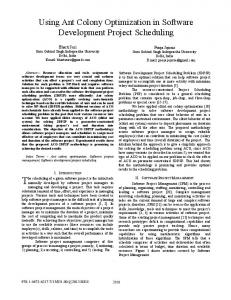
A. Function with two unknown constants RACO Algorithm has been tested on the following function with two unknown constants and : (4) and have been A number of datasets for generated using the values of and to be and respectively and 5% error. The other input parameters are: Initial ranges: No. of models ( ) = No. of models ( ) = No of cities = No of ants ( No of ants ( No of ants No of iterations

θ

Figure 1. Possible pairs of values for

and

after first iteration

(depth=1) forthefunction

(equispaced initially) .

As mentioned above, the algorithm has been allowed to run for 80 iterations for the first depth. Fig. 1ashows the plot of possible pairs of and obtained from the ant positions after 1st iteration (depth=1).It is seen that as the no of iterations increase, the ants, initially equidistant, tend to move in different directions in a way so as to accumulate at some fixed cities. Fig. 1b shows results for this function after 80 iterations. It is observed that after the first depth, two cities pass the local maxima test. They are . The further process of optimization has been carried out for more number of depths and the results are shown in table 1. We find that finally two solutions have emerged for the problem and hold equally good. The two solutions are,

With

, the characteristic function is (5)

With

, the characteristic function is

θ

Figure 2.Possible pairs of values for forfunctionthe

and

after 80 iterations (depth=1) .

B. Geophysical Problem with five unknown parameters The method has been used to solve a geophysical problem of self potential anomaly inversion. The self potential anomaly method is used to measure the naturally occurring potential differences generated mainly by electrochemical, electro-kinetic and thermo-electric sources. In some cases, it can be considered that this anomaly is due to a single polarized body assuming a model of simple geometry like a sphere, a cylinder or a thin sheet.In this example we have analyzed the case of self potential anomaly due to a inclined sheet buried inside the earth. The geophysical datasets used here are synthetic in nature. One of them is a


noise free dataset and the other is a dataset with 5% noise, both anomalies being considered to be due to a inclined sheet buried inside the earth. The SP anomaly at a point on the surface on a line perpendicular to the strike of an inclined sheet of infinite horizontal extent is given by Murthy and Haricharan [26].

(7)

In the above equation, is the depth, is the inclination angle, is the half-width of the sheet like body, is the electric current dipole moment, is the origin of the anomaly and is the SP anomaly at the point lying at distance from the origin of the anomaly. Keeping the case of inclined sheet in mind, an ideal set of values has been assigned to these parameters and then the forward model is worked out to generate the synthetic geophysical dataset. The no. of models for each parameter, no. of ants and the ideal value for each of the parameters for the case of inclined sheet are listed in table 3. From this data, the following calculation can be done:

Figure 3.Misfit curve for the ideal noise free data and calculated SP anomaly for a inclined sheet. (*) signs represent the ideal data points and the continuous line denotes the curve obtained after the inversion process.

No of cities =60 * 70 * 25 *25 * 25 = 65625000, No of ants = (equispaced) No of iterations=50 The ideal and calculated data are compared by the evaluation of misfit stated by the misfit function. The definition of the misfit function used here is as follows:

(8) Table 3 also shows the range values for each parameter, calculated value of the parameters, error and the misfit observed between the calculated dataset and synthetic dataset for the noise free data as well as the data with 5% noise. The results obtained are found to be very close to ideal values. Still better results can be obtained by increasing the extent of recursion for the method. The calculated values of the parameters have been used to generate a dataset, and both the datasets i.e. the true set and the calculated set are further used to plot the misfit curves for the noise free as well as noisy data. Figure 4a and Figure 4b are the misfit curves obtained for the noise free and noisy data respectively. From the curves, it can be inferred that RACO method is stable and works fine on the five parameter geophysical problem for smooth as well as rugged data.

Figure 4.Misfit curve for the ideal data with 5% noise and calculated SP anomaly for an inclined sheet. (*) signs represent the ideal data points and the continuous line denotes the curve obtained after the inversion process.

V. CONCLUSIONS We have modified the existing ACO technique to produce results with more accuracy. The modified algorithm, termed as RACO, has been tested on a function with two unknowns and it proves to be efficient and practicable. We also applied it to a geophysical function with and without noise and found that this method is able to find proper results for even highly rugged datasets. Several advantages of RACO method make it a better option over other global optimization techniques. Unlike some other optimization methods, RACO doesn’t demand any initial value to be assigned to each of the parameters. It searches evenly for the solution in a given range as supplied by the user. The time algorithm for RACO is far lesser than that of the general ACO method. In RACO, the ants are not placed at each and every city. Rather, they are placed at certain intervals and tend to move towards better solution. Hence, many of the cities are not checked, but are approximated from the nature of the neighbours, which leads to reduction of time


[13] J. Holland, Adaptation in Natural and Artificial Systems, Ann Arbor: University of Michigan Press, 1975. [14] I. Rechenberg, Evolutionsstrategie—Optimierung technischer Systeme nach Prinzipien der biologischen Information, Fromman Verlag, Freiburg, Germany, 1973. [15] H.-P. Schwefel, Numerical Optimization of Computer Models. John Wiley & Sons, 1981. [16] M. Dorigo and G. Di Caro, “The Ant Colony Optimization metaheuristic,” in New Ideas in Optimization, D. Corne et al., Eds., McGraw Hill, London, UK, pp. 11–32, 1999. [17] M. Dorigo, G. Di Caro, and L.M. Gambardella, “Ant algorithms for discrete optimization,” Artificial Life, vol. 5, no. 2, pp. 137–172, 1999. [18] M. Dorigo and T. Stützle, Ant Colony Optimization, MIT Press, Cambridge, MA, 2004. [19] M. Dorigo, M. Birattari, and T. Stützle, Ant Colony Optimisation, UniversitéLibre de Bruxelles, BELGIUM, 2006. [20] T. Stützle and H.H. Hoos, “Improving the Ant System: A detailed report on the MAX–MIN Ant System,” FG Intellektik, FB Informatik, TU Darmstadt, Germany, Tech. Rep. AIDA–96–12, Aug. 1996. [21] T. Stützle, Local Search Algorithms for Combinatorial Problems: Analysis, Improvements, and New Applications, ser. DISKI. Infix, Sankt Augustin, Germany, vol. 220, 1999. [22] T. Stützle and H.H. Hoos, “MAX–MIN Ant System,” Future Generation Computer Systems, vol. 16, no. 8, pp. 889–914, 2000. [23] V. Maniezzo, “Exact and approximate nondeterministic tree-search procedures for the quadratic assignment problem,” INFORMS Journal on Computing, vol. 11, no. 4, pp. 358–369, 1999. [24] O. Cordón, I.F. de Viana, F. Herrera, and L. Moreno, “A new ACO model integrating evolutionary computation concepts: The best-worst Ant System,” in Proc. ANTS 2000. [25] C. Blum, A. Roli, and M. Dorigo, “HC–ACO: The hyper-cube framework for Ant Colony Optimization,” in Proc. MIC’2001— Metaheuristics International Conference, vol. 2, Porto, Portugal, pp. 399–403, 2001. [26] B.V.S. Murthy, P. Haricharan, “Nomograms for the complete interpretation of spontaneous potential profiles over sheet like and cylindrical 2D structures”, Geophysics vol. 50, pp. 1127–1135, 1985.

complexity. Due to the nature of recursively hunting for better solution, the accuracy of results for RACO method increases with depth and hence highly accurate solutions can be obtained. For these reasons, we can say that the RACO method is a stable and efficient method and can be preferred over other optimization techniques for generating better results. REFERENCES [1]

P.-P. Grassé, Les InsectesDans Leur Univers, Paris, France: Ed. du Palais de la découverte, 1946. [2] J.-L. Deneubourg, S. Aron, S. Goss, and J.-M.Pasteels, “The selforganizing exploratory pattern of the Argentine ant,” Journal of Insect Behavior, vol. 3, pp. 159, 1990. [3] M. Dorigo, V. Maniezzo, and A. Colorni, “Positive feedback as a search strategy,” Dipartimento di Elettronica, Politecnico di Milano, Italy, Tech. Rep., pp. 91-016, 1991. [4] M. Dorigo, “Optimization, learning and natural algorithms” (in italian), Ph.D. dissertation, Dipartimento di Elettronica, Politecnico di Milano, Italy, 1992. [5] M. Dorigo, V. Maniezzo, and A. Colorni, “Ant System: Optimization by a colony of cooperating agents,” IEEE Transactions on Systems, Man, and Cybernetics—Part B, vol. 26, no. 1,pp. 29–41, 1996. [6] V. Cernỳ, “A thermodynamical approach to the traveling salesman problem,” Journal of Optimization Theory and Applications, vol. 45, no. 1, pp. 41–51, 1985. [7] S. Kirkpatrick, C.D. Gelatt Jr., and M.P. Vecchi, “Optimization by simulated annealing,” Science, vol. 220, pp. 671–680, 1983. [8] F. Glover, “Tabu search—part I,” ORSA Journal on Computing, vol. 1, no. 3, pp.190–206, 1989. [9] ——, “Tabu search—part II,” ORSA Journal on Computing, vol. 2, no. 1, pp. 4–32, 1990. [10] F. Glover and M. Laguna, Tabu Search, Kluwer Academic Publishers, 1997. [11] H.R. Lourenço, O. Martin, and T. St¨utzle, “Iterated local search,” in Handbook of Metaheuristics, ser. International Series in Operations Research & Management Science, F. Glover and G.Kochenberger, Eds., Kluwer Academic Publishers, vol. 57, pp. 321–353, 2002. [12] L.J. Fogel, A.J. Owens, and M.J. Walsh, Artificial Intelligence Through Simulated Evolution, John Wiley & Sons, 1966.

TABLE I. RANGE, NO. OF MODELS, CITIES OF LOCALIZATION OF ANTS AND ERROR IN THE CALCULATED VALUE OF THE

AND

FOR DEPTHS 1 TO 4 FOR

THE FUNCTION

Depth

Lower limit (

)

Upper limit

No of model (

Cities of localization

)

1

(0.0,0.3)

(4.0,1.3)

(51,51)

(2.0,0.52), (1.2,1.02)

(0.08, 0.02)

2

(1.92, 0.5)

(2.08, 0.54)

(11,11)

(2.0,0.524)

(0.016, 0.004)

2

(1.12, 1.00)

(1.28, 1.04)

(11, 11)

(1.152,1.048)

(0.016, 0.004)

3

(1.984, 0.52)

(2.016, 0.528)

(11,11)

(2.0, 0.5232)

(3.2e-3, 8e-4)

3

(1.136, 1.044)

(1.168, 1.052)

(11, 11)

(1.1552, 1.0472)

(3.2e-3, 8e-4)

4

(1.9968,0.5224)

(2.0032, 0.524)

(11,11)

(2.0,0.52352)

(6.4e-4, 1.6e-4)

4

(1.152, 1.0464)

(1.1584, 1.048)

(11, 11)

(1.15456,1.046880)

(6.4e-4, 1.6e-4)


TABLEII. IDEAL VALUES, RANGE, CALCULATED VALUES AND ERROR IN THE CALCULATED VALUE OF EACH PARAMETER FOR THE SP ANOMALYINVERSIONDUETO AN INCLINED SHEET BURIED INSIDE THE EARTH. BOTH, THE NOISE FREE DATA AND 5% NOISY DATA ARE USED AND THE MISFITS ARE CALCULATED. Inclined Sheet

Parameters z (in m)

á (in degrees)

Misfit

a (in m)

K (in mV)

x0 (in m)

No. of models

60

70

25

25

25

-

No. of ants

4

4

4

4

4

-

Ideal Value

10

35

5

149

8

-

Range

2-50

20-50

1-15

60-250

0-20

-

Calculated value

9.9975

34.9875

5.02666

148.20234

7.99142

Error

0.0025

0.0125

0.02666

0.79766

0.00858

Calculated value

9.9770

36.1240

5.1452

152.2310

7.8236

Error

0.023

1.124

0.1452

3.231

0.1764

Noise free data

0.00844

10% noisy data

0.01586