Recursive fast computation of the two-dimensional discrete cosine

Recursive fast computation of the two-dimensional discrete cosine transform W.-H. Fang N.-C.Hu S.-K. Shih

Abstract: An efficient algorithm is presented for computing the two-dimensional discrete cosine transform (2-D DCT) whose size is a power of a prime. Based on a generalised 2-D to onedimensional (1-D) index mapping scheme, the proposed algorithm decomposes the 2-D DCT outputs into three parts. The first part forms a 2D DCT of a smaller size. The remaining outputs are further decomposed into two parts, depending on the summation of their indices. The latter two parts can be reformulated as a set of circular correlation (CC) or skew-circular correlation (SCC) matrix-vector products by utilising the recently addressed maximum coset decomposition. Such a decomposition procedure can be repetitively carried out for the 2-D DCT of the first part, resulting in a sequence of CC and SCC matrix-vector products of various sizes. Employing fast algorithms for the computation of these CCiSCC operations can substantially reduce the numbers of multiplications compared with those of the conventional row-column decomposition approach. In the special case where the data size is a power of two, the proposed algorithm can be further simplified, calling for computations comparable with those of previous works.

1

Introduction

The DCT has found applications in various facets of signal-processing applications, ranging from transform domain adaptive filtering and the design of filter banks to speech coding [l]. The 2-D DCT, in particular, has been widely considered to be the most effective scheme for transform coding. As such, various international standards, such as the MPEG-1,2 and H.261, have incorporated the 2-D DCT as the imageivideo coding ingredient block. To facilitate real-time implementations, the development of efficient algorithms for computing the 2-D DCT has been of great interest over the past few decades. The conventional approach for computing the 2-D DCT is based on the row-column decomDosition 0IEE, 1999 IEE Proceedings online no. 19990021 DOI: 10.1049/ip-vis:19990021 Paper first received 5th May and in revised form 26th October 1998 The authors are with the Department of Electronic Engineering, National Taiwan University of Science & Technology, Taipei, Taiwan, Republic of China IEE Proc-Vis. Image Signal Process., Vol. 146. No. 1. February 1999

method, which first determines the row (column) transforms of the input 2-D data, then transposes these intermediate results, and finally takes the column (row) transforms of the transposed data. More efficient algorithms can, in general, be attained by working directly on the 2-D data by fully exploiting the 2-D characteristic of the kernel function. For example, Cho and Lee addressed a fast algorithm which decomposes an N x N DCT into N 1-D N-point DCTs [2], in contrast to the 2N N-point DCTs required for the row-column approach. Duhamel and Guillemot considered an efficient polynomial transform-based approach [3, 41. Wu and Paoloui proposed a recursive 2-D DCT algorithm [5] that extended Hou's work [6]. Kung and Lee considered a convolution-based algorithm that admits efficient hardware implementations [7]. Despite their efficiency, these fast algorithms, however, are only applicable to the 2-D DCT of size 2' x 2'. In this paper, we address a new fast algorithm for the recursive computation of the 2-D DCT of size p' x p', where p is a prime. The essence of the new algorithm is based on the 2-D to 1-D index mapping scheme, as addressed in [8]. This index mapping scheme has successfully been applied to the fast computation of the 2D generalised discrete Hartley transform. A similar technique was also utilised to compute the 2-D discrete Fourier transform using the discrete Randon transform (or linear congruence) [9]. Based on this index mapping scheme, the proposed algorithm decomposes the 2-D DCT output components into three parts. In the first part, the output components whose indices are multiples of p form a pr-' x pr-' DCT. The remaining output components are further decomposed into two parts, depending on the summation of their indices. The latter two parts can be reformulated as a set of CC or SCC matrix-vector products by utilising the recently proposed maximum coset decomposition [lo, 111. Such a decomposition procedure can be repetitively carried out for the 2-D DCT of the first part by following the same steps. As a consequence, the Computation of the 2-D DCT is converted into a sequence of CC and SCC matrix-vector products of various sizes. Employing fast algorithms for the computation of these CCiSCC operations, we can thus substantially reduce the numbers of multiplications required, compared with those of the row-column decomposition approach. In the special case when p = 2, the proposed algorithm can be further simplified, calling for computations comparable with those of previous works. 2

Fast algorithms for computing the 2-D DCT

For a set of 2-D data {x(k,,k2);0 < kl I N - 1, 0 I k2 - 1 }, the 2-D DCT is defined as

5N

25

depending on whether n1 + n2 is even or not. Thereby, X ( n l , n2) can now be rewritten as n X'(n1,nz)= Y ( n )

x cos

4N

(1) for 0 I n l , n2, 2 N - 1, where the scale lactor, without loss of generality, has been left out for notational brevity, and N = pr with p being a prime. Invoking the trigonometric identity of cos(a) cos(p) = 'i2[cos(a + p) + cos(a - p)], we can rewrite eqn. 1 as

1 X ( n 1 , n z ) = 5 [ X + ( n z , n 2 )+ x - ( n l , n 2 ) ]

(2)

where

k1=0 k2=0

cos (27r[(2kl

+ 1)nl + (2ka + l )n 2 ] 4N (3)

and N - 1 N-1

x(h,b)

X-(nl,nz) = kl=O kz=O

cos (27rPkl

+ 1)nl

-

(2k2

+ l)n2]

4N

1

(4) Using the 2-D to I-D index mapping equations of 181, (2k1 1)nl f (2k2 l)n2 E (2n 3)25 mod 4N if n1 + n2 is even (5)

+

+

+

( 2 k l + l ) n l f ( 2 k 2 + 1 ) n a E (2n+1)(25+1) mod 4N

otherwise (6) Xi-(nl, n2) and X-(nl, n2) can then be evaluated, respectively, using the following I-D expressions: X+(YL1,722)

6 Y+@)

otherwise

(7) and X'-(n1,n2)

-I -

a

= Y-(n)

if

n1

+ n2 is even

otherwise

(8) where y'(k) = X k 2 x(k,, k2), in which (kl, k2) satisfies the index mapping equations of eqn. 5 or eqn. 6, 26

1 7-

-

=

1

I

y(k) cos

(

if

n1

+ 122 is even

(sa)

2Qn+ll(2k+1))

k=O

otherwise (9b) where Y(n) 1/2[Y+(n) + Y-(n)] and y ( k ) k 1 / 2 b C ( k+) y-(k)].Next, we address the issue of solving the 2-D to I-D index mapping equations (eqns. 5 and 6). To solve these, n l , n2 and n must be decided first. In other words, the index ( n l ,n2) of the 2-D output component is first mapped to a predetermined I-D output component with an index n, denoted by (nl, n2) + n. According to this (nl, n2) + 12, a solution set of ( k l ,k 2 ) on the left-hand side of eqns. 5 and 6 can thus be obtained for every specific k on the right-hand sides of eqns. 5 and 6. y ( k ) can then be determined by a summation of x ( k l , k2) of these corresponding ( k l ,k2)s. To mitigate the overhead in the computation of y(k), we consider those { X ( n l ,n 2 ) } that share the same set of { y ( k ) } together. As all of the corresponding (nl, n2)s satisfy the congruence eqns. 5 and 6, they are related to each other by some factors. Therefore, if one of these indices, say ( n ? , n ; ) , + 0, then the other indices (nl, n2)s inside this set can be determined as a function of (n?, n ; ) and n. Such a particular (n!, n!) is thus referred to as a dominant point for the corresponding set of { X ( n , , n 2 ) } . Then, as shown in the Appendix, it follows that the rest of { X ( n l , n 2 ) } , which share the same set of { y ( k ) } ,are related to Y(n), n = 1, 2, ..., ( N - 1)/2 1, by ~

+

+

Y(72)= x (((2n l)n?),((an 1)ni)) (10) where ( . ) stands for either mod 4N or mod 2N, depending on whether eqn. 5 or eqn. 6 is employed. Note that, as both 4N and 2N are even for all N , it is easy to justify that, if a dominant point ( n y , n ! ) has a summation of indices ny + 1202 that is even(odd), then the corresponding { X ( n l ,n2)}has summations of indices n l + n2 that are all even(odd). Some output components, however, appear repetitively for different dominant points, if (2n + 1 ) is a multiple of p . For example, if N = 9 and for the dominant point (1, 1) -+ 0, we obtain a corresponding output component set as Y(0) = X(1, l), Y(1) = X(3, 3), Y(2) = X ( 5 , 5 ) and Y(3) = X(7, 7). On the other hand, the dominant point (1, 5) 4 0 will generate another output component set as Y(0) = X(1, 5 ) , Y(1) = X(3, 3), Y(2) = X(5, 7), and Y(3) = X(7, 1). We can note that X(3, 3) is repetitively computed, thus increasing the computational load. To avoid this redundant coniputation, n that satisfies (2n + 1) = mp, or equivalently, when both indices of the outputs are multiples of p owing to eqn. 10, will be treated separately. Given this fact, along with the index mapping eqns. 5 and 6, we can classify the computation of the 2-D DCT in the following three categories, according to the output indices: Part I : {X'(nl, n2):n1 m o d p = n2 m o d p = 0} Purt 2: { X ( n l ,n2):n l mod p # 0 or n2 mod p # 0, nl + n2 is even) IEE Proc -VIS Image Signul Process Vu1 146 N o I Fehrirarr IYYY

Part 3: { X ( n l , n2):n1 mod p n2 is odd)

f

0 or n2 mod p

f

0, n1 +

For the output components of part 2, using the maximum coset decomposition as addressed in [lo, 111, the corresponding 2n + 1 (2n + 1 # mp) can be obtained by a generator that is an odd prime. More specifically, such a set of numbers can be generated by a power of g mod 2N as GI = (go, g ' , ..., ga-'} mod 2N, where g is the coset generator with order A that satisfies cos(2d 4N) = f cos(2ngr/4N) Therefore, for every dominant point, there are only A (non-redundant) corresponding Y(n)s (or, equivalently, X ( n l , n2)s),where A = pr-' (p 1)/2, if N = p' [12]. Also, the (N + 1)/2 input points in eqn. 9a can be divided into the following cosets: GI, G2 = pG1 = (p, pg, ..., pgmp'pl}mod 2N, ..., G, = pr-'G1 mod 2N, and G,,, = {N}. The corresponding orders of these cosets are A, Alp, ..., and 1, respectively, and their summation is equal to A + Alp + ... + 1 = (N + 1)/2. By replacing (2n + 1) and k with f and p'gl, respectively, in eqn. 9a, we can rewrite eqn. 9a with ( N + 1)/ 2 inputs and A outputs as

((v))

Along the same line, the computation of the output components of part 3 can be simplified by following the above steps, except that the operation of mod 2N is replaced with mod 4N. More specifically, for every dominant point, the corresponding 2n + 1 can be generated by a generator g mod 4N as GI = (go, g', ..., ga-l} mod 4N, where g is the coset generator with order A. The ( N - 1)/2 input points in eqn. 9b can thus be divided into the following cosets: GI, G2 = pG1 = (p, pg, ..., pgUp-'} mod 4N, .., and G, = p"GI mod 4N. The corresponding orders of these cosets are A, ..., and AlW-l),respectively, and their summation is equal to A + Alp + ... + Alpr-l = ( N - 1)/2. By replacing (2n + 1) and (2k + 1) with gm and p'g', respectively, in eqn. 9b, we can rewrite eqn. 9b with ( N - 1)/2 inputs and A outputs as 77

f /gm

-

1\\

(13) where m = 0, 1, ..., A 1 and ( . ) denotes mod 4N operation. As above. we can also exmess ean. 13 as the following matrix notation: -

(11) where m = 0, 1, ..., A - 1, and ( . ) denotes mod 2N operation. Expanding eqn. 11 yields the following more illustrative matrix notation:

... ... ... ...

=c i=O

X

r

X

(14) where & cos((2&)/4N), and we have used the fact that CppP1trn = - Cplp, i = 0, ..., r , rn = 0, ..., A - 1. As such, the computations of the 2-D DCT outputs in part 3 can be implemented by a sequence of SCC matrixvector products of sizes Alpi, i = 0, ..., r. Likewise, the input and output indices are required to be relocated if they are outside the range. If ( ((pigm) 1)/2 ) < (N 1)/2, then the input is y(((pig") - 1)/2); on the other hand, if ( pig" ) 2 (N - 1)/2, we will use the input as -y(N - ((pig"))/2) in eqn. 9b. Also, if ( (g' 1)/2 ) < N, the output of eqn. 9b is Y(( (g' 1)/2 )); otherwise, the output will become -Y(n) or Y(n), depending on whether ( g' ) can be expressed as 2N f (212 + 1) or 4 N - (2n + 1).

ck

where C, 6 cos(2nk/2N) and we have used the fact that CpigUp'+m= C( i2n, i = 0, ..., r, m = 0, ..., A - 1. AS such, the computation of the 2-D DCT output components in part 2 can be implemented by a sequence of CC matrix-vector products of sizes Alpi,i = 0, ..., r . Note that, as 0 I ( g" ) mod 2N, some rectifications are made for the y(k) in eqn. 9a. If ( pign7) < (N + 1)/2 then we simply use y(( pig" )); on the other hand, if (pig") 2 (N + 1)/2 we will use -y(N - ( pig" )), as readily justified using eqns. 5 and 6. Similarly, if ( g' ) < N, the output of eqn. 9b is Y(( (g' 1)/2 )); otherwise, the output will become -Y(n), where ( g i) = 2N (2n + 1). -

-

IEE Proc.-Vis. Image Signal Proress.. Vol. 146. No. I , February 1999

-

-

-

Ll

From the above discussion, we can note that the algorithm initially requires (N2(P2- l))/p2il dominant points that, in turn, generate a total of N2(1 l/p2) output points. Such a decomposition procedure can be recursively carried out for the 2-D DCT of part 1. The overall steps can be summarised as the following algori thm for computing the 2-D DCT of size p r x p r (with initial value i = 1): Srep I : Divide the output components into three parts, according to their indices. If both of the indices nl and n2 are multiples of p (part l), these {X(nl, n2)) form a 2-D DCT of size pr-' x pr-'. The rest of the output components can be further classified into two parts, part 2 and part 3, depending on whether the summation of nI/@'-l) + n2/(pi-')is even or odd, respectively. Step 2: The { X ( n l ,n2)}in parts 2 and 3 can be further classified into several groups with different choices of dominant points. Every group of {X(nl,n2)}in parts 2 and 3 can be implemented using the CC operation of eqn. 12 and the SCC operation of eqn. 14, respectively. The resulting output components can be obtained by using the index mapping scheme of eqn. IO. The pr-' x pr-' DCT of part 1 can be further decomposed along the same steps by going back to step 1, with i = i + 1 until i = Y. As a special case when p = 2, eqn. 9a and b can be simplified as

efficiently implemented via the algorithm of [IO], with y ( k ) as the input and the odd-indexed output components as the corresponding output. To follow, we consider two examples to reinforce the proposed algorithm. Example 1 ( 5 x 5 DCT): As N is equal to 5 (p = 5 and Y = 1) in this example, there are N2(1 - lip2) = 24 output components to be determined in the first iteration. If we choose the generator g = 3, the corresponding order ilcan be easily found to be 2. This implies that a total of 12 dominant points, which can be (arbitrarily) chosen as (0, l), (1, 0), (1, 2), ( I , 4), (4, I), (4, 31, (0, 21, (1, I), (1, 31, (2, 01, (2, 2) and (2, 41, are required. Then, we determine the corresponding { y ( k ) } for the above dominant points by using the index mapping schemes of eqns. 5 and 6. For the dominant points (0, 2), (1, l), (1, 3), (2, 0), (2, 2) and (2, 4), as the index summations are even, eqn. 5 is employed. As an example, for the dominant point (1, l), y ( k ) = 1/2b+(k) + y-(k)],k = 0, 1, 2, where y+(k) and y-(k) can be determined using eqn. 5 as follows: y'(0)

= - .r(0,4) - x(1,3) - ~ ( 2 . 2) ~(3.1) - X(4,O)

y-(0) = + 5 ( 0 , 0 ) + z ( l , l ) + 2 ( 2 , 2 ) +2(3.3)

+ J44,4) y'(1)

= +z(O,O) -

- x ( 0 , 3 ) -.r(1,2) -z(1.4)

X ( 2 , l ) - 5(2,3) - 2(3,0) - 4 3 . 2 )

- 2(4,1) + 2(4,4) + + z(1,O)+ ~ ( 1 , 2 ) + Z(2,l) + 2(2,3) + 2(3,2) + 2(3,4) 2(4,0) + z(4,3) y+(2) = + Z ( 0 , l ) z ( 0 , 2 ) + Z(1,O) - z(1,l)

~ ~ (= 1 )~ ( 0 , l ) 2(0,4) otherwise (15) Employing the maximum coset decomposition as discussed above, we can obtain

-

-

- 42,O) -

))?((I

44.2)

-

2(2,4) - 2(3,3) + 4 3 . 4 )

+ 2(4,3)

~ ~ ( =2 +) ~ ( 0 . 2 -~c(O,3) ) + ~ ( l , 3 -)~ ( 1 , 4 )

+ 4 2 . 0 ) + c(2,4) - 44.1)

if n; + 722 = even

(16)

and

k'

((?))

A-1

=

CY ( ( P 2 S r n ) )cos (27rpzg 4N

)

1 =O

(17) where m = 0, ..., A - 1, and ( . ) denotes mod 2N and 411' in eqns. 16 and 17, respectively. As above, eqns. 16 and 17 can be implemented using a sequence of SCC matrix-vector products. These SCC operations can be otherwise

-

z(3,O)

+ 2(4,2)

+ z(3,l)

An illuminative picture to demonstrate the above computation is shown in Fig. 1. For every one of these dominant points, the corresponding { Y(n)}, which shares the same { y ( k ) } ,can be determined using the CC matrix-vector product of eqn. 12, as follows:

I.'(O)

[

cos+

[1'(1)1 =

cos5

y(1)

]

4 2 )

%

+ [cos I [-Y (0)l (18) The resulting { X ( n l , n2)} can then be determined using eqn. IO. Following the above for the dominant

r

28

IEE Proc.-Vi.s. Imuge Signal Process.. Vol. 146, No. 1. Fehruury 1999

point (1, l), we obtain

Y ( 0 )= X(n(:,ni> = X(1,l)

x

Y ( l ) = ( ( 3 4 , ( 3 n i ) )= X ( 3 , 3 ) Similarly, for the dominant points (0, l), (1, 0), (1, 2), (1, 4), (4, 1) and (4, 3), eqn. 6 should be employed to determine { y ( k ) } .For every one of these dominant points, the corresponding { Y(n)}, which shares the same { y ( k ) } ,can be determined using the SCC matrixvector product of eqn. 14, as follows: (19) The resulting outputs {X(nl, n2)) can then be obtained using the index mapping eqn. 10. In the

second iteration, there is only one output component, i.e. X(0, 0), that needs to be determinedd-,which can be easily determined by X(0, 0) = CC:,, C k , = , x(k,,k2).A butterfly-like structure depicting the above computing procedure is shown in Fig. 2 . Example 2 (4 x 4 DCT): As N is equal to 4 (p = 2 and r = 2) in this example, there are N2(1 - l/(p2))= 12 output components to be determined in the first iteration. If we also choose the generator g = 3, the corresponding order d can be easily found to be 2. This implies that a total of six dominant points, which can be (arbitrarily) chosen as (0, l), (1, 0), (1, 2), (2, l), (1, 1) and (1, 3 ) , are required. For the dominant points (1, 1) and (1, 3), the index summations of the associated { X ( n l ,n?)} are even, and } be determined using the the corresponding { Y ( M ) can

29

CC matrix-vector product of eqn. 12, as follows:

prime. lJsing the same trigonometric identity, eqn. 24 can be rewritten as 4kl.k2)

whereas, for the dominant points (0, I), (1, 0), (1, 2) and (2, l), the index summations of the associated f X ( n , , nz)} are odd and the corresponding { Y(n)} can be determined using the SCC matrix-vector product of eqn. 14, as follows

=

1 N-l

N-l

5

X(k1,ka)

n1=0 n2=0

x cos

27r [ ( a h

(

+ l)n1 + (2k2 + l ) n 2 ]

)

4N

1 IV--l N-l

+5

X(kl,k2)

n1=0 n2=0

In the second iteration, three output components, namely X(0, 2), X(2, 0) and X(2, 2), can be determined by

[Y(O)I = Y ( 1 )

(22)

and

y

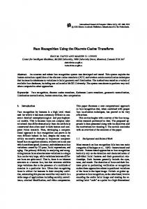
[Y(O)I= [cos 1 [!@)I (23) In the third iteration, X(0, 0) can be easily obtained by the summation of all inputs {x(k,,k 2 ) } .A butterflylike structure depicting the above computing procedure is shown in Fig. 3 .

x cos

(

27r [(2k1

+ 1)nl - (2k2 + l)n.L]

)

4N

(25) Using a modified 2-D to I-D index mapping equation, as follows: ( 2 k l 1)nl f (2k2 l)nz ( 2 k 1)2n mod 4 N (26) we can re-express eqn. 25 as

+

+

+

z ( h , k 2 ) = y(k) A‘-1

Y1(n)cos

= n=O

~ ( 0 . 0-)x(3,O)

Xi1,O)

xiO.3)- x(3,3)

X(3.0)

x (1,I 1- x ( 2 3 1

X(1,2)

x(1,2)- x12,2)

-X(3,21

xl0,l)- ~ ( 3 . 1 )

X(1,I)

xi0,2) ~ ( 3 . 2 )

x (3.3)

x(1.0)- X(2,O)

X(1,3)

~ ( 1 , 3 )xi2,3) -

+

N-1

Yz(n)cos n=O

(27) where Y1(21 = Cn2 X(nl, nz) in which ( n , , n2)s satisfy the index mapping equation of eqn. 26 with plus(minus) sign. Employing the maximum coset decomposition scheme addressed above, eqn. 27 can be rewritten as

-X(3,1)

((V))

x(O,O)+x(3,0) x(0,3)* x (3,3) xil,l)* x (231 xi1,2)* x(2,2) x(1,Ob x (2.01

x(1,3)* x(2,3) xlO,l)* ~ 1 3 . 1 ) x(0,2)+ x (3,21

X(2,I) -X (2.3)

x (0.2)

=

X(2.0) X(0,O)

Fig.?

algorithm

........ X(2,2) Structure for computing the 4 x 4 DCT by using proposed fast

(28) Expanding eqn. 28 into a matrix form, we can note that the computation of { y ( k ) }is equal to a summation of CC and SCC matrix-vector products, such as those of eqns. 12 and 14, respectively. In a similar manner, the resulting {x(k,,k 2 ) } can then be obtained from { y ( k ) } using the index mapping, as follows:

For the computation of the 2-D inverse DCT (IDCT), the fast algorithm addressed above can also be employed, with slight modifications. The 2-D IDCT for the transformed data { X ( n l ,n2)}is given by

Y@) = x

((

((2k

+ 1)(2kY + 1))- 1 2

(((2k

>-

+ 1)(2k! + 1)) 2

-

>>

1

(29) where (k’i, k!) is the chosen dominant point, and ( ) denotes mod 2N operation. 3

(24) for 0 5 k l , k2, 5 N - 1, where the scale factor has again been left out for brevity, and N = p‘ with p being a 30

Comparison and discussion

In this Section, we compare the computational complexity of the proposed fast algorithm with that of existing ones. Because the algorithm recursively IEE PIOL-Vis Image Signal ProceJh

Vol 146 No I Fehrrrarr 1999

computes the 2-D DCT of size N x N ( N = pr), it is straightforward to justify that the numbers of multiplications MUL(N) and additions ADD(N) are

and

ADD(N) =

IN

T-2

l5

z=o

+-2 xN2 2

3N (=log,

N

);

-

2J log, (E4 3x

--

4x22

2j

j=o

+N2(log2N

+4

r-I

r-1

2=2

z=1

+ 1)+ c(2'-)'

2pz

+4

(33)

r-i-I

x

j=O

A

-

-

pr-j-l

'

I

I J

-

'

\

pr-l

(

J

+N(3+:)-2 (31)

respectively, where Mcc(m) (Acc(m)) and Mscc(m) (Ascc(m)) stand for the numbers of multiplications (additions) required for the CC and SCC matrix-vector products of size m, respectively. Table 1: Comparison of row-column decomposition approach with proposed one for computing Algorithms

Complexity

3x3

5x5

7x7

Row-column

number of multiplications

18

50

112

180

number of additions

24

130

420

612

8

30

64

80

27

169

523

1059

Proposed

number of multiplications number of additions

9x9

In the special case where p = 2, the recursive equations for computing the required numbers of multiplications and additions can be simplified, respectively, as (32)

Table 1 provides the numbers of multiplications and additions required for computing the p r x p r (JJ is an odd prime) DCT using the proposed fast algorithm and the row-column decomposition approach, whereas other existing fast algorithms are only applicable to p = 2. The 1-D DCT algorithms used in the row-column decomposition approach are based on the ones of [6], when p = 2, and of [13], when p is an odd prime, whereas the CCiSCC matrix-vector products employ the algorithms of [14]. In Table 2, we also compare the computational complexity with other existing fast algorithms when p = 2. As we can observe from Table 1, the proposed algorithm requires fewer numbers of multiplications (at the price of more additions), compared with those of the row-column decomposition approach. In the special case when p = 2, we can note from Table 2 that the proposed fast algorithm calls for the same numbers of multiplications and roughly the same numbers of additions as those of [2, 41, which are known to be by far the most parsimonious approaches. As a whole, the proposed fast algorithm possesses the following advantageous features: (a) The new algorithm is more general than the previous ones in that it is also applicable to the 2-D DCT of size p" x p r , where p is any prime. Although the current standards are based on the 2-D DCT of power-of-two data size, it has been observed that using a 2-D DCT of general data size can reduce the annoying blocking effect in the DCT-based image coding problems; see, for example, [15] for a discussion on lapped transforms. (b) In contrast to the row-column decomposition approach, the new one does not require the transposition manipulation. In addition, the outputs corresponding to every dominant point can be computed independently, thus allowing for efficient parallelipipelined implementations. (c) The 2-D to I-D index mapping scheme employed can be readily extended to the higher-dimensional case. In contrast, the previous ones, as addressed in [2, 161, are specifically designed for the 2-D DCT and do not allow for any extension.

Table 2: Comparison of various fast algorithms for computing 2' x 2' DCT Algorithms

Row-column

[31

Data size

Mult.

Mult.

Add.

I21 Add.

[I61

Mult.

Add.

Proposed

Mult.

Add.

Mult.

Add.

4x4

32

74

16

68

16

74

16

74

16

74

8x8

194

464

96

484

96

466

112

472

96

466

1 6 x 16

1024

2592

512

2531

512

2530

640

2624

512

2530

32 x 32

5120

13376

2560

12578

2560

12738

3328

13504

2560

12738

64 x 64

24576

65664

12288

60578

12288

61314

16384

66174

12288

61314

~~

IEE Proc-Vis. Imuge Signal Process.. Vol. 146, No. 1, February 1999

~

~~

~~

~

31

4

Conclusions

In this paper, we propose a new fast algorithm for the recursive computation of a p r x p r DCT, where p is a prime. The algorithm recursively decomposes the output components into three parts according to their indices. Such a classification of outputs can, in turn, be reformulated as a set of CC and SCC matrix-vector products of various sizes. Utilising existing fast algorithms for the computation of these CC and SCC matrix-vector products, we can thus obtain an algorithm with minimum multiplicative complexity. A similar fast algorithm for computing the 2-D IDCT is addressed as well. 5

Acknowledgments

This research was supported by the National Science Council of the Republic of China, under contract NSC87-2213-E-011-014. The authors would like to thank the reviewers, whose comments have enhanced the quality and readability of this paper. 6

= (2n+l)(2k+l)

mod 4 N otherwise (35) The negative case of eqn. 10 follows straightforwardly. We begin our discussion with eqn. 34. Recall that the solution of a linear diophantine equation alxl + 4 x 2 == b can be expressed by the following parametric expression: a2 q ( t ) = q ( 0 ) -t (36) d (2kl+l)n1+(2k2+l)n2

+

a1

Q ( t ) = 22(0) - -t (37) d where xI(0) and x2(0) are particular solutions, d is the greatest common divider (GCD) of al and a*, and t is an integer. As ( n ; , n i ) is now a dominant point with n = 0, from eqn. 5 the indices k l , k2 and k need to satisfy the following expression:

+

+

+

(251 l)n: (2k2 l ) n i = 25 mod 4 N ( 3 8 ) A particular solution kl(0) and k2(0) to eqn. 38 can be easily determined by choosing k l ( 0 ) = 0 and then solving eqn. 38 for k2(0),as follows:

References

1 RAO, K.R., and YIP, R.: ‘Discrete cosine transform’ (Academic Press, San Diego, CA, 1990) 2 CHO, N.I., and LEE, S.U.: ‘Fast algorithm and implementation of 2-D discrete cosine transform’, IEEE Trans. Circuits Sysf., 1991, 38, (3), pp. 297-305 3 DUHAMEL, P., and GUILLEMOT, C.: ‘Polynomial transform conmutation of the 2-D DCT’. Proceedines of IEEE international confkrence on Acoust., speech, signal uprocessing, ICASSP90, Albuquerqe, NM, April 1990, pp. 1515-1518 4 DUHAMEL, P., and GUILLEMOT, C.: ‘A polynomial-transform based computation of the 2-D DCT with minimum multiplicative complexity’. Proceedings of IEEE international conference on Acoust.. speech, signal processing, ICASSP’96, Atlanta, GA, May 1996, pp. 1347-1350 5 WU, H.R., and PAOLOUI, F.J.: ‘A two-dimensional fast cosine transform algorithm based on Hou’s approach’, IEEE Trans. Signal Process.. 1991, 39, (2), pp. 544546 6 HOU, H.S.: ‘A fast recursive algorithm for computing the discrete cosine transform’, IEEE Trans. Acoust. Speech. Signal Process., 1987, 35,(IO), pp. 1455-1461 7 KUNG, S.S., and LEE, M.H.: ‘An expanded 2-D DCT algorithm based on convolution’, IEEE Trans. Consum. Electron.. 1993, 39, ( 3 ) , pp. 159-165 8 HU, N.-C., and LU, F.-F.: ‘Fast computation of the two-dimensional generalized Hartley transforms’, IEE Proc. Vis.Image Signal Process., 1995, 142, (I), pp. 35-39 9 GERTNER, I.: ‘A new efficient algorithm to compute the twodimensional discrete Fourier transform’, IEEE Truns. Acoust. Smech Sipnal Process., 1988, 36. (7). DP. 1036-1050 10 HU, N.-e.., and LIN, K.-C.: ‘Skew~~rcular/circular correlation decomposition of prime-factor DCT’, IEE Proc. Vis. Image Signal Process.. 1995, 142, (4), pp. 241-246 11 HU, N.-C., and LOUH, S.-W.: ‘Two-stage decomposition of the DCT’, IEE Proc. Vis. Image Signal Process., 1995, 142, ( 5 ) , pp. 3 19--326 12 McCLELLAN, J.H., and RADER, C.M.: ‘Number theory in digital signal processing’ (Prentice-Hall, Englewood Cliffs, NJ, 1979) 13 HEIDEMAN, M.T.: ‘Computation of an odd-length DCT from a real-valued DFT of the same length’, IEEE Trans. Signal Process., !992, 40, (l), pp. 5 4 6 1 14 NUSSBAUMER, H.H.: ‘Fast Fourier transform and convolution algorithms’ (Springer-Verlag, New York, 1982) 15 MALVER, H.S.: ‘Signal processing with lapped transforms’ (Artech House, Norwood, MA, 1992) 16 CHO, N.I., and LEE, S.U.: ‘A fast 4 x 4 algorithm for the recursive 2-D DCT’, IEEE Trans. Signal Process., 1992, 40, (9), pp. 216G2173

7

Appendix

In this Appendix, we show the index mapping eqn. 10. For brevity, we only prove

(2kl

32

+ l)nl + (252 + l)n2 E (an + 1)2k mod 4 N if n1 + 122 even (34)

where I is an integer. Employing eqns. 36 and 37, we can then obtain the general solution of eqn. 34 as

2 4 k l ( t ) = -t d

+

ny - n: 4 N l 2nY - -t (41) d 2 4 where d = GCD(2n7, 2n!), and we have used the particular solution k2(0)of eqn. 39. Plugging the solutions k l ( t ) and k2(t) of eqns. 40 and 41, respectively, in eqn. 34 and comparing both sides, we can obtain k2(t) =

2k

-

( 2 n l ) ( 2 n i ) t- (2n2)(2n?)t= o

(42)

and

n? (43) It then follows that, for the outputs whose indices ( n l , n2)s satisfy n1

z (an

+ l)ny

mod 2 N

(44)

and

+

122 ( 2 n l)n: mod 2 N (45) then these ( n l ,n2)s share the same { y ( k ) } . Similarly, when n1 + n2 is odd, eqn. 35 is employed. We can also (arbitrarily) choose a particular solution as kl(0) = 0 and k2(0) = (2k + 1 - ny n! + 4Nr>/2n;, where I is an integer. Then, we can determine the general solution to eqn. 35 as ~

an: k , ( t ) = -t d

and

+

2k - ny - ni 4N1 2nf - -t (46) 2 4 d Substituting eqn. 46 into eqn. 35 and equating both sides yields

kZ(t) =

( 2 n l ) ( 2 n i ) t- ( 2 n 2 ) ( 2 n y ) t= o

(47)

IEE Proc.-Vis. Image Signal Process., Vol. 146, Nu. 1 . February 1999

and

It then follows that, for the outputs whose indices (n,,n2)s satisfy

IEE Proc-Vis. Image Signal Process., Vol. 146, No. I , February 1999

n1 G

(2n

+ 1)n:

mod 2N

(49)

then these (n,,n2)s share the same { y ( k ) } .Thus it completes the proof.

33