Recursive Implementation of Anisotropic Filters. Zeyun Yu. Department of
Computer Science,. University of Texas at Austin. Abstract. Gaussian filter is
widely ...
Recursive Implementation of Anisotropic Filters Zeyun Yu Department of Computer Science, University of Texas at Austin
Abstract Gaussian filter is widely used for image smoothing but it is well known that this type of filters blur the image features (e.g., edges). Two extensions of Gaussian filters will be discussed in this survey. One is the anisotropic filtering (bilateral filtering or PDE-based anisotropic diffusion) for feature-preserving smoothing and the other is the recursive implementation of various filters that can largely reduce the computational time in certain conditions. We will also discuss the combination of anisotropic filtering and recursive implementation for image smoothing such that the anisotropic smoothing could be done in a fast way.
1. Introduction Noise is commonly seen in many types of images (for example, biomedical images and remote sensing images). It is in a great demand to smooth the images before other tasks could be conducted. Gaussian lowpass filtering is known to be an efficient and simple way for image smoothing. However, it is well known that Gaussian filtering blurs the image edges while smoothing image noise. The reason is that Gaussian filters are isotropic in the sense that all surrounding pixels affect the center pixel in a similar fashion regardless their intensity variations. Hence, the edges and the noise are treated in the same way, which yields noise reduction as well as edge blurring. An example of such effect can be seen from Fig. 1 (b). To remedy the problem of traditional Gaussian filtering, people have proposed lots of methods, trying to achieve the goal of feature-preserving smoothing. All of these methods are called anisotropic filtering and can be grouped into two categories. One is called Bilateral Filtering [7, 12, 13], which is a straightforward extension of Gaussian filtering. The other is a PDE-based technique, called anisotropic heat diffusion [4, 8]. We shall see more details on the various techniques on these topics in the following sections. In Fig. 1 (c),
we show an example of bilateral filtering on the same noisy image. We can clearly see the difference between the isotropic filtering and the anisotropic filtering. Obviously the latter one gives better results. Another important issue regarding image filtering is the implementation of the various filters. Gaussian low-pass filtering can be implemented by direct convolution, which is further accelerated by FFT. Anisotropic filters, however, are generally much more time-consuming although some authors studied fast algorithms for bilateral filtering [12]. Another fast way for implementing Gaussian filtering is by recursive scheme [5, 6]. Recursive implementation requires a constant and small number of MADDs (multiplications and additions) regardless the size of the neighborhood being considered. Hence, the time complexity of recursive implementation of Gaussian filtering is quite small compared to other sequential algorithms of Gaussian filtering [5]. However, the recursive scheme was originally designed for isotropic Gaussian filtering and little work has been done on combining the recursive scheme and the anisotropic filtering. In this project our goal is to explore the possibility of applying the recursive implementation technique on the anisotropic filtering. This survey is organized as follows. We shall begin in next section by reviewing various techniques for anisotropic image smoothing. Then in Section 3, we shall give a brief description of various recursive techniques that have been seen in literatures. In Section 4 we will see some previous work that combines the recursive techniques and anisotropic filtering and our proposed approach will be briefly described in Section 5. Finally we give our conclusion in Section 6.
Original Noisy Image
Isotropic Filtering
Anisotropic Filtering
Figure 1 Example of isotropic (Gaussian) filtering and anisotropic filtering on a medical image.
2. Anisotropic Filters Anisotropic filtering is generally represented in two different ways. One is by bilateral filtering [7] and the other is by PDE-based anisotropic heat diffusion [4]. In the following we will describe both ways one by one and later on the close relationship between these approaches will be shown. The bilateral filtering [7] is a straightforward extension of Gaussian low-pass filtering. As we know, the Gaussian filtering is defined by a function as follows:
g ( x, y ) =
1 2πσ
2
e
−
x2 + y 2 2σ 2
,
(1)
where σ is a given value, known as standard deviation. It is obvious that this function is isotropic with respect to the center. Therefore, a direct use of this function on the noisy images will result in blurred edges since this function only considers the spatial information without considering the image information around the center. The basic idea of bilateral filtering is to add an additional term to the weighting function in (1) such that the image information is taken into account:
g ' ( x, y ) = e
−
x2 + y2 2σ d
2
×e
−
( f ( x , y ) − f ( 0 , 0 )) 2 2σ c 2
,
(2)
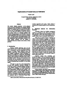
where σ d and σ c are preset parameters. The example in the following figure, reproduced from [12], shows the difference between the Gaussian filtering (shown in (b)) and the bilateral filtering (shown in (d)).
(a)
(b)
(c)
(d)
Figure 2 Illustration of bilateral filtering [12]. In (a) we show an example of noisy image and the spatial kernel (Gaussian) function g(x, y) is shown in (b). The image-related weighting function (second term in g’(x, y) ) is shown in (c). The combined weighting function g’(x, y) in (d) shows an anisotropic property.
Recently a fast implementation of bilateral filtering was proposed by Durand et al [12]. They accelerated the bilateral filtering by using a piecewise-linear approximation in the intensity domain and appropriate subsampling. Elad [13] discussed the bilateral filtering from a linear algebra point of view and pointed out some possible ways to improve it. Another commonly seen technique to realize anisotropic filtering is defined by heat diffusion equations. The first model about the anisotropic diffusion is well known as Perona-Malik model as seen in [4]. PeronaMalik model is defined by a non-linear PDE heat diffusion as follows [4]:
∂u = div( g ( ∇u )∇u ) ∂t
(3)
where g(.) is a positive non-increasing function which suppresses diffusion around image edges where the norm of the gradient is high. A common choice for g(.) is given by
g (s) = e
−
s2 K2
(4)
where K is a preset constant. Strictly speaking, however, Perona-Malik model is not an anisotropic diffusion model since the weighting function g(.) is just a scalar function, which does not indicate the anisotropic diffusion around a point. A true anisotropic diffusion model was discussed by J. Weickert [8], who defined the diffusion PDE as follows:
∂u = div( D( ∇u )∇u ) ∂t
(5)
where D(.) is defined as a tensor of ∇u . This matrix gives a direction where the diffusion is preferred and another direction where the diffusion is suppressed. Similar to the relationship between Gaussian filtering and linear heat diffusion, there is also a close relationship between bilateral filtering and PDE-based anisotropic heat diffusion as discussed in [11]. Both bilateral filtering and anisotropic heat diffusion are quite time-consuming to implement. In the following sections we will see one of the strategies to reduce the computational time of both types of filters by using recursive implementation.
3. Recursive Implementation The recursive implementation of several types of filters had been discussed in literatures. In [1, 2, 3], Deriche studied the recursive implementation of several types of filters with exponential weighting functions. In [3], The author discussed two types of filters. One is called second order recursive filter defined by:
Sα (n) = k (α | n | +1)e −α |n| ,
(6)
where α is a preset constant and k is chosen as
k=
(1 − e −α ) 2 1 + 2αe −α − e − 2α
(7)
∞
such that
∑ Sα (n) = 1 .
n = −∞
Assume the input signal and output signal are xn and y n , respectively. Then the recursive realization of the filtering with convolution mask defined by (6) is derived by the following causal and anti-causal sequences:
y 1n = k ( x n + e −α (α − 1) x n −1 ) + 2e −α y 1n −1 − e 2α y 1n − 2 2 −α − 2α −α 2 − 2α 2 y n = k (e (α + 1) x n +1 − e x n + 2 ) + 2e y n +1 − e y n + 2 , 1 2 yn = yn + yn
(8)
It is clear that the above recursive implementation of such filter requires 8 multiplications and 7 additions per output pixel. This fact indicates the computational advantage of recursive implementation of filters. In [3], the authors also discussed the recursive realizations of the first order filter and the derivatives of both first order and second order filters. They claimed that their recursive implementation of filters is much computationally faster than the non-recursive implementation if no parallelism is considered. However, as pointed out in [5], all the recursive implementations seen in [1, 2, 3] are based on nonGaussian filtering, that is, they are all based on filters defined by exponentially weighting functions. Therefore, they do not have the impressive properties that Gaussian filters have. For example, the
exponentially defined filters are not isotropic (in 2D, not circularly symmetric). In [5], the authors proposed a recursive implementation of the Gaussian filter. Their approach is based on a rational approximation of the Gaussian function given by:
g (t ) =
1 2π
e −t
2
/2
=
1 + ε (t ) a0 + a1t + a 4 t 4 + a 6 t 6
(9)
2
where a 0 = 2.490895 , a 2 = 1.466003 , a 4 = −0.024393 and a 6 = 0.178257 . The error ε (t ) is proved to be limited to | ε (t ) |< 2.7 × 10 −3 . According to the rational approximation of the Gaussian function, one can derive the following recursive implementation of Gaussian filtering:
forward : backward
wn = B ⋅ x n +
b1 wn −1 + b2 wn − 2 + b3 wn −3 b0
(10)
b y + b2 y n + 2 + b3 y n +3 y n = B ⋅ wn + 1 n +1 b0
where B = 1 − (b1 + b2 + b3 ) / b0 and b1 , b2 , b3 are constants derived from the standard deviation σ of the Gaussian filter. It was claimed in [5] that the above recursive implementation of the Gaussian filter only requires 6 MADDs (multiplications and additions) per output pixel. It is faster than the recursive scheme seen in Eq. (8) and furthermore, it gives a more isotropic (circularly symmetric) impulse response [5]. Now we give a short summary on the time complexity of some of the above algorithms. Assume the size of the image being considered is N × N and the size of the mask window is M × M . Algorithms
Time Complexity
Gaussian low-pass filtering (direct convolution)
O( N 2 M 2 )
Bilateral filtering [7]
O( N 2 M 2 )
Perona-Malik model [4]
O( N 2 K ) , where K is number of iterations
Recursive implementation of exponential filter [3]
8 MADDs (multiplications and additions) per pixel
Recursive implementation of Gaussian filter [5]
6 MADDs (multiplications and additions) per pixel
Note: According to [5], the recursive implementation seen in (10) is faster than FFT-based Gaussian lowpass filtering.
4. Recursive Implementation of Anisotropic Filters Recursive implementation of anisotropic filters is the main goal of this project. As far as I know, there have been several papers dealing with this issue. The first paper is the one by Alvarez et al. [9, 10], who discussed the recursive realization of the nonlinear version of the exponential filters as seen in Eq. (6). The idea is that, instead of using constant parameter α , we can consider a varying parameter α n , which depends on the norm of the derivative of the input signal.
α n = h(|
∂x (t n ) |) , ∂t
(11)
where h(.) is a non-decreasing function with h(0) = ε > 0 . For simplicity, the authors in [9, 10] chose h(.) as a linear function: h( s ) = ε + M ⋅ s , where M is a positive constant. We now show some simulation results that are reproduced from [9]. In Fig. 3, we show the results by the approach seen in [9, 10]. We can see that as M goes smaller and smaller, the smoothed images become more and more blurred. In Fig. 4, we show the simulation results by Perona-Malik model [4]. From all these images, we can see that the recursive implementation can generate results as good as those we see in PeronaMalik model but the recursive implementation clearly requires much less computational time. In [15, 16], the authors discussed the recursive implementation of the exact Gaussian filter. The 2D Gaussian function they considered could be anisotropic in the sense that the principal axis of the Gaussian function could be in any orientation and the associated deviations σ u and σ v could have any aspect
(Input image)
(M = 0.25)
(M = 0.1)
(M = 0.05)
Figure 3 The simulation results by the approach seen in [9, 10]. (Reproduced from [9])
(Input image)
(K = 10)
(K = 20)
(K = 50)
Figure 4 The simulation results by the Perona-Malik approach seen in [4]. (Reproduced from [9]) ratio. However, they assumed the Gaussian function to be uniformly applied in everywhere of the image. Therefore, their method can only be used to smooth or detect the lines with a specific orientation. This assumption is certainly invalid for image smoothing with arbitrarily oriented features.
5. Proposed Approach We have seen the two extensions of Gaussian filtering. One is anisotropic filtering for higher smoothing quality and the other is recursive implementation of filters for less computational time. The goal of this project is to combine these two extensions together such that a fast implementation of anisotropic filters could be possible. Although we have seen some previous work on this issue, it is still interesting to go further in this direction. Our idea is to design an anisotropic version of the recursive filters as discussed in [5, 6]. Our method will be quite similar to the one used in [9, 10] and the idea is also by replacing the constant propagation parameters with varying parameters. However, since the filters that we are going to work on are different from that seen in [9, 10], the detailed approach is expected to be different and the resulting impulse response as well as the experimental results should also be different.
6. Conclusion In this report we reviewed some previous work on two extensions of the classic Gaussian filters. One is the anisotropic filtering and the other is recursive implementation of filters. We also saw some work that combined these two extensions together, yielding a recursive implementation of anisotropic filters. We
propose an approach that is related to the recursive implementation of the Gaussian filter [5, 6] and the recursive implementation of anisotropic exponential filter [9, 10]. More details will be available soon.
References [1] R. Deriche, “Optimal edge detection using recursive filtering”, Proceeding of 1st International Conference on Computer Vision, London, June 8-12, 1987. [2] R. Deriche, “Using Canny's criteria to derive a recursively implemented optimal edge detector”, International Journal of Computer Vision, vol. 1, no. 2, pp. 167-187, May 1987. [3] R. Deriche, “Fast algorithms for low-level vision”, IEEE Trans. Pattern Analysis and Machine Intelligence, vol. 12, no. 1, pp 78-87, 1990. [4] P. Perona, J. Malik, “Scale-space and edge detection using anisotropic diffusion”, IEEE Trans. on Pattern Analysis and Machine Intelligence, vol. 12, no. 7, pp.629-639, 1990. [5] I.T. Young, L.J. Vliet, “Recursive implementation of the Gaussian filter”, Signal Processing, vol. 44, pp. 139-151, 1995. [6] L.J. Vliet, I.T. Young and P.W. Verbeek, “Recursive Gaussian derivative filters”, Proceedings of the 14th International Conference on Pattern Recognition, vol. 1, pp. 509-514, Brisbane, Australia, 16-20 August 1998. [7] C. Tomasi and R. Manduchi, “Bilateral filtering for gray and color images”, In Proc. IEEE Int. Conf. on Computer Vision, pp. 836-846, 1998. [8] J. Weickert, Anisotropic Diffusion In Image Processing, ECMI Series, Teubner, Stuttgart, ISBN 3-519-02606-6, 1998. [9] L. Alvarez, R. Deriche and F. Santana, "Recursivity and PDE's in Image Processing", Universidad de Las Palmas de G.C. Technical Report (available online at: http://serdis.dis.ulpgc.es/~lalvarez/research/AlDeSa.ps), October 1999. [10] L. Alvarez, R. Deriche and F. Santana, “Recursivity and PDE's in image processing”, Proc. International Conference on Pattern Recognition, vol. 1, pp. 242-248, Barcelona, Spain, September, 2000. [11] D. Barash, “A fundamental relationship between bilateral filtering, adaptive smoothing and the nonlinear diffusion equation”, IEEE Trans. Pattern Analysis and Machine Intelligence, vol. 24, no. 6, pp. 844-847, June 2002. [12] F. Durand and J. Dorsey, “Fast bilateral filtering for the display of high-dynamic-range images”, In Proc. ACM Conference on Computer Graphics (SIGGRAPH), pp. 257-266, 2002. [13] M. Elad, “On the bilateral filter and ways to improve it”, IEEE Transactions On Image Processing, vol. 11, no. 10, pp. 1141-1151, October 2002. [14] I.T. Young, L.J.van Vliet and M.van Ginkel, “Recursive Gabor filtering”, IEEE Trans. Signal Processing, vol. 50, No. 11, November 2002. [15] J.M. Geusebroek, A.W.M. Smeulders, and J. van de Weijer. “Fast anisotropic Gauss filtering”. Proc. 7th European Conference on Computer Vision (A. Heyden, G. Sparr, M. Nielsen, and P. Johansen, editors), volume 1, pages 99-112. Springer Verlag (LNCS 2350), Copenhagen, Denmark, 2002. [16] J.M. Geusebroek, A.W.M. Smeulders, and J. van de Weijer. “Fast anisotropic Gauss filtering”. IEEE Trans. Image Processing, (accepted), 2003.