Reduced-gradient and Projection Methods for Nonlinear Programming

Chapter V

Reduced-gradient and Projection Methods for Nonlinear Programming R. W. H. SARGENT Department of Chemical Engineering and Chemical Technology, Imperial College of Science and Technology 5.1. Introduction

Methods for minimizing a function subject to nonlinear constraints can be divided broadly into two classes—those which set up an equivalent unconstrained minimization problem by adding a penalty term to either the objective function or the Lagrangian function, and those which seek to generate a sequence of feasible-descent steps. The penalty-function methods will be described by D. M. Ryan and R. Fletcher, and this chapter will deal with the second class of methods, which build on the ideas described by P. E. Gill and W. Murray for linearly constrained problems. We shall be concerned with the general nonlinear problem: min {F(x) : c(x) 0},

(5.1.1)

where x e c(x) e Ern, F(x) eE1 . We shall assume that no analytical expressions for F(x) and c(x) are available, but that computer subroutines are provided which evaluate these functions and their gradients for a given vector x; this of course implies that they are single -valued functions of their arguments. In order to develop the methods we shall further assume that F(x) and c(x) are in the class C2, mainly so that we can use Taylor expansions to second order, but this does not of course imply that the resulting methods are inapplicable if these assumptions are not satisfied. Gill and Murray have shown that effective methods exist for dealing with linear constraints and for generating quadratic approximations to general functions from gradient values. A natural approach to the nonlinear 149

R. W. H. SARGENT 150 programming problem is therefore to generate a sequence of quadratic programming problems, making a local linear approximation to the constraints and quadratic approximation to the objective function based on the current estimate x (k) of the solution, and then taking the solution of this quadratic program as the new estimate e+1) of the solution to the nonlinear problem. An immediate question is whether such a sequence of estimates will in fact converge to a solution of the nonlinear program, and one can also ask whether it is in fact worth the effort of finding a complete solution of each quadratic program, rather than being content with an improvement on the current estimate. We shall therefore examine the various elements of the quadratic programming problem, with a view to seeing how they are best combined with successive approximations to the nonlinear objective and constraint functions.

5.2. Minimization Subject to Equality Constraints

The original problem may include equality constraints, and in any case many algorithms select a set of active constraints to be treated as equalities, so it is worth examining methods for dealing with the equality constrained problem m < ii. min {F(x) : c(x) = 0), (5.2.1) Reduced-gradient Methods It is easier to develop the basic ideas by first considering the linearly

constrained problem min {F(x): Arx — b = 0},

m < n.

(5.2.2)

An obvious approach to solving this problem is to use the m linear equality constraints to eliminate m of the variables xi, i = 1,2, ..., n, so leaving an unconstrained problem in the remaining (n — m) variables. Accordingly we partition A and x: A = {AI ]

A2

x=

[xi ]

X2

,

(5.2.3)

so that x 1 has m elements and the matrix A 1 is an in x m non-singular matrix. Such a partitioning is always possible if the constraints are linearly independent, and we shall assume that any redundant linearly-dependent constraints have already been deleted from (5.2.2).

REDUCED-GRADIENT AND PROJECTION METHODS

151

It will be convenient to introduce a vector y, similarly partitioned, and defined by the equations y i = ATx — b,

(5.2.4)

y2 = X2.

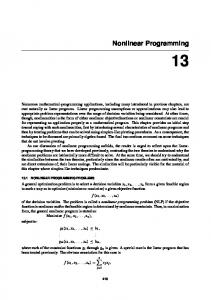
Thus y2 is the reduced set of (n — m) unconstrained variables, and y i is the vector of residuals of the linear constraint equations, which must of course be zero if the constraints are satisfied. Equations (5.2.4) represent a one-to-one transformation from x-space to y-space, which can be written in matrix form : lbl rYil = [Ai r A2 T1 [x i l I J Lx2 ] 10 j L 0 LY2] (5.2.5)

with its inverse transformation: rx,1 Lx2_1

1. (A 1 -1 )T — (A2A1-1)T1 [l

L

1

0

] LY2J

r(A1 -1 )T bl j• 0 L

The transformation is illustrated for two variables and one constraint in Fig. 5.1a.

FIG.

5.1a.

Clearly this is only one possible transformation to a set of co-ordinates y where the subset y, measures departure from the constraints and the subset y 2 measures position within the constraint space. More generally we may use a transformation of the form y, = U(A Tx — b), y2

= VTx — v,

(5.2.6)

152

R. W. H. SARGENT

which for convenience we shall write as y = Tx — d, with

x = T -1 (y + d),

= [AUT V] .

(5.2.7)

Here, y i = 0 if and only if the constraints are satisfied, provided that U is a non-singular m x m matrix. We also require y 2 to span the constraint space, and this will be so if the columns of A and V together span the whole space. Within these restrictions many choices of U and V are possible, and we shall naturally seek choices which make it easy to obtain the inverse transformation. A particularly simple inversion is obtained if we choose U and V so that the y-co-ordinates form an orthonormal system. We then have

TTT = I, and it follows that ATV = 0,

UTU = (ATA) x = TT(y + d).

V TV = I, VV T = I — A(ATA) - I AT,

(5.2.8)

This transformation is illustrated in Fig. 5.1b. For n > 2 it is not uniquely specified by (5.2.8), but we shall see later that it is not necessary to make a specific choice for the purpose in hand. X2

FIG.

5.1b.

To solve the minimization problem we are interested in the properties of the mapping of the objective function from x-space into y-space: F(x) —f(y). For this section we shall denote the corresponding gradients by VF and Vf; where it is understood that the differential operator V is in the

REDUCED-GRADIENT AND PROJECTION METHODS

153

appropriate co-ordinates; we also partition VF and Vf to conform with the partitions of x and y

VF

VIF1

Vf =I_

V2F

V , fl V2 f j

By the chain rule we have

OF vn Of ay, Oxj = = i ay, axj ' and hence, using (5.2.7):

VF = TTVf = A UT V l f + VV2f.

(5.2.9)

Now to solve the constrained minimization problem (5.2.2) we set y i = 0 and seek a stationary point of f(y) with respect to the y 2-co-ordinates, obtaining V2f = 0. Thus from (5.2.9) it follows that VF(R) = Ak, = UT Vif()

where

(5.2.10)

J

and St, are the co-ordinates of the point which solves problem (5.2.2). We recognize k as the vector of Lagrange multipliers for this problem, and from (5.2.10) we can obtain a very simple interpretation of their significance. For this purpose let us define c = ATx — b, so that from (5.2.6) we have y, = Uc, and consider the mapping f(y„ y 2 ) cgc, The chain rule gives

a(1) aci

=

N

ayi

ayi aci (5.2.11)

which can be written as V i O = UT V i f + V, f,

but at the constrained minimum c = 0, y2 = S'2 and V2f = 0, so from (5.2.10) and (5.2.11) we have (5.2.12) = VICO, 52). Thus I, measures the rate of change of the minimum value of the objective function as the constraint residuals change from zero. It is this property of Lagrange multipliers which make them useful in determining whether to leave a constraint in inequality constrained problems. Most unconstrained minimization algorithms make use of gradients, which means that we shall require values of V2f. However the computer subroutine provides VF for given values of x, so that for each gradient evaluation we need to transform from y to x variables, evaluate VF, then transform this

154

R. W. H. SARGENT

back to Vf. Often it will be more efficient not to introduce the y-co-ordinates explicitly, but to find expressions for the vectors required in terms of the x-co-ordinates. Thus a step sy in the constraint space coinciding with V2 f is given by

0 1_l0 0]

= [Sy 1 ] =[ '

[OY 2]

[V 2f]

1_0 I •

Vf

•

Using (5.2.7) and (5.2.9) the image of Sy in x-space, known as the "reduced gradient" is given by g(x) = T -14 =

[

00 ] (T') T VF(x). 0 I

(5.2.13)

Similarly, from (5.2.9) and (5.2.10) we obtain the expression for the Lagrange multipliers: (5.2.14) = [UT 0] Vf($t) = [U T 0] (T -1 ) T VF(). The reduced gradient lies in the constraint space, so if we start with a point x"" satisfying the constraints and use successive values of g R(k) as gradients in an unconstrained minimization algorithm, all points x satisfy the constraints, and if the algorithm is successful they will converge to the constrained minimum t. Equation (5.2.14) then provides the Lagrange multipliers if these are required. An initial feasible point is easily obtained by choosing any vector y, with y = 0 and carrying out the inverse transformation in (5.2.7). The original reduced-gradient method, due to Wolfe (1967), used the simple variable-elimination method described by (5.2.5). In this system we have from (5.2.5), (5.2.13) and (5.2.14): 9R(x) = [(A

2A, (A2A1 _1) A1 i ) T (A2

— (A2A1 -1 )

VF(x),

(5.2.15)

= [A, -1- 0] VF(x). For the orthonormal transformation given by (5.2.8) we have g(x) = (I — A(A TA) -1 AT) VF(x),

(5.2.16)

= (A TA) -1 AT VF(x). In this case the reduced gradient is simply the orthogonal projection of the gradient VF onto the constraint space. It will be seen that the expressions in (5.2.16) merely involve A and do not depend on the explicit choice of U and V, as indicated previously. It should be noted that the reduced gradient is a vector-valued function of position, since it depends on the gradient VF(x). However the matrix which

REDUCED-GRADIENT AND PROJECTION METHODS

155

transforms VF(x) to g(x) depends only on the constraint gradients (and the arbitrary matrices U and V), and is therefore a fixed constant matrix if the constraints are linear. The concept of the reduced gradient can still be used if the constraints are nonlinear by modifying the transformation to • yi = Uc(x), (5.2.17) Y2 = V T X — V. j

All the relations concerning gradients and Lagrange multipliers then remain unchanged, except of course that the matrix A must be evaluated at the current x. The reduced gradient now lies in the tangent hyperplane to the constraint manifold, so that any finite step along it will in general leave the manifold. To deal with this problem Arrow, Hurwicz and Uzawa (1958) proposed a continuous steepest-descent method based on integrating the system of differential equations: dx (5.2.18) x(0) = x 0, = —9(x), where xo is an initial feasible point. It should be noted that since the transformation is now nonlinear, finding an initial feasible point is no longer a trivial matter. Of course (5.2.17) must usually be integrated numerically, and since we are not interested in the whole trajectory but only its limit point, stability is a more important consideration than accuracy. Standard explicit methods, such as the Runge—Kutta methods would normally require prohibitively small steplengths, and the best choice would seem to be a low order predictor-corrector method. Arrow, Hurwicz and Uzawa do not discuss the practical implementation of their algorithm, but Branin and Hoo (1972) report some success with a similar approach to unconstrained problems, extending the idea to a continuous version of Newton and quasi-Newton methods. A more direct approach is to make an initial step along the reducedgradient direction and then use a Newton-type correction procedure to return to a point satisfying the nonlinear constraints, according to the scheme: for r = 0: for r

1:

s(k,O) =

x(k+1.1)

x(k) =

T(x(k+ ) s(k,r) = — [

S(k,r) = X(k+ 1 r+ 1) — X (k +1 • where The essential idea is illustrated in Fig. 5.2.

cx (k)

g (x(k)) ;

UC(X(k i 'r))1

0

(5.2.19)

156

R. W. H. SARGENT

Constraint

FIG. 5.2.

For the variable-elimination method the correction formula reduces to A1(X(1+1 "))

(k") = — C(x k+ l 'r)) ;

S2(" = 0,

(5.2.20)

while for the orthonormal transformation we obtain Sa'r) =

A(ATA) -1 c(x(k L'))

(5.2.21)

where obviously A is evaluated at 0-1-1'). In fact it is hardly worth re-evaluating the gradients for each iteration of the correction procedure, for the constituent matrices for the correction must be evaluated at x order to compute 9R (x) and can then be used systematically at each iteration of the correction. Although this simplified Newton procedure has only linear convergence, the saving per iteration is more than enough to justify its use. In fact Abadie and Carpentier (1969), who applied this technique in conjunction with the variable-elimination method, suggest an approximate correction to the stored value of AT 1 , according to the formula: A 1-1(yek +1,)

) 2A I-1 (e)) — A r (x(k))Ai (x(k+ L')) A Zi (x(k)). (5.2.22)

However, if one is going to re-evaluate A 1 it would seem preferable to recompute its triangular factors rather than use this approximation. It is well known that the steepest-descent method is inefficient, but a similar technique can be used in conjunction with other methods. With linear constraints any conjugate-direction or quasi-Newton method using the reduced gradients will generate a search direction p (k) lying in the constraint manifold. For nonlinear constraints the curvature prevents the successive vectors from lying in a linear manifold, but a similarly constructed search direction will be close to the tangent hyperplane if the curvature is not too great, and in any case the iterative correction procedure will correct for this additional inherited effect of the constraint curvature. Abadie and Carpentier

REDUCED-GRADIENT AND PROJECTION METHODS

157

(1969) in fact incorporated the Fletcher—Reeves conjugate-gradient procedure in one version of their "generalized reduced gradient" (GRG) procedure, referred to above. Finally we note that the correction procedure can be used to find an initial feasible point, although convergence can be proved only for a sufficiently good initial guess, as is usual for Newton-type procedures. On succeeding iterations the distance of the initial point e+ 1 1 ) from the constraint manifold can be controlled by reducing 2(k) and hence this can always be chosen small enough to ensure convergence of the correction procedure. Projection Methods

A solution ft of the equality constrained problem (5.2.1) corresponds to a stationary point of its Lagrangian function: L(x, ).) = F(x) — Tc(x).

(5.2.23)

Thus we have g(52) — A(k)1, = 0,

(5.2.24)

c(ft) = 0.

This system of nonlinear equations could be solved by standard techniques, but it is better to construct methods which take account of the special structure of the system. We wish to make local approximations to the functions about a current point x, so we consider the problem of finding the step s from this point which attains the feasible point with the lowest value of the objective function within a distance (5 from x:

min {F(x + s) : c(x + s) = 0,

sTs < 62 ).

(5.2.25)

If this problem has a solution this must satisfy the conditions: g(x + s) — A(x + s) + ps = 0, 1 c(x + = 0. f

(5.2.26)

The Kuhn—Tucker multiplier p is either zero, in which case the step-size constraint has not affected the problem, or kt > 0 and 11s11 = 6. We now choose 6 small enough to justify replacing the nonlinear constraints by their second-order Taylor expansions: F(x + s) = F(x) + eg(x) + isTG(x) s, ci(x + s) = ci(x) + sTai(x) + isTGi(x) s,

j =

1, 2, . . . , fl

} (5.2.27)

158

R. W. H. SARGENT

Differentiating and substituting the result in the first equation of (5.2.26) gives j(x) + G(x)s) + ps = 0.

(x) + G(x) s) —

(5.2.28)

1=1

If we write W(x) = G(x) —

Aj G(x)

and W(x) = W(x) + pI,

this can be rearranged to give W(x) s = A(x) A — g(x),

(5.2.29)

c(x + s) = 0. Choice of a value of !L > 0 implicitly fixes the step size 6 = Ils11, and the larger the value of kI, the smaller the step size. It is interesting to note however that in principle the system (5.2.29) has a solution (s, A) for any chosen p, so this indirect method of fixing 6 ensures that the constraint set is always attainable, no matter how far x is from this set. Thus, to be sure of the validity of our second-order approximation, x must be close to the constraint manifold. System (5.2.29) is somewhat simpler to solve than system (5.2.26) since its first equation is linear in s for given p and A, but we still have to choose A so that the resulting s satisfies the nonlinear constraint equations, and the quadratic approximation to the constraints makes no essential simplification here. However if 6 is small enough to justify a linear approximation to the constraints, this difficulty disappears and we obtain a set of linear equations to determine A. By substituting for s from the first equation of (5.2.29) into this linear approximation we obtain the system: Ws=Ak—g,

(5.2.30)

(ArW - 'A) = ATW - ig — c,

where it is understood that c, A, g, W are all evaluated at x. To be consistent we should also neglect the second-order constraint terms in W, which would then give the system: Cs=AX—g,

1

(ATG -1 A) = ATG - 'g — c, j

(5.2.31)

where we have written G = G(x) + pi. If the constraints are in fact linear, equations (5.2.31) provide a Newton-type procedure for solving the problem. The first step gives a point satisfying the constraints, and the remaining steps are similar to an unconstrained Newton

REDUCED-GRADIENT AND PROJECTION METHODS

159

procedure within the constraint space. Convergence is assured for a sufficiently large value of p, and this unconstrained procedure is recognizable as the well known Levenberg-Marquardt algorithm, first proposed for use in unconstrained least-squares problems by Levenberg (1944). As p becomes large, pI and W pI, and equations (5.2.30) and (5.2.31) both tend to the form s = p -1 (AX - g) 1 p

(ATA) = p 'A Tg - c.

(5.2.32)

When the point x satisfies the constraints we have c = 0 and (5.2.32) then gives X = (ATA)"Arg, s = - p' {I - A(ATA)'AT} g.

(5.2.33)

Comparison of (5.2.33) with (5.2.16) shows that this first-order approximation for the constrained steepest-descent direction s is just the orthogonal projection of the objective function gradient onto the constraint space. Putting c = 0 in (5.2.30) or (5.2.31) produces a similar kind of formula; for example, (5.2.30) gives = (ATW -1A) -1ATW - lg, s = {I - W"A(A TW'A) -1 AT } W -19.

(5.2.34)

This is also a projection onto the constraint space, for it is easily verified that any component of g orthogonal to the constraint space (of form Az) is annihilated by the matrix operator. Indeed, if we transform to a new system of co-ordinates: y = Wx, with corresponding transformations of c, A, g, s, equations (5.2.34) reduce to the form (5.2.33) in the new co-ordinates. Since the metric W - * of this transformation depends on the point x, it is reasonable to call projections of the type defined by (5.2.30) and (5.2.31) "variable-metric" projections. Although these formulae have been developed in terms of the true Hessian matrices of the various functions, and are indeed usable in this form, they are more often used with approximations to these matrices, obtained by quasiNewton techniques. In particular, equations (5.2.30) involving W(x) would normally make prohibitive demands on storage, if not computation time, if all the G(x) matrices had to be separately evaluated. However it is easy to generate a quasi-Newton approximation to W itself, for we note that it is the Hessian matrix of the Lagrangian function (5.2.23), whose gradient is simply (g - AX).

160

R. W. H. SARGENT

The use of the Levenberg-Marquardt rule is not the only means of limiting the step size. The basic objective is to choose a step size such that the Lagrangian function (5.2.23) is well approximated by terms up to second order, and we might equally well choose s to make the second-order terms themselves suitably small, by requiring that is T W(x) s < 62 . The analogue of (5.2.28) is then (g (x) + G(x) s) —

(ai(X)

G(x) s) 2; + pWs = 0,

(5.2.35)

leading to the system Ws = oc(AA. — g),

(5.2.36)

c(x + s) = 0,

where we have written a = 1/(1 + 1.0 , so that 0 < a < 1, and the step-size decreases from its unconstrained value as a decreases from unity. The version analogous to (5.2.30), corresponding to linearizing the constraints, is then W s = a(Ak — g), a(A.TW -1A) = aATW - — c.

•

(5.2.37)

It is of some interest to compare these two alternative methods of limiting the step size by comparing (5.2.30) and (5.2.37). Of course for t = 0 and a = 1 both formulae give the same result: a variable-metric projection of x onto the constraint manifold plus a variable-metric projection of the gradient g. For (5.2.37), as a decreases from unity the only effect is to scale down the distance travelled in the constraint space along the projected gradient, as shown in Fig. 5.3a. For (5.2.30) on the other hand, as p increases from zero both projections rotate towards the orthogonal projections, also producing a decrease in step-size, as shown in Fig. 5.3b. In one sense system (5.2.37) may seem more logical, for the step size is measured in the same metric as appears in the projection, but in fact this interpretation only makes sense if W is positive definite. It must of course be non-singular for the inverse W -1 to exist, but if it is not also positive definite we are not assured of obtaining a decrease in the objective function for sufficiently small a. In contrast, W is always positive definite for sufficiently large /.2, so there are no difficulties about inverses and descent steps. For Newton-type methods, which actually evaluate G, and if necessary the Gi, for use in the formulae, there is thus an over-riding advantage in using the Levenberg-Marquardt rule. However, if a quasi-Newton method is used to approximate G or W it is possible to use a scheme which ensures that the approximation remains positive-definite. Of course, if the true matrix is not -

REDUCED-GRADIENT AND PROJECTION METHODS

(i) Projection into constraint

FIG.

5.3a.

161

162

R. W. H. SARGENT

( i ) Projection into constraint

sr s

( ii) Projection in constraint — plane

Flo. 5.3b.

163

REDUCED-GRADIENT AND PROJECTION METHODS

positive-definite, such an approximating scheme is imposing an artificial modification very similar to that imposed by the Levenberg-Marquardt rule, and there is no theoretical basis for choosing between them. Some quasiNewton methods require minimization of the objective function along the successive search directions, and this provides a quite different reason for choosing system (5.2.36) or its analogues. However, to secure convergence of any of the schemes a simple decrease of the function at each step is not sufficient, and it is necessary to impose a stronger "stability condition" of the type: F(k) _ F(k+ 1) o'er suol, (5.2.38) 0 < ö < 1. From the above discussion it is where sm = x(k + 1) x clear that this can always be satisfied with a suitably small step provided that the underlying matrix is positive definite. Both conditions are achieved using a single parameter, g, in the Levenberg-Marquardt scheme, while the use of a to control step size requires separate attention to the problem of maintaining positive definiteness of the matrix. We now have complete schemes for dealing with linearly constrained problems, based on either (5.2.31) or the analogue of (5.2.37) (with W replaced by G). However for nonlinear constraints these schemes replace the curved constraint manifold by its tangent hyperplane, and as for the reduced gradient methods we have the problem of following the curved constraint. In effect this means returning to the schemes (5.2.29) or (5.2.36), but we can again use the linearized schemes, (5.2.30) and (5.2.37) respectively, as the basis for a Newton-type correction procedure. For the solution of (5.2.36), where x = x s = soo, the scheme used is: ,

for r = 0: cx (k)(Arw

- 1A) k(k,0) = oc(k)ATw - 'g w s(k,O) = 01(k)(Ak(k,O)

/el' 1.1) = x(k) for r

c(x(k)),

g),

s(") ; •

1:

(5.2.39)

(k) (Arw - I A) okoc.0 = _ c (x(k + 1,1)) , 6s(k4 =

x (k + 1,r + 1)

x(k +1,r) + o s(k,r) ,

+ 1) = 1, (k,r)

ok(k,r) . •

It suffices to use a simplified Newton scheme, in which g, A, W in (5.2.39) are all evaluated at the point x (k) . The analogous scheme for solving (5.2.29) is obtained from (5.2.39) by setting au') = 1 and replacing W by W.

R. W. H. SARGENT 164 If the correction procedure converges (within say 10 iterations), we set x(k +1) = e+14 and soo=x(k+i)-x00 and test the stability condition (5.2.38). If this is not satisfied, or if the correction procedure does not converge, the whole step is repeated with a smaller value of a(k) (or a larger value of gm). As with the reduced-gradient methods, the correction procedure can also be used to obtain an initial feasible point. Since the correction procedure is iterative, one must set a tolerance for the convergence and this can be either on the step size ps(k.o. < a, or on the residual lic(x("'"))11 < a, or indeed one can insist on both. It can be argued that there is little point in iterating to high accuracy on this correction when far from the solution, and hence that one should start with a relatively large a in the test and reduce this as the constrained minimum is approached. Unfortunately there are hidden pitfalls in this idea, for proof of convergence relies on the generation of a sequence of descent steps in a compact space, achieved by satisfying the stability condition (5.2.38) at each step. If at any time a violation of the constraints larger than the final acceptable tolerance is allowed, it is possible to find a point where the objective function has a lower value than at any feasible point, and then condition (5.2.38) actually prevents recovery to an acceptable point. What one would like to do is to allow an increase in the objective function if this results in a decrease in the constraint violation, and one way of achieving this is to add a penalty term to the objective function if the constraints are violated; for example one could replace F(x) by the penalty function:

P(x, r) = F (x) r c (x) T c (x)]

(5.2.40)

By making r sufficiently large we can make the minimum of P(x, r) arbitrarily close to the constrained minimum of F(x), and hence use an unconstrained minimization technique applied to P(x,r); such methods will be discussed by Ryan. However, we know that the Lagrangian has a stationary point at the constrained minimum, and much smaller values of r ensure that this stationary point is in fact a minimum. Thus if the step size is chosen to satisfy the stability condition (5.2.38) applied to the Lagrangian of P(x, r), the so-called "augmented Lagrangian function", this will force convergence without the need to insist on feasibility at each step. This is the idea behind the "augmented Lagrangian" methods to be described by Fletcher, and also his "exact penalty function" method. Unfortunately, although there is a finite threshold value of r to achieve this result, there is no a priori way of obtaining a suitable lower bound for it— it clearly depends on the curvature of the objective and constraint functions at the solution. Nevertheless, even if we do not rely completely on the penalty term to satisfy the constraints, it may still be useful to replace F(x) by P(x, r) if the constraints are strongly curved, for then the initial projection step will

REDUCED-GRADIENT AND PROJECTION METHODS

165

not cause such a strong violation of the constraints and less work will be required in the correction procedure. This device should not be so necessary with the projections employing W since this already incorporates constraint curvature information. In conclusion, it should be pointed out that the distinction between reduced-gradient and projection methods is artificial, for although the motivating ideas may seem different both approaches lead to methods of the same type. Indeed any given method can be derived using either approach, as we have shown in the case of the orthogonal-projection method. In both cases the step at each iteration is a projection of the current point into the constraint manifold, combined with a similar projection of the objective function gradient. The essence of the choice between methods is the choice of metric for the projection, and this point will be taken up again after considering inequality constraints. 5.3. Inequality Constraints—Active Set Strategies Most strategies for solving a linear inequality-constrained problem start with a feasible point, seek a feasible search direction from this point, then move along this direction until either the objective function passes through a minimum or a new constraint is encountered; the process is repeated from this new point. A simple illustration is given in Fig. 5.4. One method of finding a feasible direction from a given point x(k) is to find the set of constraints satisfied as equalities at x(k) and project the objective this set. If the projection gives a non-zero step this function gradient g defines a feasible direction; if not we are at a stationary point in the constraint space and the Lagrange multipliers can be used to test if we can decrease the objective function by leaving any of the constraints. If the constraints are of the form A ra( b, equation (5.2.12) shows that this will be so for any constraint corresponding to a negative A i, and since A; is the rate of change of the objective function it is logical to drop the constraint with the most negative Al. We then repeat the process with the reduced set of constraints, continuing until either a non-zero projection is obtained, or all A; are positive. The latter condition indicates that X (k) is a Kuhn–Tucker point and the algorithm is terminated. The set of constraints treated as equalities in determining the feasible direction is called the active set of constraints at point x(k) . As Powell has pointed out in Chapter I, such an algorithm must converge since constraints are not dropped from the active set unless a stationary point has been attained in this set, and since the next step reduces the objective function value below its value at this point, one cannot return to it. The objective function will normally have only a finite number of stationary points with

166

R. W. H. SARGENT

distinct values in each active set, and the total number of possible active sets is finite, so the process must terminate.

FIG. 5.4.

We note that the active set need not be constituted afresh at each iteration, since the search direction lies in the current active set and all constraints in it will therefore be satisfied as equalities at the new point; there will only be an addition to this if the step along the search direction encounters a new constraint. The idea of minimizing the objective function along the search direction derives from the use of steepest-descent or quasiNewton methods which require this, but it is of course not an essential feature; the step can be of the length prescribed by the projection algorithm used unless this is truncated by encountering a new constraint. For nonlinear constraints, the basic projection step before correction will normally give a non-feasible point, so one must include the correction iterations as part of the step. There then arises the problem that one or more new constraints may be encountered before the correction procedure converges, and hence while the point is still infeasible. Rosen (1961), who first proposed active set strategies for nonlinear-programming problems in

REDUCED-GRADIENT AND PROJECTION METHODS

167

connection with the orthogonal gradient-projection procedure, (cf. equations (5.2.33)), suggested reducing cek) (= p -1) until the final corrected step came within the desired tolerance of the nearest newly-encountered constraint, as shown in Fig. 5.5. However this process would seem to require iteration on ay') and it is better to add the new constraint to the active set as soon as it is violated, so that the correction procedure itself obtains the required solution; indeed one can also treat any further violated constraints in the same way. It is just possible to obtain n constraints in the active set in this process, which of course have a unique point of intersection so that the projected correction step is zero; only in such a case will it then be necessary to reduce ay') (or p(k) in the relevant algorithms) to obtain successful correction to a feasible point. Abadie and Carpentier (1969) use this strategy in their generalized reduced-gradient method, and so do Sargent and Murtagh (1973) in their variable-metric projection method based on equations (5.2.34).

Sargent and Murtagh (1973) also use slightly different rules for adding a constraint, which are illustrated in Fig. 5.6. For any point x (whether at the start of an iteration or during the correction procedure) a projection step s is computed for the current active set. If the new point (x + s) is feasible with respect to inactive constraints, as in Figs 5.6a or 5.6b, the step is made without changing the active set. If on the other hand a new constraint j is violated at (x + s) the action depends on e j(x). If Ilei(x)11 is larger than a specified tolerance the new point is x + ccs, where cc is chosen so that the point is on the linearization of cj (x) about x(k) ; otherwise constraint j is added to the active set and the projection step recomputed. If several new constraints

168

R. W. H. SARGENT

are violated the nearest constraint (that is the one with the smallest value of a) is selected. This rule avoids computing intersection points of search directions with nonlinear constraints, and occasionally saves needless addition of constraints to the active set.

x,

(b)

x,

Id) FIG. 5.6.

Rosen (1961) in fact did not drop the constraint with the most negative Lagrange multiplier, but used instead a first-order estimate of the change in objective function due to the change in projected step when the constraint is dropped. The variable-metric analogue of this formula c.f. Sargent and Murtagh (1973), corresponding to (5.2.37) is AF; g(k) 'As; = 2 i2 /mE,

( 5.3.1)

REDUCED-GRADIENT AND PROJECTION METHODS

169

where As is the change in step due to dropping constraint j from the active set and AFJ is the corresponding change in the objective function; A; is the Lagrange multiplier, as given by (5.3.37), and ini; is the corresponding diagonal element of the matrix (A rW -1A) - ` . Rosen's formula is of course obtained by setting W = I. Thus the constraint to be dropped is the one among those with negative which has the largest value of (Alim ij); we note in this connection that rnii > 0 if W is positive definite and the active constraints are linearly independent. This appears to be a better criterion, and since it is valid for every x can be used to test whether it is advantageous to drop a constraint at every iteration, rather than waiting until a stationary point is attained in the current set. We can even use it to drop all but the minimum active set required to obtain a feasible direction. Note that dropping a constraint changes the projection, and hence the magnitudes, and perhaps also the signs, of the Aj for the remaining constraints; thus the constraints must be dropped one at a time, recomputing the ).; each time, until no negative A i remain. Several authors have used such a strategy, and Sargent and Murtagh (1973) in their algorithm test for dropping constraints in this way every time a constraint is added to the active set, whether this is in the basic step of the iteration or during the correction procedure. This further decreases the chances of building up a set of n active constraints and makes the best possible step at every stage. Again Powell has pointed out that "zigzagging" can occur when constraints are dropped before waiting to attain a constrained stationary point, and that this may slow down convergence or even prevent it. Various ad hoc devices have been suggested for dealing with zigzagging, but the only "anti-zigzagging rule" which enables one to prove convergence is the one proposed by Zoutendijk (1960): "If a constraint previously dropped from an active set is added again, it is retained in the active set until a constrained stationary point is attained". In fact it seems that variable-metric projection algorithms are much less prone to zigzagging, and although the Zoutendijk rule is incorporated in our algorithm (Sargent and Murtagh, 1973) it seems to be rarely activated. The combination of active set selection and projection is in effect attempting to solve the problem: W s = cc(AX. g), c(x + s) 0, A.

0,

(5.3.2)

where W, A, g are all evaluated at x = e), a = am is fixed, and A here represents the complete set of constraints. We note that since all cf(x + s)

170

R. W. II. SARGENT

and 2; must be non-negative, the final equation in (5.3.2), known as the complementarity condition, ensures that i ci(x + s) = 0 for each j = 1, 2, ..., m, so that 2.1 and ci(x + s) cannot both be non-zero at the same time; a non-zero ki indicates that constraint j is active at the solution of (5.3.2). By making a local linear approximation to the constraint functions, we can develop a simplified Newton procedure to solve (5.3.2), by solving the sequence of problems: — x(k)) = a(A)"L") — g) 4) (k + 1,r) = c(k + 1,• 1) + AT(x(k +1,r) x (k + - 1)) (5.3.3) (k+ 1.r) 4) (k + 1,r) ?...„ 05 0, -

[k(k + 1,1T[4)(k + 10)] = 0 ,

for r 1, where x(k+1.°) = x(k). This is exactly equivalent to solving the sequence of quadratic programming problems: min {ag Ts + 4-sTWs} subject to

(5.3.4) = [c(k+

i) — AT(X(k l 'r 1) —

3L(k) )]

ATS 0,

= x00 ± s.

The Sargent and Murtagh (1973) strategy usually achieves the solution of (5.3.2) via (5.3.3). However it fails to do so if the procedure stops at an infeasible point because the active set has built up to n constraints, and the solution then has to be restarted with a smaller value of a. Also, as with all active set strategies considered so far, it requires an initial feasible point for convergence to be guaranteed, and for nonlinear constraints the finding of such a point is not a trivial problem. It is possible to add further refinements to deal with both of these problems, but the resulting algorithm becomes rather cumbersome and a simpler, more direct approach is available, as described by Sargent (1973). In this approach we first eliminate x(k+1 ,0 from (5.3.3) to yield a "linear complementarity problem": } = q + MX, (5.3.5) X ?, 0, 0, X7 4) = 0, where we have written q

ek+10.- 1)

x(k+ 1,r),

M

AT(x(k + 1,r - 1)

x (k)

=

I A, - 19).

(5.3.6)

REDUCED-GRADIENT AND PROJECTION METHODS

171

From the form (5.3.4) we know that there exists a unique solution to the problem provided that the constraints are consistent, and it can be shown that this will be so for all r provided that they are consistent at x a is chosen sufficiently small. Further, there is an algorithm due to Lemke (1968) which provides a straightforward procedure for finding this solution or demonstrating that no solution exists. Q

FIG. 5.7.

Thus the strategy is to start with an arbitrary a (e.g. a = I) and use the Lemke algorithm to solve the sequence of problems (5.3.3) until the convergence criterion is satisfied. If no solution is indicated at any stage, the process is repeated with a smaller value of a. The Lemke algorithm for solving (5.3.5) adds a slack vector: (t) = + moA0 + (t•

0,

where usually m oT = [1, 1, ...

0,

20

0,

(5.3.7)

172

k. W. If. SARGENT

We start with 1. = 0, .1 0 = 0, and then increase A o until we just have 0. At this point we have 0.1 = 0 for some constraint j, so the appropriate value of 1 0 is obtained by solving the jth equation for ,1 0 ; this is achieved by the pivot operation of linear programming, putting A o on the left-hand side of the jth equation and O f on the right-hand side. Since ck i = 0 we can now increase Al from zero without violating the "complementarity condition" kr+ = 0. Thus we increase ki until some Ok is just reduced to zero. We again pivot, solving the kth equation for 21, and can then repeat the process with ilk This "complementary pivoting" procedure is repeated until eventually it is .1.0 which is just reduced to zero, with all other left-hand side variables still positive. This of course gives a solution to the original problem (5.3.5). Full details will be found in Lemke's paper, where a proof of finite termination for the quadratic programming problem is also given. feasible the sequence of Sargent (1973) has shown that if x correction steps in (5.3.3) converges to the solution of (5.3.2) for sufficiently small a(k) , and that the primary sequence of solutions to (5.3.2) converges to a Kuhn—Tucker point of the full nonlinear programming problem provided that au') is also chosen small enough to satisfy the stability condition (5.2.38) for each k. In most cases the procedure will in fact converge from an initial infeasible point, but of course the stability condition must not be used until a feasible point is attained. In case of difficulty, convergence can be forced by replacing F(x) by the penalty function P(x, r) of equation (5.2.40) with suitably large r, in which case the stability condition is applied from the beginning. Alternatively, to avoid the need for estimating r, a feasible point can be found by applying the standard algorithm, including the stability condition, with the objective function k(x) Tc(x)]. It is not in fact necessary for the convergence proof to solve each quadratic program completely. A partial solution of (5.3.5), with everything satisfied except for some of the non-negativity conditions on the Ai, corresponds to a feasible solution with some constraints held as equalities. Such a solution suffices, provided that these constraints are held as equalities in the remaining iterations of the current correction cycle. This is simply achieved in the Lemke algorithm by first pivoting the corresponding A i to the left-hand side, and then ignoring them. Any equality constraints in the original problem are dealt with similarly. In all the equations developed in the paper the implicit assumption has been made that inverses of matrices exist wherever they are required. This is ensured by making a "non-degeneracy assumption" for the constraints, which requires that for every point x, every set of n gradient vectors ai(x) is a linearly independent set. For linear constraints, any degeneracy among them can be eliminated at the outset by making small perturbations of the original

REDUCED-GRADIENT AND PROJECTION METHODS

173

set, as is done in linear programming. For nonlinear constraints there is a chance that an active set of linear approximations becomes degenerate, but since the gradients are a function of x this situation will normally be resolved by changing the step, for example by reducing GO ) . In the algorithms described, all that is necessary is to use a test for linear dependence before adding a constraint in order to take the appropriate action. It is perhaps worth adding a final comment on the use of slack variables. In linear programming all general inequality constraints are converted to equalities by the addition of slack variables, so that the only inequalities left in the problem are non-negativity conditions on the extended set of variables. This technique was adopted by Wolfe (1967) in his reducedgradient method, and also by Abadie and Carpentier (1969) in their extension of this method to deal with nonlinear constraints. Sargent and Murtagh (1973) dealt with linear inequalities as such, but advocated the use of slack variables for converting nonlinear constraints to equalities. They point out that, since slack variables appear only linearly, the Hessian matrices G and W have null rows and columns which may cause difficulties unless special precautions are taken to maintain positive-definiteness of their approximations. Since, as we have seen, it is perfectly possible to deal with linear and nonlinear inequalities directly, there appears to be no good reason for enlarging the problem and adding extra complications by using slack variables. 5.4. Summary

The ingredients of a nonlinear programming algorithm are as follows. 1. An active set strategy for selecting a set of constraints to be treated as equalities in the current step. 2. A projection formula for predicting a step in the active set. 3. Formulae for updating the matrices associated with the projection formula. 4. A correction procedure to follow nonlinear constraints. 5. A stability test to ensure convergence. It will be clear from the discussion that I favour an active set strategy which does not rely on an initial feasible point. The use of the Lemke algorithm effectively combines the active set strategy with the projection formula, but there is not as yet sufficient experience to judge whether it is better to solve the quadratic program completely at each step or not. The simplest correction procedure is the simplified Newton method, which does not require re-evaluation of gradients during the correction. Its operation may be aided by adding a penalty term to the objective function.

174

R. W. H. SARGENT

There is no real distinction between reduced-gradient and projection methods. All methods require storage of a transformation matrix or projection matrix of some sort, and the quasi-Newton methods require in addition the storage of a Hessian matrix approximation. For very large problems there may therefore be some merit in using a reduced-gradient (elimination of variables) or orthogonal projection, combined with a conjugate-gradient algorithm, as in Abadie's GRG method. Otherwise there is every advantage in using the variable-metric projection methods based on a quasi-Newton approximation to W or W, storing the matrices W and ATW - i A or their equivalents. Clearly one would store and update triangular factors rather than inverses.

27.

1.

Wolfe, P.,

"Methods for Nonlinear Constraints" in J. Abadie (Ed.),

"Nonlinear Programming", pp.120-131, North Holland Publishing Co. (Amsterdam, 1967).

2.

Arrow, K.J., Hurwicz, L., and Uzawa, H.,

"Studies in Linear and Nonlinear

Programming", Stanford University Press (Stanford, 1958).

3.

Branin, F.H. and Hoo, S.K.,

"A Method for finding Multiple Extrema of a

Function of n Variables" in P.A. Lootsma (Ed.) "Numerical Methods for Nonlinear Optimization", pp.231-237, Academic Press (London, 1972).

4.

Abadie, J., and Carpentier, J.,

"Generalization of the Wolfe Reduced

Gradient Method to the Case of Nonlinear Constraints", in R. Fletcher (Ed.) "Optimization", pp.37-49, Academic Press, (London, 1969).

5.

Levenberg, K.,

"A Method for the Solution of Certain Nonlinear Problems in

Least-Squares", Q. Appl. Math. 2, 164-168, (1944).

6.

Rosen, J.B.,

"The Gradient Projection Method for Nonlinear Programming"

Journal Soc. Ind. Appl. Math.: "Part I - Linear Constraints" 8 181-217 (1960), "Part II - Nonlinear Constraints" 9 514-532 (1961).

7.

Sargent, R.W.H., and Murtagh, B.A.,

"Projection Methods for Nonlinear

Programming", presented at 7th Mathematical Programming Symposium, The Hague, September 1970 - published in Mathematical Programming 4, 245-268 (1973).

Murtagh, B.A., and Sargent, R.W.H.,

"A Constrained Minimization Method with

Quadratic Convergence" in R. Fletcher (Ed.) "Optimization", pp.215-246, Academic Press (London, 1969).

8.

Zoutendijk, G.,

9.

Lemke, C.E.,

"Methods of Feasible Directions", Elsevier (Amsterdam, 1960).

"On Complementary Pivot Theory" in G.B. Dantzig and

A.F. Veinott (Eds.) "Mathematics of the Decision Sciences, Part I" pp.95-114, American Mathematical Society (1968).

10.

Sargent, R.W.H., "Convergence Properties of Projection Methods for Nonlinear Programming" presented at 8th International Symposium on Mathematical Programming, Stanford, August 1973.