Dr Craig Roberts is a Lecturer at the School of Surveying and Spatial Information .... et al., 2003; Coughlin & Tung, 2004; Yu et al., 2005):. â Identify all extrema ...
Reducing Carrier Phase Errors with EMDWavelet for Precise GPS Positioning Jian Wang, School of Surveying and SIS, UNSW Jinling Wang, School of Surveying and SIS, UNSW Craig Roberts, School of Surveying and SIS, UNSW
BIOGRAPHY Dr Jian Wang is currently a Visiting Fellow at the School of Surveying & Spatial Information Systems, University of New South Wales (UNSW). He graduated with a PhD from the China University of Mining & Technology (CUMT) in 2006. His area of expertise is in the field of GNSS/INS integration with special emphasis on the quality control of navigation. He also focuses on the studies of wavelet theory for survey and geodetic applications. Dr Jinling Wang is a Senior Lecturer in the School of Surveying & Spatial Information Systems, UNSW. He is a member of the editorial board for the international journal GPS SOLUTIONS, and chairman of the international study group on pseudolite applications in positioning and navigation within the International Association of Geodesy's Commission 4. He was 2004 President of the International Association of Chinese Professionals in Global Positioning Systems (CPGPS). He holds a PhD in GPS/Geodesy from Curtin University of Technology, Australia. Dr Craig Roberts is a Lecturer at the School of Surveying and Spatial Information Systems, UNSW. He has worked as a private surveyor, as a geodetic engineer at UNAVCO, USA, and at the GeoForschungsZentrum, Germany, and lectured at RMIT University, Melbourne. His current research interests are leveraging CORS infrastructure for application to surveying and spatial information. ABSTRACT High precision GPS baseline calculation is feasible only when very precise carrier phase observations are available. Unfortunately these observations are often affected by systematic errors (such as multipath, ionospheric and tropospheric effects, orbit bias, etc). In this paper, a new EMD-Wavelet trend extraction model is
presented and integrated into a baseline calculation model for systematic error mitigation. The pre-divided frequency of the wavelet transform seriously affects its ability to extract trends of an input signal. The Empirical Mode Decomposition (EMD) technique is a new signal processing method for analysing non-linear time series, which decomposes a time series into a finite and often small number of Intrinsic Mode Functions (IMFs). The decomposition procedure is adaptive and data-driven. The IMFs are stationary, which are more suitable for wavelet analysis. Therefore the merits of both the EMD and Wavelets can be combined for systematic error extraction in double-difference (DD) carrier phase observables. Initial results from processing a simulated, mixed, nonlinear signal also shows the advantages and disadvantages of EMD and Wavelets respectively. These are used to produce an improved EMD-Wavelet trend extraction methodology using the following process. Firstly, the non-linear series are decomposed into stationary IMFs and residual components. Secondly, the selected high frequency IMFs are de-noised with the wavelet model, and, finally, the EMD reconstruction gives the extracted system error series. Signal-to-noise ratio (SNR) and root mean square error (RMSE) are used to quantitatively evaluate the trend extraction effect. Based on the proposed trend extraction model, the baseline resolution procedure is shown and experimental results demonstrate: z EMD-Wavelet model is more suitable for systematic error extraction. z High frequency IMFs are identified using Standardized Empirical Mean (SEM) of fine-to-coarse EMD reconstruction. z Baseline calculation stability and the DD residual series are greatly improved with the proposed procedure. The proposed systematic error extraction model can even be applied to baselines with more complicated system errors (eg when the atmosphere is affected by strong sunspot activity) and other applications requiring similar time series analysis.
INTRODUCTION Systematic errors are one of the most dominant factors inducing the failure of carrier phase-based high precision baseline solutions and their stability. There are many complicated factors causing systematic errors which are impossible to eliminate completely, including ionospheric and tropospheric errors, orbital errors, multipath and other unmodelled biases. Many methods have been employed to study the mitigation of the systematic errors for GPS baseline processing. Ionospheric and tropospheric error modelling has been intensively studies. Satirapod & Prapod (2005) investigated different tropospheric models and their effect on GPS baseline accuracy. Ionospheric error correction improvements of differential GPS for long baselines are presented in Mardian et al. (2003) and Hichem et al. (2006). The orbit bias is a baseline length dependent bias which can be minimized by Kalman filter modelling and carrier phase-difference modelling (Colombo et al, 1995; Han & Rizos, 1996). Multipath is another significant systematic error source. Finite impulse response (FIR) filters are tested with the limitation of dividing mixed multipath errors with the same frequency band (Han & Rizos, 1997; Satirapod & Rizos, 2005). Adaptive filter extraction and elimination of multipath is influenced by the difficulty in selecting the appropriate step-size parameter and the filter length, as investigated by Satirapod & Rizos (2005) and Ge et al. (2002). The effects of other unmodelled biases can also be mitigated to some extent with appropriate stochastic modelling. Wavelet noise reduction modelling is one of the most effective techniques for complex signal analysis. Recently it has been introduced into the field of GPS data processing for signal de-noising, outlier detection, bias separation and data compression (Satirapod & Rizos, 2005; Collin & Warnant, 1995; Ogaja et al., 2001), as well as models introducing wavelets for multipath analysis and mitigation for baseline solutions (Han & Rizos, 2000; Satirapod & Rizos, 2005; Ge et al., 2002). Although wavelet transforms are suitable for noise reduction - in other words, for signal trend extraction - its pre-divided frequency feature limits its ability to decompose the signal into different frequencies. Tthe inherent characteristics of Empirical Mode Decomposition (EMD) is a new signal analysis technique (Huang et al., 1998) showing great promise for signal trend extraction. EMD techniques have already been successfully applied to several other scientific problems (Yu et al., 2005). It provides an adaptive representation of non-linear signals, which ensures the non-linear signal can be converted into an Intrinsic Mode Function (IMF) more easily for wavelet analysis. Based on EMD and the wavelet shrinkage noise reduction model, a new trend extraction model referred to as the EMD-Wavelet model
is presented here. Non-linear series are decomposed into stationary IMFs and residual components, and then the selected high frequency IMFs are de-noised with the wavelet model. Finally, the EMD reconstruction gives the extracted system error series. Some evaluation standards for proving the effectiveness of the proposed methodology are also given. In this paper, DD systematic errors are isolated with the EMD-Wavelet model and integrated into the baseline computation for a higher accuracy baseline solution. Experimental results show improvements in reliability and the residual series of the baseline solution. THEORETIC BACKGROUND Empirical Mode Decomposition (EMD) An Intrinsic Mode Function (IMF) is defined as any function having the number of extrema and the number of zero-crossings equal (or differing at most by one), and also having symmetric envelopes defined by the local minima and maxima, respectively. By decomposing a given signal into different IMF components, the signal x(t ) can be expressed as (Huang et al., 1998): n
x (t ) = ∑ imf i (t ) + rn (t )
(1)
i =1
Where imf i (t )
denotes the ith IMF components
constrained to be zero-mean and rn (t ) stands for a residual “trend”. The Intrinsic Modes decision is based on automatic and adaptive (signal-dependent) time-variant filtering and their high vs. low frequency discrimination. It applies locally and corresponds in no way to a predetermined sub-band filtering (as, for example, in a wavelet transform). The effective algorithm of the EMD can be summarized as follows (Huang et al., 1998; Rilling et al., 2003; Coughlin & Tung, 2004; Yu et al., 2005): ① Identify all extrema of x(t ) , ② Generate envelope e min (t ) (resp. emax (t ) ) by interpolating between minima (or maxima), ③ Calculate the mean value with m(t ) = (emin (t ) + emax (t )) / 2 ,
= x(t ) − m(t ) , ⑤ Iterate steps ① to ④ on d (t ) until it is zero-mean ④ Extract detail with d (t )
according to some convergence criterion. The obtained
d (t ) is referred to as an IMF, ⑥ Calculate m(t ) = x (t ) − imf i (t ) , and ⑦ Iterate step ①to ⑥ until IMF is not available.
RMSE is given by: Further investigation of the algorithm is demonstrated below with regard to the multi-resolution standpoint. The IMF calculation operator and residual calculation operator are defined as Fimf (•) and Fresidual (•) , where the two operators are similar to high frequency and low frequency filters. Operator Fimf (•) includes EMD decomposition steps from ① to ⑤ with the view of obtaining high frequency component of the specific scale, Fresidual (•) stands for step ⑥, that calculates the residual, the low frequency component of the corresponding scale is obtained. Then, the multi-solution structure is realized by decomposing the low frequency on a step-by-step basis. The decomposition formula from ith to (i+1)th is given by:
imf i +1 (t ) = Fimf (mi (t ) )
mi +1 (t ) = Fresidual (mi (t ) )
(2) (3)
and the reconstruction is expressed as: −1 −1 mi (t ) = Fimf (imfi +1 (t )) + Fresidual (mi +1 (t )) (4) Where, F −1imf (•) and F −1residual (•) denote the inverse operator of Fimf (•) and Fresidual (•) respectively.
RMSE =
1 2 ∑ [x(t ) − xˆ(t )] N n
(7)
Where x(t ) stands for the original signal and xˆ (t ) is the de-noised signal. N denotes the length of the signal. The higher SNR and the lower value of RMSE show better trend extraction results, which indicates that the estimated signal is more similar to the original signal. SIMULATION ANALYSIS AND A NEW MODEL In this section, the characteristics of EMD and wavelets using a simulated mixed signal will be explained. Based on this background information a new model effectively combining the merits of these two procedures will be proposed. In order to demonstrate the usefulness of the proposed model, the same signal used by Rilling et al. (2003), composed of both linear and non-linear oscillations (associated respectively with 1 sinusoid and 2 triangular waveforms), is re-examined, with additional normally distributed random white noise with
σ = 0.1 added (Figure 1).
Original Mixed signal 2
η λhard (w) = x ⋅1( w > λ ) η λsoft (w) = sign(w) ⋅ ( w − λ ) +
0
-2
100
200
300
400
500
600
700
800
900
1000
800
900
1000
Mixed signal with random noise 2
1
0
-1
-2
(5)
100
200
300
400
500
600
700
Epoch(s)
Figure 1: The simulated mixed signal
Where + means the value in brackets keeps the calculated value if it exceeds zero and remains zero otherwise. The focus is on soft-thresholding noise reduction in the proposed model. Quantity Evaluation In order to give a quantitative evaluation of the trend extraction effect, signal-to-noise ratio (SNR) and root mean-square error (RMSE) values (Han et al., 2002) are considered. SNR is given by: ⎡ ∑n x 2 (t ) ⎤⎥ ⎢ SNR = 10 log ⎢ [x(t ) − xˆ(t )]2 ⎥⎥ ⎢⎣ ∑ n ⎦
1
-1
Unit:mm
“Waveshrink” uses orthogonal wavelets to decompose a given signal, and the obtained wavelet decomposition coefficients are shrunk by considering threshold rules based on the idea that only very few coefficients contribute to the signal, which is given by Donoho & Johnstone (1994) and Sardy et al. (2001):
Unit:mm
Wavelet Shrinkage Noise Reduction Model
(6)
The EMD and wavelet transform were used to decompose the original simulated mixed signal and noise-includedsignal respectively, from which the EMD isolated three different signals successfully when applied to the original signal. In comparison, the wavelet transform realized a physically less meaningful decomposition except that the d1 detail scale demonstrated most of the high frequency triangular waveforms (Figures 2 and 3). From level2level3, all show the mixed frequency phenomenon. The two models are similar to other analysis models (such as the FIR filter, Fourier analysis models, etc), and all failed to isolate the signal thoroughly in noisy scenarios. The EMD isolated the high frequency sinusoid components and triangular waveforms, which seem to show less ability for high frequency trend extraction. Wavelet transforms cannot detect even one component of the mixed signal once there is noise (according to this
2 2
example). EMD’s superior ability for noise reduction is presented in Table 1.
4
d
4
0 -1 1
d
3
0
-1 0.5
d
2
0
-0.5 0.5
d
1
1
0
-0.5
0
-1
0 -2 1
Unit:m
From the above analysis, it is speculated that the EMD is good at decomposing non-stationary and non-linear signals for trend extraction, especially for low frequency trends. The potential ability of wavelet transforms for trend extraction is limited because of its pre-divided frequency span, but it has good noise reduction ability. In order to make the best use of the merits of the two models, a EMD-Wavelet trend extraction model is developed, as shown in Figure 4.
a
100
200
300
400
500
600
700
800
900
1000
epoch 100
200
300
400
500
600
700
800
900
1000
1
(a)
2 2
Unit:mm
0
a -1
100
200
300
400
500
600
700
800
900
4
1000
-2 1
1
d
0
100
200
300
400
500
600
700
800
900
1000
1
0
Unit:mm
-1
0
4
0
-1 1
d
3
0
-1 0.5 -1
100
200
300
400
500
600
700
800
900
1000
d
epoch
2
0
-0.5 0.5
(a) 1
d
0
1
0
-0.5
-1
100
200
300
400
500
600
700
800
900
0
100
200
300
1000
0
Unit:mm
-1
100
200
300
400
500
600
700
800
900
1000
100
200
300
400
500
600
700
800
900
1000
1 0 -1 1 0 -1
100
200
300
400
100
200
300
400
500
600
700
800
900
1000
500
600
700
800
900
1000
1 0 -1
epoch
400
500
600
700
800
900
1000
epoch
1
(b) Figure 3: Wavelet decomposition of the simulated signal (‘Sym2’ wavelet and 4 levels, (a) Original mixed signal; (b) Mixed signal with random noise) The noise-included-signal
x(t ) is firstly decomposed
into imfi (i = 1,2L, n) , representing the IMFs of EMD results. High frequency IMFs are selected for wavelet noise reduction according to certain criteria, and the trend of the signal xˆ(t ) (or the non-linear optimization estimation of the signal) is obtained with inverse EMD performance.
(b) Figure 2: EMD of the simulated signal ((a) Original mixed signal; (b) Mixed signal with random noise)
imf1
x(t )
E imf2 M D
(HF) imf
…
imfn
(LF) imf
Wavelet denoising
xˆ (t )
Figure 4: The flowchart of the EMD-Wavelet trend extraction model
The proposed model is then applied to the simulated signal for trend extraction and the result is evaluated (Table 1). The noise-added series and the residual series of different signal trend extraction models are show in Figure 5. Larger SNR and lower RMSE of the wavelet model demonstrate a better trend extraction result than EMD alone. The EMD-Wavelet model gives the best trend extraction result according to the evaluation criteria. Visual comparison in the rectangular indicates the positive effect of the proposed model (Figure 5). The EMD-Wavelet model gives the most likely residuals to the true simulated residuals.
0.01
wavelet
-0.02
p
true
200
300
400
500
600
700
800
900
1000
100
200
300
400
500
600
700
800
900
1000
100
200
300
400
500
600
700
800
900
1000
0.01
EMD
0 -0.01 -0.02 0.02 0.01 0 -0.01 -0.02
0
100
0.02
EMDWavelet
1
0 -0.01
epoch epoch -1
wavelet
100
200
300
400
500
600
700
800
900
1000
0
-1
100
200
300
400
500
600
700
800
900
1000
100
200
300
400
500
600
700
800
900
1000
100
200
300
400
500 epoch epoch
600
700
800
900
1000
1
EMD
0
-1 1
EMDWavelet
Figure 7: Residuals of different models
1
0
-1
Figure 5: Comparison of residuals of different trend extraction models 0.05
simulated
0
-0.05
100
200
300
400
500
600
700
800
900
1000
100
200
300
400
500
600
700
800
900
1000
100
200
300
400
500
600
700
800
900
1000
100
200
300
400
500
600
700
800
900
1000
100
200
300
400
500
600
700
800
900
1000
0.05
noised
0.05 0 -0.05 0.05
EMD
0 -0.05 0.05
EMDWavelet
EMD-WAVELET BASED PRECISE BASELINE SOLUTION
0
-0.05
wavelet
For further analysis, four pairs of simulated DD system errors with respect to the practical experimental data are investigated (details of the experiment will be given in next section). A standard deviation of 0.05 cycle are added to this data and analyzed, and the trend extracted results are given in Figure 6. Only the analysis on the simulated PRN21-17 DD systematic errors are given here due to space limitations. The residual series of the three models are given in Figure 7. EMD results and wavelet trend extraction of imf1 are shown in Figures 8 and 9 respectively. Table 1 gives the quantitative evaluation quantities for the different models, which shows that the EMD-Wavelet model has the highest SNR and lowest RMSE with respect to the four pairs of simulated DD series.
0 -0.05
Given that the double-difference observables are a nonlinear time series, the presented EMD-Wavelet based trend extraction model is applied to a GPS static baseline solution by first extracting the systematic errors (including multipath, receiver hardware noise, etc) from the DD observables. These are then eliminated from the DD carrier phase model equation and the baseline components are obtained as a result. The algorithm for the baseline solution is given in Figure 10 (at the end of this paper).
epoch
Figure 6: Comparison of different models (upper row: simulated system error; second row: simulated noised systematic error including 0.05 cycle std; last three rows are wavelet, EMD, EMD-Wavelet trend extraction results respectively)
Han & Rizos (2000) gave the DD multipath calculated equation for baselines. However, there are many other systematic errors that should be included in the model equation, such as receiver hardware errors, ionospheric and tropospheric errors when considering longer baselines. In this case, systematic errors can be represented as:
∇∆MCi = ∇∆Li − ∇∆ρ + λi ∇∆N i − ∇∆vC i
(8)
0.01
Where ∇∆ is the double-differencing (DD) operator.
0.005
i indicates a certain frequency of signal (i=1 or 2 for GPS frequencies), ∇∆Li , ∇∆ρ stand for the DD carrier phase and pseudo-range observables respectively.
λi
trend
0
-0.005
is the
-0.01
wavelength of the carrier phase and ∇∆N i denotes the
from the DDs directly.
0.02
0
100
200
300
400
500
600
700
800
900
1000
100
200
300
400
500
600
700
800
900
1000
100
200
300
400
500
600
700
800
900
1000
100
200
300
400
500
600
700
800
900
1000
100
200
300
400
500
600
700
800
900
1000
100
200
300
400
500
600
700
800
900
1000
100
200
300
400
500
600
700
800
900
1000
100
200
300
400
500
600
700
800
900
1000
0.02
0
0.02
0
-0.02 0.02
0
-0.02
400
500
600
700
800
900
1000
600
700
800
900
1000
imf1 residual
0.005
residual
0
-0.01
-0.02
300
-0.005
The DD systematic errors mixed with phase noise series is generated according to equation (8). By pre-setting the parameters of the EMD and the Wavelet model, the extracted systematic error is then integrated into the DD observation equations for the baseline computation. Integer ambiguities are calculated using the LAMBDA algorithm and the reliability of the solutions are checked using a validation test.
-0.02
200
0.01
DD integer ambiguity and should be estimated before the DD systematic error term ∇∆MCi is calculated.
∇∆vCi denotes the random noise that cannot be isolated
100
100
200
300
400
500
epoch
Figure 9: Trend and residuals of the IMF1 with the wavelet trend extraction model The data sets were obtained using a NovAtel GPS receiver from 3.12:00 to 3.32:00 on Dec. 5th, 2001 with a 1s sampling span using 1024 epochs. PRN 21, PRN17, PRN3, PRN18 and PRN14 are observed simultaneously for the entire selected span, with the mean elevation angle of 61.0, 44.3, 43.5, 56.7 and 36.0 degrees respectively. The L1 band is used and PRN 21 with the highest mean elevation angle is selected as the reference satellite for double-difference time series generation. Figure 11 illustrates the DD system error series obtained from the PRN21-17, PRN21-3, PRN21-18 and PRN21-14 satellite pairs. As a comparison, the DD zero baseline error series having no systematic errors for all four satellite pairs indicates stochastic errors only (Figure 12).
0.02
0
-0.02 0.02
0
-0.02 0.02
0
-0.02
Table 1: Evaluation of different systematic error extraction models algorithm System error Simulated signal
0.02
0
-0.02
epoch
Figure 8: EMD of simulated PRN21-17 DD systematic errors (from line 1 to line7 are IMF1 to IMF 7; last row shows residuals)
Simulated PRN21-17 Simulated PRN21-3 Simulated PRN21-18 Simulated PRN21-14
SNR RMSE SNR RMSE SNR RMSE SNR RMSE SNR RMSE
WAVELET
EMD
EMDWAVELET
30.5837 0.1496 19.5664 0.0055 13.3100 0.0050 17.7420 0.0049 13.3100 0.0050
25.9927 0.1882 16.1841 0.0065 12.6337 0.0052 16.9673 0.0051 12.6337 0.0052
31.2434 0.1447 21.8718 0.0049 14.8897 0.0046 18.8289 0.0046 14.8897 0.0046
0.1
0.02 0
DD21-17
imf1 -0.02
0
0.02
100
200
300
400
500
600
700
800
900
1000
100
200
300
400
500
600
700
800
900
1000
100
200
300
400
500
600
700
800
900
1000
100
200
300
400
500
600
700
800
900
1000
100
200
300
400
500
600
700
800
900
1000
100
200
300
400
500
600
700
800
900
1000
100
200
300
400
500
600
700
800
900
1000
100
200
300
400
500
600
700
800
900
1000
100
200
300
400
500
600
700
800
900
1000
0 -0.1
100
200
300
400
500
600
700
800
900
1000
imf2
-0.02 0.02
0.1
imf3
DD21-3 0
imf4 -0.1
DD21-18
100
200
300
400
500
600
700
800
900
1000
0.1
imf5
0
imf6
0 -0.02 0.02 0 -0.02 0.02 0 -0.02 0.02 0 -0.02 0.02
-0.1
DD21-14
100
200
300
400
500
600
700
800
900
1000
imf7 imf8
0
-0.1
0 -0.02 0.02
0.1
0 -0.02 x 10 5
residual 100
200
300
400
500
600
700
800
900
1000
-3
0 -5
epoch
epoch
Figure 11: Baseline systematic error series
Figure 13: EMD of PRN21-17 DD series
DD21-17 0.1
x 10
1
-16
SEM
0
0
-0.1
100
200
300
400
500
600
700
800
900
1000
0.1
DD21-3 -1
0
-0.1
100
200
300
400
500
600
700
800
900
1000
-2
0.1
DD21-18 0
-0.1
-3
100
200
300
400
500
600
700
800
900
1000
0.1
-4
DD21-14 0 -5
-0.1
100
200
300
400
500
600
700
800
900
1
2
3
epoch
Figure 12: Zero baseline system error series Systematic Error Extraction
4
5
6
7
8
9
imf index
1000
Figure 14: Standardized Empirical Mean (SEM) of fineto-coarse EMD reconstruction 0.05
For trend extraction of the systematic errors using the EMD-Wavelet model, the EMD of PRN21-17 is shown in Figure 13. The criterion for high frequency IMFs and low frequency IMFs discrimination is given below. Flandrin et al. (2004) suggests that the Standardized Empirical Mean (SEM) of the fine-to-coarse EMD reconstruction can be considered for the discrimination of high frequency and low frequency IMFs (Figure 14). Based on the case that the change point is 3 IMFs, each high frequency IMFs (from IMF1 to IMF3) is de-noised with a wavelet shrinkage noise reduction model, and then EMD reconstruction gives the extracted trend. Another three DD systematic trends are extracted with the same model (Figure 15), and the residuals are shown in Figure 16. The extracted trend is input into the DD observation equation for baseline calculation. The residual series shows an apparent random characteristic and most of the trend is removed.
DD21-17
0
-0.05
100
200
300
400
500
600
700
800
900
1000
100
200
300
400
500
600
700
800
900
1000
100
200
300
400
500
600
700
800
900
1000
100
200
300
400
500
600
700
800
900
1000
0.05
DD21-3
0
-0.05 0.05
DD21-18
0
-0.05 0.05
DD21-14
0
-0.05
epoch
Figure 15: Extracted trend of systematic errors of PRN2117, PRN21-3, PRN21-18 and PRN21-14.
0.1
0.1
DD21-17
DD21-17
0
0
-0.1
100
200
300
400
500
600
700
800
900
-0.1
1000
0.1
DD21-3
100
200
300
400
500
600
700
800
900
1000
100
200
300
400
500
600
700
800
900
1000
100
200
300
400
500
600
700
800
900
1000
100
200
300
400
500
600
700
800
900
1000
0.1
DD21-3
0
0
-0.1
100
200
300
400
500
600
700
800
900
1000
-0.1
0.1
0.1 0
DD21-18
DD21-18 -0.1
100
200
300
400
500
600
700
800
900
0
1000
-0.1
0.1
0.1 0
DD21-14
DD21-14 0 -0.1
100
200
300
400
500
600
700
800
900
1000
-0.1
epoch
Figure 16: Residuals of PRN21-17, PRN21-3 , PRN2118 and PRN21-14
epoch
Figure 18: Recalculation of the DD equation fixed solution residuals series after system error elimination
0.1
DD21-17
0
-0.1
100
200
300
400
500
600
700
800
900
1000
100
200
300
400
500
600
700
800
900
1000
100
200
300
400
500
600
700
800
900
1000
100
200
300
400
500
600
700
800
900
1000
0.1
DD21-3
0
-0.1 0.1
DD21-18
0
-0.1 0.1
DD21-14
0
-0.1
epoch
Figure 17: Recalculation of the DD equation float solution residuals series after system error elimination Analysis of Improvement of Baseline and Ambiguity Table 2 summarizes the results before and after the application of the EMD-Wavelet model for trend isolation. The F-ratio and W-ratio tests of the ambiguity verify that the stability of the baseline is improved significantly. Figures 17 and 18 show the recalculated DD error series of the baseline float solution and fixed solution respectively, which demonstrate that the systematic errors have been eliminated.
The best and second-best ambiguity combination is significant for ambiguity discrimination. The F-ratio is usually chosen for comparison (e.g. Euler & Landau, 1992), and the W-ratio (Wang et al., 1998) is also compared. Although the fixed solution shows little change before and after systematic error elimination, the float solutions are affected by systematic errors to a greater extent. After systematic error mitigation, the float solutions are closer to the fixed solution, and the stability indexes of the ambiguities are improved significantly. Recalculation of the DD equation float and fixed solution residuals shows obvious random distribution characteristics. Therefore, a conclusion that can be drawn from Table 2 and Figures 17 and 18 is that most systematic errors in the residual series have been detected and isolated by the proposed baseline calculation scheme, and the stability of the fixed solution has improved. CONCLUDING REMARKS In this paper the Empirical Mode Decomposition (EMD) and wavelet shrinkage noise reduction models have been briefly reviewed. The EMD-Wavelet trend extraction model is presented and analyzed with both simulated and real signal data. The proposed procedure using the EMDWavelet model can eliminate trend effects in baseline solutions, and the example shows satisfying results. However, the model is still faced with the difficulty of parameter confirmation in some cases and more investigation is needed.
RINEX file of master
RINEX file of rover
Data input
Form DD observation equation
DD systematic error mixed with phase noise series is obtained
Float resolution LAMBDA
EMD-Wavelet system trend extraction
Integer Ambiguities Resolution
Validation test Ambiguity fixed baseline solution Figure 10: Flowchart of the baseline solution algorithm based on the EMD-Wavelet model Table 2: Baseline solution before and after applying the DD system error extraction algorithm Vector X y z
Float solution(m) before after 0.0905 0.1443 -9.1982 -9.1775 -6.6749 -6.6801
Fixed solution(m) before after 0.1499 0.1498 -9.1757 -9.1756 -6.6804 -6.6805
F-ratio before after
W-ratio before after
10.78
99.71
22.03
146.57
REFERENCES 1.
2.
3.
4.
5.
Collin, F. & Warnant, R. (1995) Application of the wavelet transform for GPS cycle slip correction and comparison with KALMAN filter. Manuscripta Geodaetica(20), pp. 161-172. Colombo, O.L., Rizos, C. & Hirsch, B. (1995) Decimetre-level DGPS navigation over distances of more than 1000km: Results of the Sydney Harbour experiment. 4th Int. Conf. on Differential Satellite Navigation Systems, Bergen, Norway, 24-28 April, paper No.61, pp. 8. Coughlin, K.T. & Tung, K.K. (2004) 11-year solar cycle in the stratosphere extracted by the empirical mode decomposition method. Advances in Space Research, No.34, pp. 323-329. Donoho, D.L. & Johnstone, I.M. (1994) Ideal spatial adaptation via wavelet shrinkage. Biometrika, Vol. 81, pp. 425-455. Euler, H.J. & Landau, H. (1992) Fast GPS ambiguity solution on-the-fly for real-time applications. 6th International Symposium on Satellite Positioning, Columbus, Ohio, 17-20 March, pp. 650-659.
6.
Flandrin, P., Gonçalvès, P. & Rilling, G. (2004) Detrending and de-noising with Empirical Mode Decompositions. Eusipco, 12th European Signal Processing Conference, Vienna, Austria, 6-10 September. 7. Ge, L., Han, S. & Rizos, C. (2002) GPS multipath change detection in permanent GPS stations. Survey Review, Vol. 283, No.36, pp. 306-322. 8. Han, C.M., Guo, H.D. & Wang, C.L. (2002) Speckle suppression using the Empirical Mode Decomposition. Journal of Remote Sensing, Vol.6, No.4, pp. 266-271. 9. Han, S. & Rizos, C. (1996) GPS network design and error mitigation for real-time continuous array monitoring systems. 9th Int. Tech. Meeting of the Satellite Division of the U.S. Institute of Navigation, Kansas City, Missouri, 17-20 September, pp. 18271836. 10. Han, S. & Rizos, C. (1997) Multipath effects on GPS in mine environments. Xth Int. Congress of the Int. Society for Mine Surveying, Fremantle, Australia, 2-6 November, pp. 447-457.
11. Han, S. & Rizos, C. (2000) GPS multipath mitigation using FIR filters. Survey Review, Vol.277, No.35, pp. 487-498. 12. Hichem, D., Salem, K., Hocine, A. & Kariche, M.I. (2006) Ionospheric effect modelling for longbaseline kinematic GPS applications. XXIII FIG Congress Munich, Germany, 8-13 October. 13. Huang, N.E., Shen, Z., Long, S.R., Wu, M.L., Shih H.H., Zheng, Q., Yen, N.C., Tung, C.C. & Liu, H.H. (1998) The Empirical Mode Decomposition and the Hilbert Spectrum for nonlinear and non-stationary time series analysis. Proc. Roy. Soc. London A, Vol. 454, pp. 903-995. 14. Mardian, A., Strangeways, H.J., David, M. & Walsh, A. (2003) Improved ionospheric error correction for differential GPS. 2003 Asia-Pacific Conference on Applied Electromagnetics (APACE 003), Shabalam, Malaysia. 15. Ogaja, C., Rizos, C., Wang J. & Brownjohn, J. (2001) Towards the implementation of on-line structural monitoring using RTK-GPS and analysis of results using the wavelet transform. 10th FIG Int. Symp. on Deformation Observations, Orange, California, 19-22 March, pp. 284-293.
16. Rilling, G., Flandrin, P. & Gonçalvès, P. (2003) On Empirical Mode Decomposition and its algorithms. IEEE-EURASIP Workshop on Nonlinear Signal and Image Processing, NSIP-03, Grado. 17. Sardy, S., Tseng, P. & Andrew, B.(2001) Robust wavelet denoising. IEEE Transactions On Signal Processing, Vol. 49, No. 6, pp. 1146-1152. 18. Satirapod, C. & Rizos C. (2005) Multipath mitigation by wavelet analysis for GPS base station applications. Survey Review, Vol.38, No.295, pp. 210. 19. Satirapod, C. & Prapod, C. (2005) Impact of different tropospheric models on GPS baseline accuracy: Case study in Thailand. Journal of Global Positioning Systems, Vol. 4, No. 1-2, pp.36-40. 20. Wang, J., Stewart, M.P. & Tsakiri, M. (1998) A discrimination test procedure for ambiguity resolution on-the-fly. Journal of Geodesy, No.72, pp. 644-653. 21. Yu, D.J., Cheng, J.S. & Yang, Y. (2005) Application of EMD method and Hilbert spectrum to the fault diagnosis of roller bearings. Mechanical Systems and Signal Processing, No.19, pp. 259-270.