Reducing Fragmentation on Torus-Connected Supercomputers Wei Tang,∗ Zhiling Lan,∗ Narayan Desai,† Daniel Buettner,‡ Yongen Yu∗ ∗ Department
of Computer Science, Illinois Institute of Technology Chicago, IL 60616, USA {wtang6, lan, yyu22}@iit.edu
† Mathematics and Computer Science Division ‡ Argonne Leadership Computing Facility
Argonne National Laboratory, Argonne, IL 60439, USA †
[email protected] ‡
[email protected]
Abstract—Torus-based networks are prevalent on leadershipclass petascale systems, providing a good balance between network cost and performance. The major disadvantage of this network architecture is its susceptibility to fragmentation. Many studies have attempted to reduce resource fragmentation in this architecture. Although the approaches suggested can make good allocation decisions reducing fragmentation at job start time, none of them considers a job’s walltime, which can cause resource fragmentation when neighboring jobs do not complete closely. In this paper, we propose a walltimeaware job allocation strategy, which adjacently packs jobs that finish around the same time, in order to minimize resource fragmentation caused by job length discrepancy. Event-driven simulations using real job traces from a production Blue Gene/P system at Argonne National Laboratory demonstrate that our walltime-aware strategy can effectively reduce system fragmentation and improve overall system performance.
I. I NTRODUCTION Torus network topologies are commonly used in production high-end computing systems. For instance, both IBM Blue Gene [2][12] and Cray XT [4] systems use 3D torus network for node communication. In the Top500 supercomputers list released in June 2010, 9 of the top 20 machines used 3D torus interconnected networks [26]. These networks are used because of a combination of their linear per node cost scaling and their competitive overall performance. The major disadvantage of torus networks is their sensitivity to node fragmentation. On shared torus systems, such as the Cray XT series, node fragmentation can result in substantially diminished network performance. On partitioned torus systems, such as the IBM Blue Gene series, nodes can be allocated such that they can be connected into a job-specific torus network. This approach provides improved performance and performance predictability over the shared torus case; however, it limits the resource manager’s ability to allocate nodes to jobs freely. Both approaches are also more sensitive to fragmentation than are multistage network interconnects such as Infiniband or Myrinet.
Fragmentation can be the source of a variety of resource management issues on such systems. These issues are most pronounced on partitioned torus systems, where fragmentation can prevent job execution altogether. While the correct number of nodes may be available, fragmentation may prevent them from being usable in a single job. This issue can result in either poor system utilization or in poor job response times. Resource fragmentation has been a common research topic over the past two decades. Several approaches to resource fragmentation have been developed; best-fit and task migration are the two most common approaches. Bestfit submesh allocation strategies attempt to find a free submesh that results in the least fragmentation in the mesh [16][20][33]. Task migration [6][10][14] is proposed to dynamically move jobs to another location so as to reduce fragmentation. These approaches fundamentally take a spatial approach to fragmentation avoidance; they minimize fragmentation at the time of job start by arranging jobs on contiguous resources, maximizing the flexibility of the remaining free resources. These techniques are a good start, but they do not take job execution time into consideration. This omission can cause short-term optimization to result in fragmentation in the long term. For example, an early allocation decision to arrange two jobs next to one another may result in a set of contiguous free resources while those jobs are running, but it may induce more fragmentation once one of those jobs has exited. If the jobs have dramatically different runtimes, this subsequent fragmentation can have a larger impact than the initial lack of fragmentation. To address this problem, we propose a walltime-aware spatial job-scheduling strategy. This approach considers network topology as well as estimated job runtimes when choosing resources for job execution. Several studies have shown that in practice user-supplied job walltimes are not accurate [5][29][15]. Thus, we further enhance our method by applying a walltime adjusting strategy presented in our previous study [23].
Normally, job scheduling consists of two phases: temporal scheduling, where jobs are prioritized, and spatial scheduling, where resources are allocated for the job. Job walltime is often used in temporal scheduling to prioritize jobs, as in the shortest-job-first scheduling policy. In spatial scheduling, job size and network topology are used, matching the job with free resources that will minimize fragmentation. Our strategy utilizes walltime in spatial scheduling by allocating the jobs with similar completion time near to each other. This avoids fragmentation caused by the discrepancy of job runtimes. Specifically, in this study we develop two algorithms: similar-length allocation (SL) and paired job filling (PF). SL is relatively conservative; it attempts to match waiting jobs with running jobs with similar completion time. PF is more aggressive; it selects multiple jobs from the waiting queue with the same size and similar length and starts both jobs at the same time. In both algorithms, jobs with similar length are packed together, thereby reducing the potential fragmentation caused by job length discrepancy. We evaluate our walltime-aware spatial scheduling strategy using job traces collected from Intrepid, the production Blue Gene/P system at Argonne National Laboratory. Our experimental results show that with walltime-aware job allocation, average job waiting time and slowdown can improve significantly. Moreover, loss of capability—a metric that can reflect system fragmentation—can be reduced noticeably. The results also show system performance can improve without accurate user provided walltime estimates although more accurate estimates can benefit more. The remainder of the paper is organized as follows. Section II introduces background about the Blue Gene/P system at Argonne, the system on which our study is based. Section III states the motivating problem of this study. Section IV presents our walltime-aware job allocation algorithms. Section V presents an evaluation of our strategy, including the experimental configuration and results. Section VI discusses related work. Section VII concludes the paper and points out future work.
remainder of the paper, we will refer to partitions and jobs by node count; for example, a 2K partition comprises four midplanes. A. Intrepid: The Blue Gene/P at Argonne Intrepid is a 556 TF Blue Gene/P system operated by Argonne National Laboratory for the U.S. Department of Energy Innovative and Novel Computational Impact on Theory and Experiment (INCITE) program [7]. The system comprises 40 racks, arranged in five rows. Each node has 4 cores, giving a total of 163,840 cores. It was ranked ninth in the latest Top500 list released in June 2010 [26]. Intrepid is a capability system, with single jobs frequently occupying substantial fractions of the system. The smallest production job on Intrepid occupies 512 nodes; 8K and 16K jobs are common on the system; larger jobs also occur frequently. Jobs up to 32K nodes run without administrator assistance. Currently, 35 projects have time on Intrepid through the DOE INCITE program [7]. Blue Gene compute nodes must be grouped into partitions before jobs can be executed. Partitions are constrained by a series of torus partitioning rules. Midplanes are arranged in a 3D torus themselves; each can be thought of as having 𝑥, 𝑦, 𝑧 coordinates. The largest partition on Intrepid is a 5 × 4 × 4 midplane (as shown in Figure 1). Partitions must be of integer length in each dimension and must be smaller than the maximum system size. For example, a 7midplane partition cannot be created directly in Intrepid’s configuration. Additionally, the midplanes in a partition are connected via dedicated cables that can be used only by a single partition at a time.
II. BACKGROUND IBM Blue Gene systems [1][2][12][9] are highly scalable, massively parallel processing systems. Blue Gene/P is the second generation in the Blue Gene family. Blue Gene/P systems comprise individual racks that can be connected together; each rack contains 1,024 four-core nodes, for a total of 4,096 cores per rack. Blue Gene systems have a hierarchical structure. Nodes are grouped into midplanes, which contain 512 nodes in an 8 × 8 × 8 structure. Each rack has two such midplanes. Blue Gene systems are partitioned for job execution; this approach provides a number of benefits. Jobs are isolated from one another, providing network predictability. Partitioning also provides each job with a dedicated torus that has a smaller diameter than a single shared torus for the whole system would. For the
Figure 1. 3D torus structure of Intrepid. Each node represents a midplane, which contains 512 nodes in an 8 × 8 × 8 structure. There are totally 80 midplanes in the whole system (5 × 4 × 4). The wrap-around lines in the torus network are omitted.
Intrepid is arranged in 5 rows of 8 racks (each rack has two midplanes). Each row is a 1 × 4 × 4 slice of the system torus network. For example, the right most 16 hollow points in Figure 1 represent a row. We depict a physical row of
Intrepid in a 2D surface in Figure 2(a), where R means rack, M means midplane, and a midplane is referred by a rack number and a midplane number (e.g., R0M0). Each row and column in the diagram correspond to distinct wiring resources. Once a partition is using those resources (like the partition using R0M0, R0M1, R2M0, and R2M1) the wiring resources of the first two rows and columns on the diagram can’t be used to connect any other midplanes together. For example, the R1M0 and R1M1 midplanes can’t be connected into the same partition, but they can be connected to the appropriate midplanes in R3, R5, or R7 (R1M0 can be connected to R3M0, or R1M1 to R5M1, and so forth). Likewise, R4M0 cannot be connected to R6M0, and so forth. The same constraints are in effect when connecting midplanes from different physical rows.
(a) Partition 1
(b) Partition 2
Figure 2. Partitions on Intrepid. The figures show a physical row of racks (R0 through R7) of Intrepid. Two partitions are defined in Figure (a), including four midplanes each. Figure (b) adds another partition comprised of a pair of midplanes. One of these is a 1 × 2 × 2 partition, the other is a 1 × 1 × 4 partition, and the third is a 1 × 1 × 2. The first and third of these consume wiring resources that can impact free resources, while the second block uses wiring resources that only impact resources used in that partition. In the second figure, fragmentation prevents free partitions from being used to form a partition larger than two midplanes.
suppose a two midplane job needs to be executed. It could be run in several different locations: horizontally on (R7M0, R1M0), (R1M0, R3M0), (R7M1, R1M1), (R1M1, R3M1) or vertically on two midplanes of R6M0, R6M1, R7M0, R7M1. All the vertical variants are similar, fragmenting a 1 × 1 × 4 allocatable block. Two of the horizontal variants also fragment this same block, while two (the ones using midplanes in R1 and R3) do not. Hence, either of these latter options is the desirable choice and will be used for 1K jobs. This approach prevents the fragmentation shown in Figure 2(b). III. P ROBLEM S TATEMENT While resource fragmentation can be reduced by using the least-blocking scheme when a job starts, fragmentation may be regenerated by a job’s completion. For example, in Figure 3, three partitions can be allocated to a newly scheduled job 𝑒: R0M1, R2M0, and R3M0. According to the least-blocking scheme, the three candidates are equivalent. But such is not the case if we consider the job walltime. Currently the 1K-node partition R0 is blocked by job 𝑎 running on partition R0M0, and will be unblocked at time 𝑡0 when job 𝑎 completes. But if we allocate job 𝑒 to R0M1, the release of R0 will be delayed to time 𝑡1 , when job 𝑒 ends. Allocating job 𝑒 to R2M0 does not have the same problem because job 𝑒 will complete almost at the same time as job 𝑐. Although allocating job 𝑒 on R3M0 will not have the same effect as on R0M1, it is not as good as on R2M0 because it potentially blocks a longer job that may fit R3M0 in the future. For example, if 𝑒 occupies R3M0, a later job 𝑔 can go only to R2M0, which will have a similar fragmentation problem.
B. Scheduling Strategies on Intrepid Intrepid uses Cobalt [3], a component-based resource management suite that is popular on Blue Gene systems. Cobalt schedules jobs in two phases: temporal scheduling and spatial scheduling. Cobalt uses a site tunable utility function to prioritize jobs in the temporal phase. On Intrepid, we use the WFP utility function (named for the United Nations World Food Programme), which is designed to avoid large job starvation. Cobalt is also configured to use particular shapes of partitions, so that applications get predictable performance. It is also configured to use only partitions of particular sizes, to prevent fragmentation. For spatial scheduling, Cobalt uses a minimum partition blocking scheme, which selects the smallest partition that can accommodate the job and consumes the fewest additional new resources [24]. For example, in Figure 2(a),
Figure 3. Allocation scenario concerning job walltime. Three partitions can be allocated to the newly scheduled job 𝑒: R0M1, R2M0, and R3M1. Allocating job 𝑒 to R2M0 is the best because it will complete almost at the same time as job 𝑐. It is better than R0M1 because it won’t block partition R2 after its neighbor 𝑐 completes. It is also better than R3M0 because it leaves space for a later, longer job fitting R3M0 better.
As shown in Figure 2, job allocation that does not consider job walltime may result in unnecessary fragmen-
tation, thereby leading to performance loss. In this study, we propose a novel scheme to enhance existing spatial scheduling by using job walltime during the job allocation phase. The goal is to reduce resource fragmentation that may be introduced by the discrepancy between neighboring jobs. We have designed both a conservative and an aggressive algorithm to achieve this goal. Recognizing that user-supplied job walltime estimates are rarely accurate in practice, we describe how to improve these algorithms by incorporating adjusted job walltime. We call these algorithms walltimeaware spatial scheduling. IV. WALLTIME -AWARE J OB A LLOCATION In this section we describe three walltime-aware allocation algorithms to reduce resource fragmentation: a conservative scheme, an aggressive scheme, and an enhancement to both. Each of these schemes depends on a locality metric, which allows the allocator to determine how closely resources are related. Each partition has an inventory of resources used in its operation. Cobalt works using a fixed set of statically defined partitions; this list of partitions functions as a menu of possible configurations, and Cobalt can freely combine any of these configurations, based on the rules described above, as well as the current work available from the job queue. A partition pair’s “closeness” is derived from shared component membership in larger partitions. A. Similar-Length Allocation Similar-length allocation (SL) is a conservative way to reduce potential fragmentation. This approach pairs a new job with a running job that is expected to exit around the same time, running the new job on resources close to the already running job. This approach is implemented as a part of the spatial scheduling phase. SL is used as a tiebreaker when the least-blocking allocation policy results in multiple equivalent candidates. In this case, SL chooses the location that is best coordinated with the pre-existing work on the system. Algorithm 1 presents the detailed steps of the SL scheme. The input of SL is the output of the temporal scheduling and the least-blocking allocation. The scheduler compares the walltime difference between each of the candidates’ neighboring jobs and the job scheduled to run. The best partition is selected based on the least walltime difference. SL provides an opportunistic optimization; however, it is useful only in a narrow set of circumstances. We further propose following two enhancements. B. Paired Job Filling Paired job filling (PF) is a more aggressive approach that attempts to minimize fragmentation by starting combinations of jobs with similar completion estimates on sets of close resources. When a new job is started, the allocator looks to see whether close resources are idle. If so, it locates a job
Algorithm 1: SL: Similar-Length Allocation Input: a scheduled job 𝑠𝑗, set of running jobs and candidate partitions Output: a partition 𝑏𝑝 to run the scheduled job 𝑑𝑑 = 𝑀 𝐴𝑋𝐼𝑁 𝑇 ; Best Partition 𝑏𝑝 = 𝑁 𝑜𝑛𝑒; foreach Candidate Partition 𝑝 do Neighbor Parition 𝑛𝑝 = GetNeighbor(𝑝); Neighbor Job 𝑛𝑗 = GetRunningJob(𝑛𝑝); 𝐷 = abs(𝑛𝑗.𝑤𝑎𝑙𝑙𝑡𝑖𝑚𝑒 - 𝑠𝑗.𝑤𝑎𝑙𝑙𝑡𝑖𝑚𝑒); if 𝐷 < 𝑑𝑑 then 𝑑𝑑 = 𝐷; 𝑏𝑝 = 𝑝; end end StartJob(𝑠𝑗, 𝑏𝑝);
from the waiting queue. PF will select a second job with the same size and a similar estimated execution time. These two jobs are then run simultaneously, as if packed into a larger job. We have limited PF to jobs of 512 nodes. The reason is that such jobs are common, and—more important— allocating these relatively small jobs is more likely to generate fragmentations. Obviously, randomly scattering small jobs everywhere tends to leave fragmentations. Specifically, if a small job is allocated to a partition where the neighboring partition is “idle,” the neighbor is likely to become a “hole” if, in the future, a larger job is blocked there (see Figure 4). We therefore match a job with similar size and length to run on the idle neighbor in this situation, in order to avoid having the idle neighbor becoming a “hole.” Unlike the backfilling scheme, which aims to fill a “hole” when it is detected, our scheme fills the potential hole proactively. Figure 4 illustrates the paired job filling scheme and compares it with job backfilling. From the figure it is similar to regular backfilling but it is different. In regular backfilling, job 𝑒 will fill the “hole” at R0M1 when job 𝑑 is scheduled. But with PF, job 𝑒 can start before job 𝑑 is scheduled or even submitted. Note that the queue order in the figure represents the priority order, not necessarily the job submission order. From another perspective, our scheme can also be viewed as a way to pack small jobs into larger ones so as to reduce potential fragmentation. This scheme can be combined with similar-length allocation: SL first tries to find a busy neighbor for a scheduled job; but if no busy neighbor is found, PF selects another job from the waiting queue to fill the idle neighbor. Algorithm 2 shows the steps of the PF scheme. The input is a scheduled job, a partition planned to run the job (possibly output of least-blocking allocation or SL), and a queue of other waiting jobs. As output, a matched job is
C. Walltime Adjustment
Figure 4. Illustration of paired job filling. When top-priority job 𝑐 is scheduled and planned to run on partition R0M0, which has an idle neighbor partition R0M1, the scheduler selects from the waiting queue a job that matches job 𝑐. The matched job should have the same size as job 𝑐 and be of similar length. Here, job 𝑒 is selected and allocated to R0M1. later job 𝑑 is blocked on R0. Regular backfilling will fill the “hole” on R0M1 at the time when 𝑑 is scheduled (say 𝑡), but PF will proactively fill it at the time when 𝑐 starts, which is no later than 𝑡, thereby gaining more resource utilization.
selected and started based on its requested size and estimated length.
Algorithm 2: PF: Paired Job Filling Input: a scheduled job 𝑗, allocated partition 𝑝, set of waiting jobs Output: a matched job 𝑚𝑗 started on the neighbor partition 𝑛𝑝 Neighbor Partition 𝑛𝑝 = GetNeighbor(𝑝); if 𝑛𝑝.𝑠𝑡𝑎𝑡𝑒 != ′ 𝑖𝑑𝑙𝑒′ then StartJob(𝑗, 𝑝); return; end Sort waiting jobs; 𝑑𝑑 = 𝑀 𝐴𝑋𝐼𝑁 𝑇 ; Matched Job 𝑚𝑗 = 𝑁 𝑜𝑛𝑒; foreach Waiting Job 𝑤𝑗 do 𝐷 = abs(𝑗.𝑤𝑎𝑙𝑙𝑡𝑖𝑚𝑒 - 𝑤𝑗.𝑤𝑎𝑙𝑙𝑡𝑖𝑚𝑒); if 𝐷 < 𝑑𝑑 then 𝑑𝑑 = 𝐷; 𝑚𝑗 = 𝑤𝑗; end end StartJob(𝑗, 𝑝); StartJob(𝑚𝑗, 𝑛𝑝);
In practice, user-provided job walltime is not always accurate. To address the issue, we augment our walltimeaware scheduling by adjusting job walltime based on our previous work [23]. When a new job is submitted to the queue, Cobalt examines jobs with similar parameters (user, project, size) and retrieves information about the accuracy of previous user walltime estimates. This information is used to adjust the scheduler estimate of walltime for this job. Experiments [23] have shown that estimation accuracy can be enhanced by such walltime adjustment and that, as a result, scheduling performance also improves. In this study, we use a walltime adjustment approach as a supplement to both SL and PF. Later in the paper we will evaluate its effectiveness. V. E XPERIMENTS We simulate our walltime-aware approaches via an eventdriven simulator named Qsim [24]. Qsim is the simulation component of the Cobalt resource manager and is available with the Cobalt releases [3]. In this section, we first describe the job trace, followed by simulation configuration and evaluation metrics. We then present our experimental results. A. Job Traces Our simulation uses workload traces from Intrepid. We have collected an eight-month job trace from the production Intrepid system starting from January 2009. The trace from the first two months (January and February) contains about 15,000 jobs, which are used as historical data to adjust user runtime estimates. The trace from the remaining of six months (from March to August) contains about 53,000 jobs and is used as our testing trace. We separate it into six portions (one per calendar month) and run simulations on each of them. Because job scheduling simulation is workload-sensitive, we analyze the characteristics of these testing traces, as shown in Figure 5. The scrubbed job trace is available at the Parallel Workload Archive maintained by Dr. Feitelson [18]. Figure 5(a) shows the number of jobs submitted in each month, as well as the proportions of jobs with different size. The jobs are categorized into four groups: 512 nodes, 1K/2K nodes, 4K/8K nodes, and 16K/32K nodes. Figure 5(b) presents the service unit distributions for each month, where the service unit is represented by the job’s node-hours, the product of a job’s computing nodes and the running time in hours. As shown in the figure, in terms of job number, March and April have around 10,000 jobs each; the other four months have around 8,000 jobs each. Jobs no larger than 2K nodes are the vast majority by count, but the proportion in node-hours is not dominant. As one would expect, there are few 16K/32K-node jobs, but their proportion in terms of node-hours is substantial.
Table I S PATIAL S CHEDULING S CHEMES Scheme Base SL PF Combo AdjEst ActRun Figure 5. Workload characteristic: (a) in terms of job number; (b) in terms of job node-hours (fractions). Jobs are categorized into four groups: 512node, 1K/2K-node, 4K/8K-node, and 16K/32K-node jobs. Jobs are grouped into months by their submission times.
B. Simulation Cases In the simulation, for the temporal scheduling polices we use both FCFS (first-come, first-served) and WFP, both with backfilling support. FCFS is the most widely used job scheduling policy [11]. WFP, a variant of shortest-job-first policy which also favors old and large jobs [24], is the scheduling policy used in production on Intrepid. Specifically, in WFP, the queuing priority of a job is calculated as (𝑡𝑞𝑢𝑒𝑢𝑒 /𝑡𝑟𝑒𝑞 )3 × 𝑛, where 𝑡𝑞𝑢𝑒𝑢𝑒 , 𝑡𝑟𝑒𝑞 , and 𝑛𝑖 denote the job waiting time, user-requested runtime, and the number of nodes of the job, respectively. For spatial scheduling, we examine six schemes. We first simulate a baseline scheme (Base) that does not consider job walltime for job allocation. This scheme corresponds to existing job scheduling and will be compared with walltimeaware scheduling schemes. We analyze similar-length allocation and paired job filling both separately (SL and PF) and together (Combo). We also examine the scheme that incorporates adjusted job walltime in the Combo scheme (AdjEst). Moreover, we include a case that incorporates the job actual runtime (ActRun) in the Combo scheme. The job actual runtime is available only in job log. Thus, ActRun is an ideal case that indicates the optimal achievable performance. We note that both AdjEst and ActRun use modified runtime estimates only for spatial scheduling. That is, the original user-provided runtime estimates are used elsewhere when walltime is needed, such as job prioritizing and backfilling. By doing so, we can rule out the potential performance gain brought by using more accurate runtime estimates on other parts of job scheduling (as shown in [23][22]). For convenience, Table I lists all these spatial scheduling schemes studied in this paper. In our experiment, we examine a number of simulation cases, where a case is determined by combination of a temporal scheduling policy, a spatial scheduling scheme, and a job trace for a particular month. Given that we have two temporal scheduling policies (i.e., FCFS and WFP), six spatial scheduling schemes (shown in Table I), and six testing traces (shown in Figure 5), in total we have studied 72 (i.e., 2 × 6 × 6) simulation cases.
Description No walltime-awareness in spatial scheduling Use only similar-length allocation Use only paired job filling Use both SL and PF Use adjusted runtime estimates for Combo Use actual runtime for Combo
C. Evaluation Metrics Three metrics are used to evaluate our walltime-aware spatial scheduling strategy. Two widely used system performance metrics, average waiting time (Wait) and average bounded slowdown (BSD), are used to assess job scheduling policies. A job’s waiting time refers to the time period between the job’s submission and its starting to run. Slowdown is the ratio of the job’s response time (waiting time plus running time) to the job’s running time. A 10second minimum is imposed for very short jobs, hence, the bounding in BSD. We also use a metric called loss of capacity (LoC) to measure the extent of system fragmentation. A system incurs LoC when (i) it has jobs waiting in the queue to execute and (ii) it has sufficient idle nodes, but it still cannot execute those waiting jobs because of fragmentation. A scheduling event takes place whenever a new job arrives or an executing job terminates. Let us assume the system has 𝑁 nodes and 𝑚 scheduling events, which occurs when a new job arrives or a running job terminates, indicated by monotonically nondecreasing times 𝑡𝑖 , for 𝑖 = 1 . . . 𝑚. Let 𝑛𝑖 be the number of nodes left idle between the scheduling event 𝑖 and 𝑖 + 1. Let 𝛿𝑖 be 1 if there are any jobs waiting in the queue after scheduling event 𝑖 and at least one is smaller than the number of idle nodes 𝑛𝑖 , and 0 otherwise. Then loss of capacity is defined as follows: ∑𝑚−1 𝑛𝑖 (𝑡𝑖+1 − 𝑡𝑖 )𝛿𝑖 . (1) 𝐿𝑜𝐶 = 𝑖=1 𝑁 × (𝑡𝑚 − 𝑡1 ) While our definition of LoC is similar to that used by Zhang et al. [32], it has two differences. First, we do not consider virtual nodes. Second, we strengthen the condition when the value of 𝛿𝑖 is set to 1 by requiring the number of idle nodes to be sufficient to run at least one job in the queue. For example, if the system has 512 idle nodes, while all the waiting jobs require 1024 nodes or more, we do not count the loss of computing cycle into LoC because this loss is not the fault of fragmentation, but rather a lack of sufficient resources to run these jobs. D. Results In this part we present the experimental results, beginning with the results of the baseline case, followed by improvements caused by walltime-aware approaches.
1) Baseline Results: Table II presents our baseline results with the FCFS and WFP scheduling policies. As shown in the table, LoC for FCFS ranges from 0.124 to 0.212, meaning that 12.4% to 21.2% of service units (node-hours) is wasted because of fragmentation. The range using WFP is slightly lower, between 0.129 and 0.174. This indicates that allowing short jobs to execute out of order can slightly reduce system fragmentation. The average waiting time is between 58 minutes and 173 minutes with FCFS and between 47 minutes and 143 minutes with WFP. Bounded slowdown ranges from 4.5 to 10.1 with FCFS and from 3.2 to 8.5 with WFP. Obviously, WFP outperforms FCFS, in terms of system performance, by allowing short jobs to run out of order. Table II BASELINE R ESULTS Sched. Policy FCFS
WFP
Eval. Metric LoC Wait BSD LoC Wait BSD
Mar 0.176 104.2 6.47 0.169 78.57 5.48
Apr 0.212 115.7 6.83 0.174 80.68 4.40
Month May Jun 0.190 0.149 126.2 169.7 8.39 13.4 0.148 0.129 88.58 142.0 4.42 8.54
Jul 0.124 58.33 4.50 0.131 47.46 3.22
Aug 0.157 172.6 10.1 0.135 142.7 6.75
2) Relative Performance Gains: For comparison, we measure the relative performance gain by using walltimeaware spatial scheduling over the baseline cases, as shown in Table II. Figures 6 to Figure 8 present performance results for loss of capacity, average waiting time, and bounded slowdown, respectively. Since those three metrics are all “the smaller the better,” the relative gains are calculated by (𝑉𝑏𝑎𝑠𝑒 − 𝑉𝑛𝑒𝑤 )/𝑉𝑏𝑎𝑠𝑒 , where 𝑉𝑏𝑎𝑠𝑒 represents the baseline value and 𝑉𝑛𝑒𝑤 represents the new value to be compared to baseline value. The relative gains are “the bigger the better”. As mentioned earlier, ActRun indicates an ideal case where actual job runtime is applied in spatial scheduling. Figure 6 shows the relative gains with respect to loss of capacity. With FCFS temporal scheduling, the relative gains achieved by walltime-aware spatial scheduling schemes vary by months: March and April see the highest gains, ranging from 17% to 33%, while the gains in July and August are the lowest, less than 6%. May and June have the medium gains, ranging from 4% to 17%. The average gains among all months are up to 15%. With WFP, the relative gains achieved by walltime-aware spatial scheduling are not as substantial as those with FCFS. Excluding the ActRun cases, the highest gain is achieved by using AdjEst in May. A few cases show negative impact. The major reason is that WFP takes walltime into consideration when sorting the jobs in the queue. By doing so, the adjacent jobs in the queue are more likely similar in length, which may help in reducing resource fragmentation. Thus the relative gains with WFP by using walltime-aware spatial
Figure 6.
Relative gains with respect to loss of capacity.
scheduling is less significant than those with FCFS. The average gains among all months are up to 5%. Clearly, better runtime estimates can provide higher performance gain. As shown in Figure 4, ActRun performs the best almost all the time, except for three cases: May and August with FCFS and March with WFP. Thus, using the actual runtime can improve our walltime-aware approach. The actual runtime is not available before a job completes; however, a practical enhancement is to adjust user runtime estimates to approach job actual runtime better, which is simulated by the AdjEst cases. As shown in the figure, in 9 out of 12 cases, AdjEst outperforms SL, ProFil, and Combo. In short, we conclude that better runtime estimates can statistically enhance the walltime-aware spatial scheduling strategy in reducing loss of capacity. Figure 7 shows the relative gains for average wait times. FCFS and WFP are comparable with respect to this metric. Excluding ActRun, the gains range from -6% to 37% with FCFS and from -12% to 46% with WFP. The average values are up to 27% for both FCFS and WFP. We also notice the inferior performance of SL, which actually negatively impacts performance in six cases: two with FCFS and four with WFP. The reason is that SL performs only spatial scheduling, without affecting temporal scheduling directly. In contrast, PF directly impacts temporal scheduling by selecting an additional job out of order from the waiting queue at each scheduling point, thereby shortening the average job waiting time. Better runtime estimates also improve walltime-aware
Figure 7.
Relative gains with respect to average waiting time.
spatial scheduling with respect to the average waiting time. ActRun achieves the best performance all the time. Note that we have already eliminated runtime estimate improvements as a source for improvements in other scheduling parts such as job queuing and backfilling. Thus, the gain here is entirely brought by imposing better walltime estimation on spatial scheduling. Figure 8 shows the relative gains on average bounded slowdown. Again, the relative gains with FCFS and with WFP are comparable. Excluding ActRun, the gains with FCFS range from 4% to 33%, and those with WFP vary between -11% and 27%. Similar to the results on average waiting time, SL is not good at improving slowdown with WFP. The average values are up to 22% for FCFS and up to 17% for WFP. 3) Statistics of Performance Gain: Job scheduling is sensitive to workload characteristics. Thus, its behavior is illusive where a small input variation always leads to nontrivial differences in later scheduling sequences. This behavior may partially explain why the relative gains in our experiments have ups and downs, and the results are even negative in a few cases. We believe a statistical evaluation of our walltime-aware spatial scheduling strategy can better explain the effectiveness of our schemes. To this end, we measure whether our walltime-aware spatial scheduling strategy often, if not always, improves system performance and reduces resource fragmentation. Figure 9 shows our results. The numbers are based on 48 cases: the combinations of two temporal scheduling (FCFS
Figure 8.
Relative gains on average bounded slowdown.
and WFP) and four spatial scheduling (SL, PF, Combo and AdjEst) on six testing traces. With respect to loss of capacity, positive performance gains are achieved by our walltimeaware scheduling in 90% of the 48 testing cases; and in about 45% of the cases, the gain is over 5%. While the relative gain seems modest, the absolute enhancement is significant. Based on the baseline results, 5% of relative gain means a reduction of 0.01 of capacity loss. That is, in a single month, approximately 294,912 (= 0.01 × 30 × 24 × 40960) nodehours are saved by using our walltime-aware scheduling strategy. Moreover, when the relative gain reaches 33% (AdjEst with FCFS in April), the absolute loss of capacity will be reduced by 0.07, which means 2,064,384 node-hours, enabling the system running 50 hours at full load. With respect to system performance, our walltime-aware scheduling strategy can achieve more than 20% improvement on the average waiting time for about 52% of the 48 cases and over 10% improvement on bounded slowdown for nearly 56% of the cases. The absolute reduction in average waiting is also significant: 34 out of the 48 cases see a reduction of 10 to 66 minutes. Moreover, in 22 of the 48 cases, the average bounded slowdown is reduced by 1, meaning that the time an average job will wait will be reduced by an amount equal to its runtime. Overall, the statistics shown in Figure 9 demonstrate that our walltime-aware spatial scheduling strategy can improve system performance and reduce resource fragmentation with a high probability (over 88% of the cases we have examined).
Figure 9.
Statistics of relative gains.
4) System Performance by Job Categories: The average waiting time and bounded slowdown measure the overall system performance. In this subsection, we examine the cumulative distributions of individual job waiting times and slowdowns, categorized by job size. Similar to Figure 5, we group the jobs into four categories: 512-node, 1K/2Knode, 4K/8K-node, and 16K/32K-node jobs. We compare five walltime-aware spatial scheduling schemes with the baseline. Because of space limits, we present our results only for Combo (Figure 10–13); the other walltime-aware spatial scheduling schemes show similar distributions. We choose the May trace because a median gain is normally achieved on this trace, according to the results shown above. Figure 10 plots the cumulative distributions of job waiting time with FCFS. The figure shows four groups of curves, each representing the results for a job category with the baseline and Combo. The x-axis represents job waiting times in minutes, and the y-axis represents the fractions. Given a number 𝑊 on x-axis, we can find out in what fraction of total jobs have a waiting time less than 𝑊 . For example, the percentages of 512-node jobs with waiting time shorter than 300 minutes are 92% and 98% for the baseline and Combo, respectively. We can also easily obtain any percentile of job waiting times by checking the y-axis. For example, the median, the 60th-percentile, and the 80th-percentile waiting times for 1K/2K jobs for base are 10, 60, and 300 minutes, respectively. The gap between two corresponding curves indicates performance differences: the higher the line is, the shorter the waiting time is, and thus the better the performance. From Figure 10, then, we can see that smaller jobs have less waiting time than do larger ones. Moreover, for the same job category, walltime-aware scheduling (Combo) always outperforms the baseline, which does not consider job walltime during spatial scheduling. For example, for the jobs whose waiting times are nearly zero, different job groups have different fractions. For the 512-node group, 80% and 75% of the jobs have a nearly zero waiting time with Combo and the baseline respectively; the fractions drop to to 60%/50%, 38%/35%, and below 10%, for the other three job groups
Figure 10.
Figure 11.
Cumulative distribution of waiting times (FCFS).
Cumulative distribution of slowdowns (FCFS).
respectively. We can observe the same relationship if we examine any particular job waiting time on the x-axis. Figure 11 plots the cumulative distribution of job slowdowns with FCFS. Similarly, we can see that our walltimeaware spatial scheduling strategy can reduce job slowdown for all four job categories. Figure 12 shows the cumulative distributions of job waiting times with WFP. Unlike the FCFS results shown in Figure 8, the use of WFP does not reduce job waiting time for the 16K/32K job category. For a waiting time of 300 minutes, the curves of the baseline and Combo are close to each together, indicating that neither outperforms the other; beyond 300 minutes, however, the baseline achieves better performance than does Combo. Nevertheless, when we check the absolute values in Figures 8 and 10, we can see that the median waiting time for 16K/32K jobs with
VI. R ELATED WORK
Figure 12.
Figure 13.
Cumulative distribution of waiting times (WFP).
Cumulative distribution of slowdowns (WFP).
WFP is about 380 minutes compared with 490 minutes with FCFS. This means even though the improvement brought by Combo is little with WFP, the jobs’ absolute waiting times are generally shorter than those with FCFS. The reason is that WFP policy tries to avoid large job starvation. For other job categories, Combo always outperforms the baseline. Figure 13 shows the cumulative distributions of slowdowns with WFP. Similar to the waiting times in Figure 10, for large jobs in the 16K/32K category, we see little improvement using our walltime-aware spatial scheduling strategy. Again, the absolute slowdowns of jobs with WFP are better than those with FCFS (comparing Figures 9 and 11). For other job categories, however, we observe clear improvement brought by walltime-aware spatial scheduling.
Various strategies have been presented for contiguous allocation. One goal of such strategies is to achieve high performance. The typical solution is a first-fit strategy. Yoo and Das [30] proposed a fast and efficient processor allocation scheme for mesh-connected multicomputers by using a simple coordinate calculation and spatial subtraction. Zhu [33] proposed the first-fit strategy to locate a free submesh using a busy array. Wu et al. [28] proposed the leapfrog (first-fit) strategy using a statistical R-Array to reduce the search space. Although the first-fit strategies are fast, they tend to generate fragmentations. Best-fit strategies attempt to reduce fragmentations. Zhu introduced a best-fit strategy [33] that applies the busy array to search for all the free base nodes of the candidate submeshes and chooses the base node that is at the corner of the smallest block of free base nodes. Sharma and Pradhan [20] proposed a busy list strategy that maintains a list of allocated submeshes. Best-fit strategies can reduce fragmentation based on the jobs width, but different lengths of neighboring jobs may potentially regenerate fragmentations. Our walltime-aware spatial scheduling schemes address this problem by considering job walltime in job allocation. Several papers have focused on task migration in mesh multiprocessor systems. Diessel and ElGindy [10] proposed a one-dimensional ordered partial compaction that migrates the running tasks towards the right edge of the mesh. Yoo et al. [31] proposed a full relocation scheme that uses an interleaved compaction scheme to relocate the tasks. Chen and Shin [6] presented subcube allocation and task migration approaches in hypercube multiprocessor systems. Wang and Chen [27] studied task migration in all-port wormholerouted 2D mesh multicomputers. Goh and Veeravalli [13] presented a design and performance evaluation of combined first-fit task allocation and migration in mesh multiprocessor systems. While task migration can dynamically reduce resource fragmentations, it imposes extra overhead that degrades the running jobs’ response time. Our schemes will not introduce any additional overhead for running jobs. Backfilling is a supplement to existing job scheduling [17][32][21][25]. Backfilling reduces resource fragmentations by allowing lower-priority jobs to run out of order so as to fill some resource “holes,” given they will not delay jobs with higher priorities. While backfilling is effective when fragmentation is detected, our schemes proactively help to prevent fragmentation from being generated. In terms of the “walltime-aware”, regular backfilling also utilizes walltime consideration. The difference is that backfilling compares walltimes between waiting and running jobs to determine which job can be selected for backfilling but our walltimejob allocation utilize the walltime in deciding where to allocate the job. Desai et al. analyzed the possibility of improving resource
availability by relaxing network allocation constraints on the Blue Gene/P [8]. Using a series of synthetic benchmarks, the authors assess the relative performance of discrete per job tori compared with per job mesh networks using a series of synthetic benchmarks. While the experiments show 40% improvement in job response time when using mesh partitions over torus partitions, the network communication suffers inevitable degradation. Our walltime-aware spatial scheduling addresses the resource availability issue while maintaining the advantage of the torus network, which can achieve comparable improvement on job waiting time without degrading the network performance. User estimates of job runtimes typically differ from the actual job running time [5][29][15]. Many runtime prediction schemes have been proposed in the literature. For example, Smith [19] presented a prediction service for distributed computing, using instance-based learning techniques. Tsafrir et al. [25] proposed a runtime predictor that averages the runtime of the last two jobs by the same user. Our previous work [23] proposed a walltime adjusting scheme for the Blue Gene/P system, which can achieve better user estimates and improved system performance. That walltime adjusting technique is incorporated in the walltime-aware spatial scheduling (i.e., the AdjEst scheme) presented here. VII. C ONCLUSIONS In this paper, we have presented a walltime-aware spatial scheduling approach for torus- or mesh-based systems. The goal of this study is to reduce system fragmentation caused by contiguous job allocation on torus- or meshbased systems such as Blue Gene/P. While the Cray XT series machines are not subject to the same stringent set of allocation requirements as Blue Gene systems, they are similarly susceptible to system fragmentation, so this approach should be similarly useful. Specifically, we have developed two spatial scheduling strategies: similar-length allocation (SL) and paired job filling (PF). SL tries to allocate a scheduled job next to a neighboring job with the closest completion time, while PF attempts to match a same-size, similar-length job with the scheduled job to run together. Moreover, to address the fact that user runtime estimates are rarely accurate, we have incorporated walltime adjusting strategies in our spatial scheduling schemes to enhance our walltime-aware spatial scheduling. We have assessed our walltime-aware spatial scheduling by means of real job traces collected from Intrepid, the production Blue Gene/P system at Argonne. Our experimental results show considerable system performance improvements when using our walltime-aware job allocation strategies. These improvements are characterized by improvements in loss of capacity, average job waiting time, and bounded slowdown. Based on our simulation results, the loss of capacity can be reduced by up to 33% compared with traditional scheduling strategies, potentially
resulting in up to 7% of total resource utilization saved per month. The average job waiting time and bounded slowdown improve by up to 46% and 37%, respectively. Note that these performance improvements are achieved by using userprovided job walltimes which are not 100% accurate. In other words, our walltime-aware job allocation can enhance system performance without requiring accurate job walltime. In the future, we plan to evaluate our walltime-aware spatial scheduling using more workloads and to explore the relationship between the workload and the performance improvement brought by our approach. Based on the results, we can dynamically tune our walltime-aware approach under different workloads so as to achieve more improvement. In addition, we are incorporating SL and PF into the production Cobalt releases and will deploy the augmented Cobalt on the Blue Gene/P system at Argonne. ACKNOWLEDGMENTS This work is supported in part by National Science Foundation grants CNS-0834514, CNS-0720549, and CCF0702737. The work at Argonne National Laboratory is supported by DOE Contract DE-AC02-06CH11357. R EFERENCES [1] Y. Aridor, T. Domany, O. Goldshmidt, J. E. Moreira, and E. Shmueli, “Resource allocation and utilization in the Blue Gene/L supercomputer,” IBM Journal of Research and Development, 2005. [2] Blue Gene Team, “Overview of the IBM Blue Gene/P project,” IBM Journal of Research and Development, 2008. [3] Cobalt resoure manager. http://trac.mcs.anl.gov/projects/cobalt [4] Cray XT. http://www.cray.com/Products/XT.aspx [5] W. Cirne and F. Berman, “A comprehensive model of the supercomputer workload,” in Proc. of IEEE International Workshop on Workload Characterization, 2001. [6] M.-S. Chen and K. Shin, “Subcube allocation and task migration in hypercube multiprocessors,” IEEE Transactions on Computers, 1990. [7] DOE INCITE program. http://www.er.doe.gov/ascr/incite [8] N. Desai, D. Buntinas, D. Buettner, P. Balaji, and A. Chan, “Improving resource availability by relaxing network allocation constraints on the Blue Gene/P,” In Proceedings of ICPP’09, 2009. [9] N. Desai, R. Bradshaw, C. Lueninghoener, A. Cheery, S. Coghlan, and W. Scullin, “Petascale system management experience,” in Proceedings of USENIX Large Installation System Administration Conference (LISA’08), 2008. [10] O. Diessel and H. ElGindy, “Ordered partial task compaction on mesh connected computers,” Technical report TR96-11, Department of Computer Science and Software Engineering, The University of Newcastle, 1996.
[11] Y. Etsion and D. Tsafrir, “A short survey of commercial cluster batch schedulers,” Technical report 2005-13, the Hebrew University of Jerusalem, 2005. [12] A. Gara, M.A. Blumrich, D. Chen, G. L.-T. Chiu, et al, “Overview of the Blue Gene/L system architecture,” IBM Journal of Research and Development, 2005. [13] L. K. Goh and B. Veeravalli, “Design and performance evaluation of combined first-fit task allocation and migration strategies in mesh multiprocessor systems,” Parallel Computing, 34(9), 508–520, 2008. [14] J. Jacob and S.-Y. Lee, “Task spreading and shrinking on multiprocessor systems and networks of workstations,” IEEE Transaction on Parallel and Distributed Systems, 10(10), 1082– 1101, 1999. [15] C. Lee, Y. Schwartzman, J. Hardy, and A. Snavely, “Are user runtime estimates inherently inaccurate?” in Proc. of Job Scheduling Strategies for Parallel Processing (JSSPP), 2004. [16] K. Li and K.-H. Cheng, “A two-dimentional buddy system for dynamic resource allocation in partitionable mesh connected system,” Journal of Parallel and Distributed Computing (JPDC), 12(1), 79–83, 1991. [17] A. Mu’alem and D. Feitelson, “Utilization, predictability, workloads, and user runtime estimates in scheduling the IBM SP2 with backfilling,” IEEE Transactions on Parallel and Distributed Systems 12(6), 529–543, 2001. [18] Parallel workloads archive (maintained by D. Feitelson). http://www.cs.hji.ac.il/labs/parallel/workload [19] W. Smith, “Prediction services for distributed computing,” in Proc. of IEEE Int’l Parallel and Distributed Processing Symp. (IPDPS), 2007. [20] D. D. Sharma and D. K. Pradhan, “A fast and efficient strategy for submesh allocation in mesh-connected parallel computers,” in IEEE Symp. on Parallel and Ditributed Processing, 1993. [21] E. Shmueli and D. Feitelson, “Backfilling with lookahead to optimize the packing of parallel jobs,” in Journal of Parallel and Distributed Systems, 2005. [22] W. Smith, V. Taylor, and I. Fostor, “Using run-time predictions to estimate queue wait times and improve scheduler performance,” in Proc. of Job Scheduling Strategies for Parallel Processing (JSSPP), 1999. [23] W. Tang, N. Desai, D. Buettner, and Z. Lan, “Analyzing and adjusting user runtime estimates to improve job scheduling on the Blue Gene/P,” in Proc. of IEEE Int’l Parallel & Distributed Processing Symp. (IPDPS), 2010. [24] W. Tang, Z. Lan, N. Desai, and D. Buettner, “Fault-aware, utility-based job scheduling on Blue Gene/P systems,” in Proc. of IEEE Int’l Conf. on Cluster Computing (Cluster), 2009. [25] D. Tsafrir, Y. Etsion, and D. Feitelson, “Backfilling using system-generated predictions rather than user runtime estimates,” IEEE Transactions on Parallel and Distributed Systems 18(6), 789–803, 2007.
[26] TOP500 Supercomputing web site, http://www.top500.org [27] N.-C. Wang and T.-S. Chen. Task migration in all-port wormhole-routed 2D mesh multicomputers. In Proc. 7th Int’l Symp. Parallel Architectures, Algorithms and Networks, 2004. [28] F. Wu, C.-C. Hsu, and L.-P. Chou, “Processor allocation in the mesh multiprocessors using the leapfrog method,” IEEE Transactions on Parallel and Distributed Systems, 14(3), 276– 289, 2003. [29] W. Ward, C. Mahood, and J. West, “Scheduling jobs on parallel systems using a relaxed backfill strategy,” in Proc. of Job Scheduling Strategies for Parallel Processing, 2002. [30] B. S. Yoo and C. R. Das, “A fast and efficient processor allocation scheme for mesh-connected multicomputers,” IEEE Transactions on Computers, 60(5), 616–638, 2002. [31] S.-M. Yoo, H. Choo, H.-Y. Young, C. Yu, and Y. Lee, “On task relocation in two-dimensional meshes,” Journal of Parallel and Distributed Computing, 2000. [32] Y. Zhang, H. Franke, J. Moreira, and A. Sivasubramaniam, “Improving parallel job scheduling by combining gang scheduling and backfilling techniques,” in Proc. of IEEE International Parallel and Distributed Processing Symposium, 2000. [33] Y. Zhu, “Efficient processor allocation strategies for meshconnected parallel computers,” Journal of Parallel and Distributed Computing, 16, 328–337,1992.