ordering that gives a low elimination tree without increasing the amount of ll (Liu. 8]). In this paper we look at two aspect of the minimum height problem. First we.
REDUCING THE HEIGHT OF AN ELIMINATION TREE THROUGH LOCAL REORDERINGS FREDRIK MANNE
Abstract. Finding low elimination trees is important in parallel Cholesky factorization. We look at two orderings for achieving low height, Nested Dissection and Maximal Independent Subset, and show that in general they will not give a minimum height elimination tree. A more general version of Nested Dissection called Minimal Cutset orderings is shown to always contain an ordering that gives a minimum height elimination tree for an arbitrary graph. From this we design the Minimal Cutset algorithm for reducing the height of a given elimination tree. This algorithm is compared with an algorithm using tree rotations by Liu and an algorithm that reorders chains by Hafsteinsson. We show that none of the three algorithms is strictly better than any of the other. Finally we show that all three algorithms are members of a more general class of algorithms that depend on a common result on how elimination trees can be restructured. Key words. elimination tree, nested dissection, maximal independent set, minimal cutset, sparse matrix computations AMS(MOS) subject classi cations. 65F50
1. Introduction. The problem of nding a minimum height elimination tree is motivated from solving a large sparse symmetric positive de nite linear system of the form Ax = b using parallel Cholesky factorization where A is an nn matrix. Various algorithms for doing this exist (Liu [9] and Hafsteinsson [4]). They all have in common that their speed depends on the height of the elimination tree of A. However it is known that this problem is NP-hard (Pothen [12]). The other important parameter for Cholesky factorization is the amount of ll in the Cholesky factor L. It is also known that minimizing this quantity is NP-hard (Yannakakis [13]). Various heuristics for achieving a low elimination tree have been proposed. They are centered around two directions: The rst is to use a method that gives low height without concern about the amount of ll, such as Nested Dissection (Leiserson et al. [7]). The second is to start with an ordering that gives low ll and then to nd an ordering that gives a low elimination tree without increasing the amount of ll (Liu [8]). In this paper we look at two aspect of the minimum height problem. First we identify a class of orderings that are shown always to contain an ordering which gives a minimum height elimination tree. From this result we then design an algorithm for reducing the height of an elimination tree. This algorithm is compared with two existing algorithms for this problem. Finally, we show that all three algorithms are variations on how a general result for reordering elimination trees can be applied. 2. Elimination Trees and Notation. In this section we present how the elimination tree of A is constructed and how it relates to sparse Cholesky factorization. We also present some graph notation which might be unfamiliar to the reader. For readers who would like a more thorough introduction to elimination trees and their notation see Liu [9]. The adjacency graph G of A is formed by taking n nodes and adding an edge (i; j ) for each ai;j 6= 0, i < j . The lled graph G� of G is found by the following method: Set all nodes unmarked and iterate the following step n times: Select an unmarked node v and add edges to G such that all unmarked neighbors of v are adjacent (i.e. the unmarked neighbors form a clique), and then mark v. 1
The graph G� is the adjacency graph of L + LT where L is the Cholesky-factor of A. We call the ordering in that we select the nodes when forming G� an elimination ordering. The elimination tree T of G is de ned as follows: Node j is the parent of node i (j > i) in T i� j is the lowest numbered among the higher numbered neighbors of i in the lled graph G� (i is a child of j ). If � is the elimination ordering that gives G� we will denote its elimination tree by T� . The elimination tree T describes the dependencies between the columns of the matrix A during Cholesky factorization (Liu [9]). If node i is a descendant of node j in T when factoring A, column i of L has to be computed before column j Thus the height of the elimination tree gives a limit on how fast we can factor A if we compute as many rows in parallel as possible. The following graph notation will be used in this paper: We denote the edge set of a graph G by E (G), and the vertex set by V (G). If B is a set of nodes G ? B . is the induced graph of G containing all nodes not in B . A cutset C is a set of nodes in G such that G ? C contains at least two components. T [x] denotes the subtree of T induced by x and all its descendants in T ; x is the root of this subtree. A chain v; :::; w is a path in T such that each node with the exception of the lowest node v has exactly one child. If v has no children v is a leaf. A chain is lowest if the lowest node is a leaf in T . If x is on the path y; :::; root(T ) in T we say that y is a descendant of x, and x is an ancestor of y. If y is neither an ancestor nor a descendant we say that x and y are unrelated. A proper descendant/ancestor of x is an descendant/ancestor of x other than x itself. The root of an elimination tree T is denoted by root(T ). The height of a node x in T is denoted by h(x). The height of an elimination tree is the height of root(T ) and is denoted by h(T ) The parent of a node x in T is denoted by p(v). We de ne p(root(T )) = root(T ). Let x be a node in G. We then denote all nodes adjacent in G to x other than x itself by adj (x). If S is a set of nodes we denote all nodes in V (G) ? S adjacent in G to nodes in S by adj (S ). A chordal graph is a graph which doesn't contain any cordless cycles of length more than 3. A simplicial node x is a node such that adj (x) is a clique. 3. Nested Dissection and Maximal Independent Set. In this section we look at two heuristics, Nested Dissection and Maximal Independent Set, for nding orderings on a graph which give low elimination trees. We will see how they relate to the minimum height problem. In order to get a "low" elimination tree we need to have a tree with branching. We therefore rst show a necessary and su�cient condition for two nodes to be unrelated in T . To do this we need two results from Liu [9], which we state here without proof. If G is a graph with elimination tree T then the following facts are true: Fact 1. For any node x in T the nodes in T [x] induce a connected component of G. Fact 2. If (x; y) 2 E (G� ) and x < y then node x is a descendant of node y in T. This allows us to show the following result: Theorem 3.1. Let G be a graph with elimination tree T , and let x and y be two distinct nodes in V (G) such that x; y 6= root(T ). Let z be the lowest common proper ancestor of x and y in T , and let C be the set of all nodes on the path z; :::; root(T ) 2
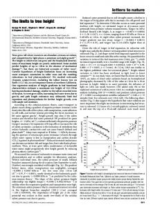
in T . Then x and y are unrelated in T i� C is a cutset in G such that x and y are in di�erent components of G ? C . Proof. Let s be the child of z such that x 2 T [s]. We know from Fact 1 that the nodes in T [s] induce a connected component G0 of G. ) 1 Since adj (G0 ) � C (Fact 2) and y 62 C it follows that y 62 adj (G0 ). We know that y 62 G0 ; adj (G0 ) must therefore be a cutset between x and y in G. ( Because G0 is connected we know that y 62 T [s]. It follows that s and y must be unrelated in T and therefore also x and y. Note the following consequence of Theorem 1: if v is an ancestor of z in T then x and y are unrelated in T i� the nodes on the path z; :::; v in T induce a cutset in the subgraph of G induced by the nodes in T [v]. Nested Dissection is a top down algorithm where one rst identi es and removes a cutset from G. The nodes in the cutset are ordered last. This process is then repeated recursively for each remaining component. This guarantees that nodes in di�erent remaining components at each stage are unrelated in T and that at least one node in each cutset has two or more children in T . Each cutset is chosen in such a way that the largest remaining component includes no more than bcnc nodes for some constant c, 0 < c < 1, where n is the number of remaining nodes. We shall call such an elimination ordering for a cn-Nested Dissection ordering. It can be shown that if G and its subgraphs have separators of size s such that no component is larger than cn where c is some constant, then we can always nd a Nested Dissection ordering that gives an elimination tree of height O(slogn) (Bodlander et. al [1]). In [7] Leiserson and Lewis give experimental results from applying a Nested Dissection algorithm to a collection of matrices from the Harwell-Boeing collection [2]. However, as we shall see no Nested Dissection ordering will give a minimum height elimination tree for every graph. Consider the graph G in Figure 1. We have shown the two elimination trees corresponding to the following two elimination orderings: � = fa; b; c; d; f; e; h; i; gg and = fa; b; h; i; c; d; g; d; f g. Tα
G c
d
e
f
a
b
g
h
i
Tβ g
a
b
f
e d
h f
i
g a
b
d h i
c
e
c
Fig. 1.
As seen from Figure 1, gives a minimum height elimination tree, while � is ordered after a Nested Dissection ordering. If we add nodes to G that are only adjacent to g we still have to eliminate e or f last in order to get a minimum height elimination tree. From this we see that for any given value of c, we can add nodes which are only adjacent to g such that the component of G ? f containing g, has more than cn nodes. Thus we see that no cn-Nested Dissection ordering will give a minimum height elimination tree for an arbitrary graph. 1
In Liu gives a proof of the ) part of Theorem 1. 3
Maximal Independent Subset is a greedy algorithm where one chooses a maximal independent set of nodes S1 (i.e. if v; w 2 S1 , (v; w) 62 E (G)) and orders rst. For each pair x; y 2 S1 the nodes in G ? S1 will be a cutset. This guarantees that exactly the nodes in S1 will be leaves in T . The process is repeated (recursively) after adding ll edges to G so that for each x 2 S1 adj (x) is a clique. Gilbert et al. [3] present an implementation of the Maximal Independent Set algorithm on the Connection Machine. As it turns out Maximal Independent Set does not in general give a minimum height elimination tree no matter how we choose Si at each stage of the algorithm. To see this look at the graph and the elimination tree in Figure 2. G
T a
b
c
b
d e g
h
i
i
j
a
k
j
e
h
f
g
d
f
c
k
Fig. 2.
The only elimination ordering that achieves minimum height 3 is given by choosing
S1 = fa; c; d; f; g; kg as leaves in T . But this is not a maximal independent set since no node adjacent to i is chosen. Thus we see that no Maximal Independent Set ordering will give a minimum height elimination tree for an arbitrary graph. Maximal Independent Set is a generalization of an algorithm for nding low elimination trees for chordal graphs by Jess and Kees [6]. At each stage in their algorithm one selects a maximal independent set of simplicial nodes and eliminate. It has been shown (Liu [8]) that for chordal graphs this algorithm give the lowest possible elimination tree over all orderings that does not increase the number of ll edges. It is however easy to see that the Jess and Kees algorithm does not produce a minimum height elimination tree for an arbitrary chordal graph if we allow ll edges. Consider a straight line of 2k ? 1 nodes. It has minimum height k ? 1, but the lowest tree one can get without increasing ll has height 2k?1 ? 1. 4. Minimal Cutset Orderings. A Minimal Cutset ordering is an elimination ordering where one removes a minimal cutset C from G and order it last (with no constraint on the size of the components of G ? C ). This is repeated (recursively) until all remaining component are cliques in G. It is easy to show that each minimal cutset C will be a non-lowest maximal chain in T and that C will induce a clique in G� . We will now show that for an arbitrary graph G with elimination tree T there exists an elimination ordering � such that the following two conditions are met: (1) � is given by a Minimal Cutset ordering. (2) h(T� ) � h(T ). We give a proof by induction on the number of nodes in G. Let G be a graph with elimination tree T . If jV (G)j � 2 the hypothesis is trivially true. Assume now that jV (G)j = n > 2 and that the induction hypothesis holds for jV (G)j < n. There are two cases to consider: 1. T is a chain. If G is a clique we are done. If G is not a clique then there must exist some minimal cutset C in G. We eliminate C last in any order. By the 4
induction hypothesis there exists an elimination order �i on each component of G ? C such that the result is true. Our elimination ordering will now be any ordering that preserves the order within each �i and with C last. 2. T is not a chain. Let K be the uppermost maximal chain in T . Note rst that reordering the nodes in K will not increase the height of the elimination tree. Since K is a cutset it must contain a minimal cutset C. Reorder K so that the nodes in C are ordered last and the nodes in K ? C second last. T .e height of the elimination tree has not increased and a minimal cutset is now eliminated last. The result now follows by the induction hypothesis. Since our claim holds true for every ordering on G we are able to state the following result: Theorem 4.1. Let G be an arbitrary graph. Then there exists a Minimal Cutset ordering on G that gives an elimination tree of minimum height. 5. The Minimal Cutset Algorithm. We will now show how the result from Theorem 2 can be utilized to design an algorithm for reducing the height of an elimination tree. We will design an algorithm that takes any elimination ordering and reorders it into a Minimal Cutset ordering giving an elimination tree of the same or lower height. To do this we rst need the following fact from Liu [9]: Fact 3. Let G be a graph with elimination tree T . A node x 2 V (G) is adjacent in G� to exactly those of its ancestors in T that the nodes in T [x] are adjacent to in G. First we look at the case when the elimination tree is not a chain. Let G be a graph with elimination tree T and let K be the set of nodes in the uppermost maximal chain in T . The new elimination ordering � is the same as the one we had originally except that we have interchanged the relative order among the nodes in K . This ensures that the height of the new elimination tree does not increase. Let x 62 K be a child of a node in K such that h(x) is maximal among all such nodes. Then we know from Fact 3 that x is adjacent in G� to all the nodes in K which the nodes in T [x] are adjacent to in G. We call this set of nodes B . It follows that B is a cutset in G. We now nd a component R of G ? B which is adjacent in G to the fewest nodes in B . The subset of B that R is adjacent to is denoted by C . Each component of G ? B which is adjacent in G to a node in B ? C is in the same component of G ? C as both x and B ? C . It follows that each component in G ? C is adjacent in G to each node in C . C must therefore be a minimal cutset in G. G B x
C
R
Fig. 3.
The nodes in K are now permuted so that we rst eliminate the nodes in K ? B followed by the nodes in B ? C and C while maintaining the relative order among the nodes in each group. This ensures that a minimal cutset is eliminated last and that 5
the height of the elimination tree does not increase. The e�ect on T is that the nodes in T [x] have now been moved jK j ? jB j places closer to the root. This process can be performed in two steps: First we eliminate the nodes in B last. This way we can identify the nodes in C by nding a node y 62 B such that p(y) 2 B and so that y is adjacent in G� to the fewest nodes in B among all such nodes. We then set C equal to the nodes in B that y is adjacent to in the current G� . Finally we rearrange the nodes in B so that the nodes in C are eliminated last. We can now remove C and all edges incident to it from G and T , and repeat the process for each remaining component. When this is done each maximal non-lowest chain v; :::; w will induce a minimal cutset in the subgraph of G induced by the nodes in T [w]. It remains to show how each maximal lowest chain in T which does not induce a clique in G, can be reordered into a Minimal Cutset-ordering such that the height of the elimination tree is not increased. Assume that G is not complete and that h(T ) = n ? 1. Then reordering the nodes cannot increase the height of T . Since G is not a clique there exists at least one node x which is not adjacent to all other nodes in G. The nodes in K = adj (x) is a cutset in G. We eliminate the nodes in K last and the nodes in V (G) ? K second last. Some node in K must now have at least two children, and we can proceed as for the maximal non-lowest chain. This method can be applied recursively to each maximal lowest chain in T until all lowest chains are cliques in G. We thus see that this algorithm which we will call the Minimal Cutset-algorithm, will nd a Minimal Cutset ordering for any graph without increasing the height of the elimination tree. Figure 4 shows an example of how the algorithm works. We start with the elimination ordering b; d; f; c; a; e. The topmost maximal chain is c; a; e and we choose x = d. This gives B = fa; cg which we order last. We then set y = e or f and get C = c which is ordered last. We now have a lowest chain b; d; a which is reordered so that b is eliminated last. G
a
b
c
d
e
f
T
e
a
a
c
c d
d f
e
b
c a
f
d
e
c f
b a
e
f
d
b
b
Fig. 4.
The height of the elimination tree is now reduced from 4 to 2. 6. Tree Rotations and Chain Reorderings. We will now study two algorithms for reducing the height of an elimination tree by respectively Liu [8] and Hafsteinsson [4] and see how they compare with the Minimal Cutset algorithm. Liu's algorithm performs local rotations in the elimination tree that do not increase the number of ll edges. The algorithm is based upon the following idea: Let x be a node such that its ancestors in T induce a clique in G� and let K be the ancestors of x which are adjacent to x in G� and B the ancestors which are not adjacent to x in G� . We now restructure the nodes in K and B so that the nodes in 6
K are ordered last and the nodes in B second last while keeping the relative order among nodes in the two groups. The rest of the ordering is kept as it is. Since K is a cutset between x and B it follows that x and B are unrelated in the new elimination tree and that T [x] has moved jB j places closer to the root of the elimination tree. The algorithm is as follows:
y = a deepest leaf in T For each x on the path root(T ); :::; y in T If x is not adjacent i G� to all of it's ancestors in T then if Restructure(x) makes T lower then Restructure(x) else Halt
Figure 5 shows an example of how the algorithm works. We set y = 1 and perform Restructure(2). This reduces the height of the elimination tree from 3 to 2. G
T
5
1 3
5
4
3
2
3 4
2
2
5
1
4
1
Fig. 5.
Hafsteinsson's algorithm reorders each maximal chain v; :::; w = K in T which is not a clique in G� . It works by selecting the topmost node x 2 K that is not adjacent in G� to all other nodes from K and by eliminating x rst while keeping the rest of the ordering as it is. Let y 2 K be the highest node not adjacent to x in G� . It follows that the ancestors of y are now a cutset between x and y in G and that x is a leaf with p(x) = p(y). This process is continued until all chains in T are cliques in G� . Figure 6 shows an example of Hafsteinsson's algorithm. We have 3 maximal chains in T but only 1,2,3 is not a clique in G� . Setting x = 2 and reordering this chain gives an elimination tree of height 2. G
T 6
6 1
2
3
6
5
4
3
5
2
4
2 1
5 3
4
1
Fig. 6.
We now show that none of the algorithms is strictly better than any of the others. Note rst that the only algorithm that has any e�ect on the original elimination tree in Figure 4 is the Minimal Cutset algorithm. Similarly the only graph that has any 7
e�ect on the graph in Figure 5 is Liu's. Finally, Liu's algorithm has no e�ect on the graph in Figure 6 and the Minimal Cutset algorithm cannot produce as low an elimination tree as Hafsteinsson's algorithm on the graph in Figure 7. In Figure 7, a shows the initial elimination tree with double lines indicating a chain of consecutive ordered nodes, b shows the elimination tree after applying Hafsteinsson's algorithm and c shows the elimination tree after applying the Minimal Cutset algorithm. T
G 5
11
8
9 10
7
1
4 6
3
2
11
8
6
4
7
5
3
1
2
6
9
5
10
3
11
4
11
2
10
3
1
2
a
b
4
9 7
c
8 1
Fig. 7.
7. A New Class. In this section we show a general result on how elimination trees can be reordered. It turns out that the three algorithms studied in the previous section are all based on special cases of this general result. Theorem 7.1. Let G be a graph with elimination ordering � and elimination tree T� . Let x; y 2 V (G) be such that y is an ancestor of x in T� and (x; y) 62 E (G�� ). Then there exists a permutation of the nodes on the path x; :::; y in T� such that exactly y is removed from the ancestors of x. Proof. Let v be the highest node on the path x; :::; y in T� such that (v; y) 62 E (G�� ). We can assume that the nodes on the path v; k1 ; k2 ; :::; kr ; y in T� are eliminated in consecutive order and that the nodes in the subtrees hanging from this path are eliminated before v. This will not a�ect the structure of T� nor the ll in G�� . We create a new elimination order by eliminating y just before v while maintaining the relative order among the rest of the nodes. Since y has no edges in G�� to nodes in T� [v] it follows that K = k1 ; k2 ; :::; kr and the ancestors of y in T� induce a cutset between y and v in G, and that v and y must be unrelated in T . The structure of T is described by the following observations: 1. Since only the order among the nodes in K [ y is altered the structure of each subtree in T� ? K ? y remains unchanged. 2. Since v; k1 ; k2 ; :::; kr?1 are eliminated in consecutive order in and each node is adjacent to the next in G� it follows that p(v) = k1 and that p(ki ) = ki+1 , 0 � i < r, in T . If p(y) 6= root(T� ) let z = p(y) in T� . Then there is some node in T� [y] that is adjacent to z in G. This node will be a descendant of kr in T . It follows that (kr ; z ) 2 E (G� ) and that p(kr ) = z in T . If y = root(T� ) then kr will be the root of T since kr is now eliminated last. 3. Let w be a node such that w 62 K and p(w) 2 K in T� . If (w; y) 2 E (G�� ) then p(w) = y in T else if (w; y) 62 E (G�� ) then p(w) remains unchanged in T . 8
4. If (k1 ; y) 62 E (G) there must be some child w of k1 in T� such that (w; y) 2 E (G�� ) and therefore also in E (G� ). In T� the node w will be a child of y. Thus (y; k1 ) 2 E (G� ) and it follows that p(y) = k1 in T . Tα
Tβ
z
z kr
y
kr
k1
k1
y
v
v
x
x
Fig. 8.
From observations 1 to 4 it follows that the path x; :::; root(T� ) remains unchanged in T except that y has now been removed. We can view the process used in the proof of Theorem 3 in the following way: After we have selected x and y we move y downwards in T until it folds out to the side. We will now show that the three algorithms from the previous section consist of repeated applications of this result. First consider the Minimal Cutset algorithm. Note that in both steps (selecting a cutset and making it minimal) of the reordering of a non-leaf chain in the Minimal Cutset algorithm we select a set of related nodes (K ? B and B ? C ) which are removed from the ancestors of some node (x and y). The reordering step can be viewed as if the nodes in each set are moved down one at a time until they fold out starting with the lowest node rst just like in the proof of Theorem 3. In Liu's algorithm the reordering step consists of selecting a set of nodes B which are not adjacent to some node x on a longest path in T . In the same way as for the Minimal Cutset algorithm these nodes are moved down starting with the lowest node rst, until they fold out. Hafsteinsson's algorithm is just an application of Theorem 3 with the restriction that the path from x to y in T must be a maximal chain. We thus see that the algorithms di�er as to the strategy by which the nodes to be folded out are selected. When applying the result from Theorem 3 it is not true that the height of the elimination tree always decreases. This is still not true even if we select x on a longest path in T and fold out an ancestor y of x which is not adjacent to x in G� . This is so because on its way down y will pull with it all subtrees that are hanging on the path x; :::; y in T that are adjacent to y in G� (observation 3 in Th. 3). These will now be further down in the elimination tree than before. If w is a node hanging from the path p(v); :::; y in T with (w; y) 2 E (G� ) and if h(w) � h(v) then the height of the elimination tree does not decrease. We can, however, continue recursively to reorder T [y] in the new elimination tree and try to make it lower. None of the algorithms uses the result of Theorem 3 to its full extent for reducing height. In order to see this look at the graph in Figure 9. None of the three algorithms gives a lower elimination tree. Node 9 is not adjacent to node 2 in G� . We can therefore move node 9 down until it folds out and in doing so produce a lower elimination tree. 9
G 1
T 3
6
5
9
8
8
6
4
8 2
6
7
3
5
7 9
3
5
2
9
2
4
1
7
4
1
Fig. 9.
Di�erent ways of selecting the nodes to be folded out can lead to other algorithms. Let x be a node on a longest path in T . Other choices might be: 1. Fold out the lowest/highest eligible node. 2. Fold out the node that has to be moved the shortest distance. 3. Fold out the node that is closest to the root after having been folded out. 8. Conclusion. We have shown that Nested Dissection and Maximal Independent Subset give potentially low elimination trees but not necessarily of minimum height. We have also introduced a more general class of elimination orderings called Minimal Cutset orderings and shown the existence of a Minimal Cutset ordering that gives a minimum height elimination tree for an arbitrary graph. This result is useful since it tells us that it is only necessary to remove minimal cutsets when doing Nested Dissection on a graph in order to get a low elimination tree. It can also be helpful when designing algorithms for nding minimum height elimination trees for special classes of graphs. One such an algorithm for trees is shown by the author in [11]. We then compared the algorithms proposed by Liu and Hafsteinsson with the Minimal Cutset algorithm and showed that none of these is strictly better than any of the others. Finally, we showed that these three algorithms are members of a class of algorithms that depend on a general result on how elimination trees can be reordered. Bodlander et al. [1] has shown that an approximation algorithm for nding cutsets can be used to nd an elimination tree which is at most of height log2n times the minimum. It would be interesting if one could nd orderings which at the same time keep the amount of ll low and also gives a low elimination tree. If one is to achieve a low elimination tree there cannot be too much ll in G� since it would increase the dependencies among the nodes and prevent branching. Heggernes [5] has shown that given a partition of a graph into minimal cutsets nding the minimum ll ordering reduces to a local problem for each, but unfortunately these problems still remain NP-hard. 9. Acknowledgments. The author thanks Professor Bengt Aspvall for encouragement and guidance during the work with [10] where most of the results of this paper were rst presented.
10
REFERENCES [1] H. L. Bodlander, J. R. Gilbert, H. Hafsteinsson, and T. Kloks, Approximating treewidth, pathwidth and minimum elimination tree height, Tech. Report CSL-90-10, Xerox Palo Alto Research Center, 1991. [2] I. Duff, R. Grimes, and J. Lewis, Sparse matrix test problems, ACM Transactions on Mathematical Software, 15 (1989), pp. 1{14. [3] J. R. Gilbert and R. Schreiber, Highly parallel matrix reordering and symbolic factorization. In preparation, 1991. [4] H. Hafsteinsson, Parallel Sparse Cholesky Factorization, PhD thesis, Cornell University, 1988. [5] P. Heggernes, Reducing the ll-in size for an elimination tree. University of Bergen, Norway, In preparation, 1991. [6] J. A. G. Jess and H. G. M. Kees, A data structure for parallel LU decomposition, IEEE Transactions on Computers, C-31 (1982), pp. 231{239. [7] C. E. Leiserson and J. G. Lewis, Orderings for parallel sparse symmetric factorization. Unpublished manuscript, 1988. [8] J. W. H. Liu, Reordering sparse matrices for parallel elimination, Parallel Computing, 11 (1989), pp. 73{91. [9] , The role of elimination trees in sparse factorization, SIAM Journal of Matrix Analysis and Applications, 11 (1990), pp. 134{172. [10] F. Manne, Minimum height elimination trees for parallel Cholesky factorization, master's thesis, University of Bergen, Norway, 1989. (In Norwegian). , An algorithm for computing a minimum height elimination tree for a tree, Tech. Report [11] CS-91-59, University of Bergen, Norway, 1992. [12] A. Pothen, The complexity of optimal elimination trees, Tech. Report CS-88-13, Pennsylvania State University, 1988. [13] M. Yannakakis, Computing the minimum ll-in is NP-complete, SIAM Journal of Algorithms and Discrete Methods, 2 (1981), pp. 77{79.
11