Reducing the number of points on the convex hull ... - MeshFree

Reducing the number of points on the convex hull calculation using the polar space subdivision in 𝐸 2 Vaclav Skala, Michal Smolik, Zuzana Majdisova Department of Computer Science and Engineering, Faculty of Applied Sciences University of West Bohemia Plzen, Czech Republic Email: {skala, smolik, majdisz}@kiv.zcu.cz Abstract—A convex hull of points in 𝑬𝟐 is used in many applications. In spite of low computational complexity 𝑶(𝒉 𝐥𝐨𝐠 𝒏) it takes considerable time if large data processing is needed. We present a new algorithm to speed-up any planar convex hull calculation. It is based on a polar space subdivision and speed-up known convex hull algorithms of 𝟑, 𝟕 times and more. The algorithm estimates the central point using 𝟏𝟎% of the data; this point is taken as the origin for the polar subdivision. The space subdivision enables a fast and very efficient reduction of the given points, which cannot contribute to the final convex hull. The proposed algorithm iteratively approximates the convex hull, leaving only a small number of points for the final processing, which is performed using a “standard” algorithm. Noneliminated points are then processed by a selected standard convex hull algorithm. The algorithm is simple and easy to implement. Experiments proved numerical robustness as well. Keywords—Convex hull; iterative approximation; space subdivision; reduction of points;

𝑂(𝑛 log 𝑛) lower bound, every convex hull algorithm must require 𝑂(𝑛 log 𝑛) time for some inputs. Despite these matching upper and lower bounds, and probably due to the many applications of convex hulls, a number of other planar convex hull algorithms have been published since Graham’s algorithm. Moreover, the Marriage before Conquest algorithm (Kirkpatrick and Seidel, 1986) computes the convex hull in 𝑂(𝑛 log ℎ) time, where ℎ is the number of vertices of the final convex hull. The same authors showed that, on algebraic decision trees of any fixed order, 𝑂(𝑛 log ℎ) is a lower bound for computing convex hulls of a set of 𝑛 points, having a convex hull with ℎ vertices. Table 1. Comparison of 2D convex hull algorithms and their time complexity. The number of input points is 𝑛 and ℎ is the number of vertices of the final convex hull. Note that ℎ < 𝑛, so 𝑛ℎ < 𝑛2 .

I. INTRODUCTION

Algorithm

A convex hull was one of the first sophisticated geometry algorithms to be computed and there are many variations of it. The most common form of this algorithm involves the determination of the smallest convex set, called the "convex hull", containing a discrete set of points. There are numerous applications for convex hulls: collision avoidance, maximum distance using convex hull diameter for large data sets (Skala, 2013), (Skala and Majdisova, 2015), hidden object determination, and shape analysis, point inside polygon (Skala and Smolik, 2015), to name a few.

Gift Wrapping Graham Scan Jarvis March QuickHull Divide & Conquer Monotone Chain Incremental Marriage before Conquest Chan's algorithm Ordered hull

Expected time complexity 𝑂(𝑛ℎ) 𝑂(𝑛 log 𝑛) 𝑂(𝑛ℎ) 𝑂(𝑛ℎ) 𝑂(𝑛 log 𝑛) 𝑂(𝑛 log 𝑛) 𝑂(𝑛 log 𝑛)

(Chand and Kapur, 1970) (Graham, 1972) (Jarvis, 1973) (Eddy, 1977), (Bykat, 1978) (Preparata and Hong, 1977) (Andrew, 1979) (Kallay, 1984)

𝑂(𝑛 log ℎ)

(Kirkpatrick and Seidel, 1986)

𝑂(𝑛 log ℎ) 𝑂(𝑛 log ℎ)

(Chan, 1996) (Liu and Chen, 2007)

Reference

II. PROPOSED ALGORITHM

A subset 𝑆 ⊆ ℝ2 is convex if and only if for any two points 𝒑, 𝒒 ∈ 𝑆 the line segment with endpoints 𝒑 and 𝒒 is completely contained in 𝑆. The convex hull 𝒞ℋ(𝑆) of a set 𝑆 is the smallest convex set that contains 𝑆. To be more precise, it is the intersection of all convex sets that contain S. The convex hull of a set of points 𝑃 is a convex polygon with vertices in 𝑃.

In the following section, we will introduce a new approach to speeding any convex hull computation in 𝐸 2 . The main idea of this algorithm is to discard as many points as possible before the actual convex hull calculation takes place. The technique used in this algorithm is based on division of space into several polar sectors.

A. Time Complexity The search for the fastest algorithm is a pursuit which has been preoccupying many authors for many years now. Many have found excellent algorithms. Lately performance reached 𝑂(𝑛 log ℎ) complexity where ℎ is the number of points forming the convex hull and 𝑛 is the number of input points.

In section 2.A, we will show the first step of the algorithm proposed which is the location of points inside the created initial polygon. In section 2.B, we will show how to divide points into polar shaped sectors. In section 2.C, we will show how to reduce the suspicious points. And finally, in section 2.D, we will show a algorithm for calculation of the convex hull from the selected divided points.

There are many well-known algorithms used for the calculation of convex hull in 2𝐷. A comparison of the time complexity for some of them can be seen in Table 1. (Graham, 1972) gave a complex hull algorithm with 𝑂(𝑛 log 𝑛), the worst-case running time. Later it was shown that, in any model of computation where sorting has an

A. Location of Points inside Polygon An important property of input points is that the most extreme point on any axis is part of a convex hull. This fact is apparent if we consider an example in which an extreme point is not in the convex hull. This would mean the perimeter of

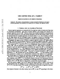
the convex hull passes through a point less extreme than that point. However, it is then obvious that the extreme point would not be included in the enclosed set, thus breaking a fundamental characteristic of convex hulls. This property is used in our algorithm for speeding-up the creation of the convex hull. The first step is finding the axis aligned bounding box (AABB) of the input points, which is of 𝑂(𝑛) time complexity. For the future described polar space subdivision we do not need the exact extremal point, close enough extremal points are sufficient for our purpose. Therefore we do not have to search for them through all the input points, i.e. we can search only approximately 10% of all points. This simplification can save us some time and will not cause any disadvantage in future calculations. So we get four distinct points or, in some cases, only three or even just two. Using these points we can create a convex polygon, see Fig. 1. One important property of this polygon is that any of the points lying inside cannot be the points of the final convex hull. Keeping this in mind, we can create the initial test for determining whether the point is inside/outside the polygon and dismiss a lot of points by using this easy initial test.

One way to divide the space is to use a uniform division of an angle from 0 to 2𝜋. Using this, we have to calculate the exact angle between the vector 𝒙′ = [0, 1]𝑇 and the vector 𝒗 = 𝒙 − 𝑪, and such a calculation uses the following formula: (2)

𝜑 = arctg2(𝒗𝑥 , 𝒗𝑦 ) .

Calculation of the function arctg2(𝒗𝑥 , 𝒗𝑦 ) takes a lot of time and we therefore use a simplified calculation of the approximated angle. The simplified angle is not uniformly distributed on a circle, but it is uniformly distributed on the border of a square 〈−1, −1〉 × 〈1,1〉 . When calculating the angle, we have to locate the exact half of quadrant, i.e. octant, where the point is located, and then calculate the intersection with the given side. The intersection with a side is simple, as all sides of the box’s axis are aligned and intersect with the main axes at 𝑦 or 𝑥 = 1 or − 1. The distribution of a simplified angle can be seen on Fig. 2.

Fig. 2. Uniform distribution of a simplified angle on a unit square. Angle 𝜑 ∈ 〈0,8〉 instead of 〈0,2𝜋〉. a)

b)

c) 4

Fig. 1. Location of initial inner testing polygon inside the convex hull for 10 points (10% of points used for finding AABB box): a) uniform points in circle, b) uniform points in square, c) Gauss points.

Calculation of a simplified angle is faster than the formula (2) and gives almost the same results, as can be seen in Fig. 3.

The location test of a point inside a polygon can be determined using the following steps. Each side of the polygon is an oriented line and thus we can calculate 𝐹𝑖 (𝒙), where 𝒙 is the point and 𝐹𝑖 (𝒙) = 0 is the implicit formula for a side with index 𝑖: a)

𝐹𝑖 (𝒙) = 𝑎𝑖 𝑥 + 𝑏𝑖 𝑦 + 𝑐𝑖 = 0 .

b)

c)

(1)

If 𝐹𝑖 (𝒙) < 0 for at least one 𝑖 ∈ {1, … ,4} then the point 𝒙 lies outside of the polygon and has to be used for further processing. Thus if for all 𝑖 ∈ {1, … ,4} is 𝐹𝑖 (𝒙) ≥ 0 then the point 𝒙 lies inside of the polygon and can be discarded. B. Division of Points into Sectors Some points were discarded because of their location inside the inner polygon. Other points have to be further processed. The 2𝐷 space can be divided into several non-overlapping polar shaped sectors. This division uses a center point and angular division. Center point 𝑪 is calculated as the average of all corners of the inner initial polygon.

Fig. 3. Division of space into 32 (a), 64 (b) and 128 (c) non-overlapping sectors using uniform distribution of a simplified angle.

Now we have a simple calculation of the simplified angle and therefore we are able to determine the index of the sector to which the point belongs. Each sector with the index 𝑖 contains one maximum point 𝑹𝑚𝑎𝑥 . This point has the maximum (from all points in a 𝑖 sector) distance from the center point 𝑪. The initial points 𝑹𝑚𝑎𝑥 lies on the sides of the initial polygon, (see Fig. 4). We 𝑖 can calculate 𝑹𝑚𝑎𝑥 as an intersection point of the middle axis 𝑖 of a sector and the polygon side.

All maximum points 𝑹𝑚𝑎𝑥 form a polygon with vertices 𝑖 …, 𝑹𝑚𝑎𝑥 , where 𝐾 is count of all sectors (i.e. space 𝐾 division count). 𝑹1𝑚𝑎𝑥 ,

For each new point we have to check whether the distance from the center 𝑪 is greater than the distance for 𝑹𝑚𝑎𝑥 from 𝑖 the center 𝑪. If it is true, then we have to replace the maximum point 𝑹𝑚𝑎𝑥 with the actual point, recalculate lines 𝑖 𝑙 + and 𝑙 − , (see Fig. 5) and add this point into the sector with index 𝑖. Otherwise, we have to continue with the next step.

Fig. 4. Visualization of initial 𝑅𝑖𝑚𝑎𝑥 points (red dots on the sides of the initial polygon).

The next step is to check whether the point lies over or under line segments 𝑙 + and 𝑙 − , (see Fig. 5). We can compare the angle of the point with the angle of 𝑹𝑚𝑎𝑥 . If the angle is 𝑖 greater, then we have to use the line 𝑙 + , otherwise we have to use the line 𝑙 − . If the point is under the line 𝑙 + , or 𝑙 − , we can discarded it, because such a point cannot be part of the convex hull. Otherwise we have to add that point into the list of points associated with the segment with index 𝑖.

Fig. 5. Visualization of lines 𝑙− and 𝑙+ .

computation is therefore not significant compared to the time required for the reduction of all the original input points. We can therefore use any algorithm for convex hull creation and not necessarily the fastest one. We chose to use the Graham Scan algorithm. The input set of points for convex hull computation is subdivided into sectors. We can utilize the partial ordering of points in order to speed-up the convex hull algorithm. The first step of the Graham Scan is to sort all points in increasing order of the angle between vector 𝒙′ = [0, 1]𝑇 and the vector 𝒗 = 𝒙 − 𝑪, where the point 𝑪 is the center point of the initial polygon and 𝒙 is the point. All of these angles have already been precomputed from the point division phase and we do not have to compute them once more. The sorting process is done for each sector separately and then only the sorted groups of points are joined into one sorted array. The Graham Scan needs one initial point which will be on the convex hull. We have to find the point with the highest 𝑥 coordinate. This step takes 𝑂(𝑀), where 𝑀 is the number of the suspicious points (the input points for this part of convex hull creation). The algorithm proceeds by considering each of the points in the sorted array in sequence. For each point, it is determined whether moving from the two previously considered points to this point is a “left turn” or a “right turn”: ≥0 [(𝑩 − 𝑨) × (𝑪 − 𝑨)]𝑧 {