Reexamining Adaptation and the Set Point Model of ... - CiteSeerX

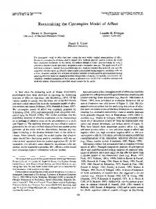
Journal of Personality and Social Psychology 2003, Vol. 84, No. 3, 527–539

Copyright 2003 by the American Psychological Association, Inc. 0022-3514/03/$12.00 DOI: 10.1037/0022-3514.84.3.527

Reexamining Adaptation and the Set Point Model of Happiness: Reactions to Changes in Marital Status Richard E. Lucas

Andrew E. Clark

Michigan State University

De´partement et Laboratoire d’Economie The´orique et Applique´e

Yannis Georgellis

Ed Diener

Brunel University

University of Illinois at Urbana–Champaign

According to adaptation theory, individuals react to events but quickly adapt back to baseline levels of subjective well-being. To test this idea, the authors used data from a 15-year longitudinal study of over 24,000 individuals to examine the effects of marital transitions on life satisfaction. On average, individuals reacted to events and then adapted back toward baseline levels. However, there were substantial individual differences in this tendency. Individuals who initially reacted strongly were still far from baseline years later, and many people exhibited trajectories that were in the opposite direction to that predicted by adaptation theory. Thus, marital transitions can be associated with long-lasting changes in satisfaction, but these changes can be overlooked when only average trends are examined.

& Tellegen, 1996). According to this idea, people have happiness set points to which they inevitably return following disruptive life events (Headey & Wearing, 1989; Larsen, 2000; Williams & Thompson, 1993). Some researchers have gone so far as to argue that adaptation processes are so strong that trying to change one’s happiness is futile because an individual inevitably returns to a genetically predetermined state (Lykken & Tellegen, 1996). Yet questions about adaptation remain. Although a number of studies have shown evidence for the adaptation phenomenon, most existing studies have limitations that prevent researchers from drawing strong conclusions about the extent to which people adapt. In the current study, we use data from a large-scale, longitudinal study to test whether people adapt to changes in marital status. Specifically, we examine whether levels of life satisfaction (one of the major components of SWB) return to baseline levels following marital events. The goal of this study is to test whether adaptation does or does not occur. We wish to establish whether the pattern exists, and, at this point, we make no claims about the processes that may underlie these effects.

In their classic article on adaptation, Brickman and Campbell (1971) argued that people are confined to a hedonic treadmill— they are doomed to experience stable levels of well-being because, over time, they adapt to even the most extreme positive and negative life circumstances. This idea has received considerable empirical support. Most cross-sectional studies of life satisfaction and long-term emotional levels find that objective circumstances account for surprisingly little variance in reports of subjective well-being (SWB). Even people who have won large sums of money in lotteries and people who have experienced debilitating injuries appear not to differ strongly from the average person (Brickman, Coates, & Janoff-Bulman, 1978). Thus, although people may react strongly to life events, the evidence suggests that they eventually return to their initial levels of happiness. The hedonic treadmill theory has had a profound effect on SWB research (for general reviews of the area, see Argyle, 1987; Diener, Suh, Lucas, & Smith, 1999; Kahneman, Diener, & Schwarz, 1999; Lyubomirsky, 2001; Myers, 1993). The theory’s supporting evidence has led some researchers to conclude that adaptation is quick, complete, and inevitable and that most of the long-term stable variance in SWB can be accounted for by personality and genetic predispositions rather than by life circumstances (Lykken

Previous Research on Adaptation Although adaptation is a dynamic process, few studies have examined the dynamic nature of the phenomenon. Instead, most evidence for adaptation comes from single-occasion crosssectional studies (see Frederick & Loewenstein, 1999, for a review). For example, in one of the most famous adaptation studies, Brickman et al. (1978) examined the SWB of lottery winners and persons with spinal-cord injuries. They found that lottery winners were less happy than would be expected (and nonsignificantly happier than a control group) and that individuals with spinal-cord injuries were happier than might be expected. A number of limitations, however, prevented the authors’ data from offering strong support for adaptation. First, although the small sample of lottery winners was not significantly happier than a control group, these individuals were slightly happier. Second, contrary to adaptation-

Richard E. Lucas, Department of Psychology, Michigan State University; Andrew E. Clark, De´partement et Laboratoire d’Economie The´orique et Applique´e, Paris, France; Yannis Georgellis, Department of Psychology, Brunel University, Uxbridge, Middlesex, England; Ed Diener, Department of Psychology, University of Illinois at Urbana–Champaign. The data used in this article were made available to us by the German Socio-Economic Panel Study at the German Institute for Economic Research, Berlin, Germany. Correspondence concerning this article should be addressed to Richard E. Lucas, Department of Psychology, Michigan State University, East Lansing, Michigan 48824, or to Ed Diener, Department of Psychology, University of Illinois, 603 East Daniel Street, Champaign, Illinois 61820. E-mail: [email protected] or [email protected] 527

528

LUCAS, CLARK, GEORGELLIS, AND DIENER

theory expectations, individuals with spinal-cord injuries were significantly and substantially less happy than the comparison group, even if they were not quite as unhappy as one might expect. Third and perhaps most important, the data were not longitudinal, which prevented Brickman et al. from comparing respondents’ postevent levels of well-being with their preevent levels. Without this information, it is difficult to interpret their results. Individuals with spinal-cord injuries might have been young, active athletes before their injury, and, thus, they might have had higher than average well-being. If so, their lower than average life satisfaction may reflect a very large drop from preinjury levels. Thus, Brickman et al.’s elegant study is intriguing, but it does not offer definitive support for the idea of adaptation. Subsequent studies have improved on Brickman et al.’s (1978) research design, and these studies provide stronger evidence that some form of hedonic adaptation does occur. Silver (1982), for example, followed individuals with spinal-cord injuries from 1 to 8 weeks after the accident that produced their disability. One week after the misfortune, negative emotions were stronger than positive emotions. Over the next 7 weeks, negative emotions decreased, and happiness increased. By the 8th week, positive emotions were stronger than negative emotions. These longitudinal data offer support for some degree of adaptation, though it is unclear whether respondents ever returned to their preaccident baseline levels of SWB. To capture the complete process of reaction and adaptation to events, it is desirable to study large groups of individuals for long periods of time. Inevitably, some of the individuals being studied will experience major life events, and then researchers can determine whether adaptation occurs. One study that used this design is Headey and Wearing’s (1989) Australian Panel Study. These authors followed a group of respondents for a period of 8 years. They found that people initially reacted strongly to bad and good events but then returned toward their original baseline levels of SWB. On the basis of their data, Headey and Wearing (1989) made several modifications to the original hedonic treadmill hypothesis. In their dynamic equilibrium model, Headey and Wearing proposed that people appear to have baseline moods in the positive range and that individuals return to differing baselines, depending on their personalities. Furthermore, Headey and Wearing showed that happy people were more likely than unhappy people to experience good events and that unhappy people were more likely than happy people to experience bad events. Thus, they argued, one’s baseline is due, in part, to the fact that certain individuals are more or less likely to experience certain affect-inducing events. Although Headey and Wearing (1989) provided strong evidence that adaptation does occur, their study could not resolve a number of important questions about the process. First, it is still unclear whether adaptation to events is complete. Do people always return to the same baseline, or are new baselines created following major life events? Second, although Headey and Wearing showed that there are individual differences in baseline levels of mood and individual differences in the tendency to experience events, they did not examine whether there are individual differences in the extent to which people adapt. Are there certain individuals who show no adaptation? And, finally, if individual differences in adaptation do exist, we can ask whether there are any factors that predispose people to more or less complete adaptation. Specifically, a number of researchers have suggested that happy individuals react more strongly to pleasant stimuli and that unhappy

individuals react more strongly to unpleasant stimuli (e.g., Gable, Reis, & Elliot, 2000; Larsen & Ketelaar, 1991). If this reactivity hypothesis is true, individuals who have high baseline levels of SWB should react more positively to positive marital transitions (e.g., getting married), whereas individuals who have low baseline levels of SWB should react more negatively to negative marital transitions (e.g., becoming widowed). In addition, we can determine whether other individual-level factors (e.g., age and sex) moderate reaction and adaptation to marital transitions. In the present study, we attempt to answer these questions by examining adaptation to changes in marital status.

The Importance of Marital Transitions Changes in marital status are among the most important transitions in the social life of adults. Indeed, in their classic article on life events, Holmes and Rahe (1967) listed widowhood and divorce as the two most stressful events in adulthood, and both events were rated as being more stressful than going to jail. It is interesting that although people tend to think of marriage as a positive event, it ranked 7th place among the 50 stressful events Holmes and Rahe listed. It is clear, however, that marriage can also be extremely rewarding and can have positive effects on SWB. In large, representative samples, married respondents reliably report higher SWB than do unmarried respondents (e.g., Glenn, 1975; Lee, Seccombe, & Shehan, 1991; see Waite, 1995, for a general discussion of the benefits of marriage). Furthermore, the relation between marital status and SWB is robust. It is not limited to certain populations, and it does not disappear when a variety of other demographic characteristics are controlled. For example, Diener, Gohm, Suh, and Oishi (2000) found evidence for the robustness of this relation in probability samples from 42 diverse nations around the globe (also see Stack & Eshleman, 1998), and Mastekaasa (1993) showed that this relation does not seem to be weakening over time. Haring-Hidore, Stock, Okun, and Witter (1985) conducted a metaanalysis of the literature and demonstrated that, on average, there is a positive association between marriage and SWB (though marital status only accounted for about 2% of the variance in well-being reports in their meta-analysis). Other researchers have shown that the association between marriage and SWB persists even when variables such as income and age are controlled (e.g., Clark & Oswald, 1994; Glenn & Weaver, 1979; Gove, Hughes, & Style, 1983). Researchers have noted that there are at least three possible explanations for the association between marital status and SWB, each of which has distinct implications for theories of adaptation (for a review, see Johnson & Wu, 2002). According to the selection hypothesis, psychological characteristics predispose certain people to experience marital events (Mastekaasa, 1992). Happy people may be more pleasant and outgoing, and these people may be more successful in finding and attracting a mate. Unhappy individuals, on the other hand, may be more likely to suffer from psychological problems that prevent them from getting married or that lead to separation and divorce. If selection effects can account for the association, then we should not expect to find adaptation effects following marital transitions. Instead, differences in wellbeing should be apparent long before the person experiences the event, and they should be stable after the event has occurred. There appears to be mixed support for the selection hypothesis. Maste-

ADAPTATION

kaasa (1992), for example, found evidence of selection effects in a cross-sectional study of 9,000 individuals in Norway (also see Mastekaasa, 1994a), but Johnson and Wu (2002) found that selection effects could not account for much of the association between marital status and SWB in a panel study spanning 12 years. A number of other studies that examine the selection hypothesis are limited by small sample sizes and short measurement periods (e.g., Menaghan, 1985; Menaghan & Lieberman, 1986). In contrast to the selection explanation, social role explanations posit that marriage, divorce, and widowhood are differentially associated with specific types of hardships (Mastekaasa, 1994b). Divorced individuals, for example, may be less likely than married individuals to have strong networks of social support, and they may be more likely to have greater financial difficulties. According to the social role explanation, these additional hardships can account for differences in SWB. Johnson and Wu (2002) argued that if social roles could account for the relation, then there should be little evidence for adaptation. If the features of the role are constant and these features have a constant effect on SWB, then SWB should not change over time. In support of the social role theory, Johnson and Wu found evidence for lasting effects of divorce on psychological distress. However, it is unclear whether people should also exhibit adaptation to these stable features of the role. Existing literature on adaptation suggests that people can adapt to a wide variety of conditions (Frederick & Loewenstein, 1999), even those that cause long-lasting changes to the day-to-day activities of one’s life (e.g., becoming a quadriplegic). Thus, we disagree that adaptation effects are incompatible with the role theory, though we agree with Johnson and Wu that evidence for long-lasting changes following marital events would lend support to the theory’s basic premise. The final explanation for the association between marital status and SWB, the crisis or event explanation, is most relevant to discussions of adaptation. According to this theory, marital transitions are disruptive and cause short-term changes in SWB. As people adapt to the transition, however, SWB levels should return to previous levels. This model explicitly predicts that adaptation should occur and that differences in well-being among people from different marital groups should disappear when time since the event is controlled. However, support for this model has also been mixed. In a study of reaction to divorce, for example, Booth and Amato (1991) found that distress increased as one approached the time of divorce and then rebounded back toward initial levels following the divorce, but Johnson and Wu (2002) used the same data set (with an additional wave and a different statistical model) and found that there were no significant effects of time since divorce. Most studies of bereavement processes work from the crisis model (e.g., McCrae & Costa, 1993; Stroebe & Stroebe, 1987), and these studies generally find evidence of adaptation over time (see Bonanno & Kaltman, 1999; Jacobs, 1993, for reviews). Similarly, long-term studies of marital satisfaction often find decreasing levels during the initial years of marriage (though these satisfaction levels usually rebound in later stages of the marriage; for a review, see Argyle, 1999). Although some longitudinal marriage studies exist, these studies generally focus on the predictors of divorce, remarriage, quality of marriage, and marital satisfaction (e.g., Bradbury, Cohan, & Karney, 1998; Bulcroft, Bulcroft, Hatch, & Borgatta, 1989; Lindahl, Clements, & Markman, 1998; Mastekaasa, 1994a). In addition, many of these studies suffer from limitations that make the study

529

of adaptation impossible. Many studies recruit dating, engaged, or recently married couples, and therefore they cannot isolate preexisting baseline levels of satisfaction (Burgess & Wallin, 1953; Hill & Peplau, 1998; Kelly & Conley, 1987; Kurdek, 1998; Lindahl et al., 1998). Longitudinal studies that do not specifically select for marriage or widowhood often have small numbers of measurement occasions (e.g., Johnson & Wu, 2002, assessed individuals only four times over the course of 12 years). Furthermore, existing longitudinal studies generally do not examine the extent to which adaptation is complete (an important goal of the current study), and very few, if any, examine individual differences in these patterns. In their review of the literature on marital dysfunction, Bradbury et al. (1998) argued that researchers should not work from the assumption that “all spouses are created equal” (p. 283). Instead, they suggested, researchers should acknowledge the importance of individual differences in the course of reaction and adaptation to marital events. In the current study, we follow this advice and examine both average trends and individual differences in life satisfaction following marital events.

Overview of Major Purposes The current study allows us to address two sets of questions about reaction and adaptation to changes in marital status. First, it allows us to better understand the association between marital status and life satisfaction. By following individuals over time, we can determine the extent to which selection effects, social roles, or crisis explanations can account for the association. Second, the current study allows us to address a series of related questions about the adaptation process more generally. By examining whether these important life events have long-lasting effects on satisfaction, we can determine whether adaptation does, indeed, occur. In addition, we go beyond previous studies by examining whether adaptation toward initial baseline levels is partial or complete. Then we can determine whether there are individual differences in the tendency to adapt. Finally, we can test whether individual differences in reaction and adaptation can be predicted from individual-level variables (including sex, age, and initial levels of satisfaction).

Method Sample The data in this study come from Waves 1–15 of the German SocioEconomic Panel Study (GSOEP), a longitudinal survey of private households and individuals living in Germany (see Haisken-De New & Frick, 1998, for a detailed description of the study and its sample). The sample consists of four separate subsamples: (a) 11,791 residents of West Germany, (b) 4,631 foreigners living in West Germany, (c) 5,329 residents of East Germany, and (d) 3,012 immigrants to West Germany. Subsamples a and b entered the study in 1984, Subsample c entered the study in 1990 (after the fall of the Berlin Wall in 1989), and two separate groups of Subsample D entered the study in 1994 and 1995. Households were contacted through a multistage random sampling technique. Various locations within Germany were randomly selected, and then households within each area were randomly contacted by an interviewer (this sampling strategy varied somewhat for the various subsamples; see Haisken-De New & Frick, 1998, for more details). Response rates varied from 60% to 70% across subsamples, a rate that is very high for this type of survey. Haisken-De New and Frick reported that the demographic characteristics of the samples are similar to the characteristics of the

530

LUCAS, CLARK, GEORGELLIS, AND DIENER

general populations from which they were drawn, which illustrates that the sampling technique was successful in drawing a representative sample. All individuals within a household who were at least 16 years old were asked to participate. Surveys were conducted in face-to-face interviews when possible, and participants were contacted yearly. A variety of strategies were used to encourage continued participation over the years. Participants were given gifts, entered into lotteries, and given information about results. In addition, when possible, the same interviewer contacted households each year, a feature that was meant to increase participants’ commitment to the study. Participants who were unavailable during one wave were contacted in subsequent years when possible, and various efforts were made to locate participants who had moved. Attrition was very low from year to year: Among the participants who began the survey in 1984, yearly attrition ranged from a high of 13.9% (from the 1st to the 2nd year) to a low of 4.3%. Average yearly attrition for this group was 6.2% per year. Yearly attrition rates among groups that started the survey in later years were similar to the group that started in 1984, ranging from 3.6% to 11.8% per year.

Measures In addition to answering a variety of demographic questions (including marital status, the primary independent variable of interest in the current study) and questions about employment and income (the GSOEP is primarily a study of economic conditions), participants indicated how satisfied they were with their life in general, using a scale that ranged from 0 (totally unhappy) to 10 (totally happy). Preliminary analyses of the life satisfaction variable indicated that average satisfaction varied significantly across years and across samples. Specifically, among West Germans and foreigners living in West Germany, life satisfaction decreased in the years preceding the fall of the Berlin Wall, rebounded in the years immediately following the fall, and then gradually decreased again after 1993. Among East Germans, life satisfaction was highest in 1990 and lowest in 1991 but increased slightly from 1992 until 1998. In addition, the East German subsample reported lower average life satisfaction than did the other three samples. To control for these differences, all life satisfaction scores were centered around the mean life satisfaction score for each group within each year.

Analytic Technique The goal of this article is to examine within-subject trends in life satisfaction following major social life events. To accomplish this goal, we used a multilevel modeling approach (using hierarchical linear modeling [HLM] software; Raudenbush, Bryk, & Congdon, 2000), with separate within-subject and between-subjects levels (for an introduction to multilevel modeling, see Bryk & Raudenbush, 1992; Kreft & De Leeuw, 1998). This flexible multilevel modeling approach has a number of advantages. First, it is appropriate for the nested nature of our data: Individual observations over time are nested within persons. Second, it does not require that all individuals be measured at all occasions. We can use the data from participants who entered the study after it began (e.g., East German and immigrant samples) and from participants who have missing data for some waves of the study. Third, it allows us to estimate within-subject and between-subjects effects simultaneously. For example, we can examine the within-subject effects of getting married and adapting to marriage, and we can then test whether subject-level variables such as age, sex, and initial level of satisfaction moderate these effects. Finally, a multilevel modeling approach allows us to specifically test the difference in fit of competing models. This enables us to test whether certain within-subject parameters, such as a separate adaptation parameter following years of marriage, can be removed from our models. For each event (marriage and widowhood), analyses proceed in the following manner. First, we identify participants who experienced the event at some point during the 15 waves of the study. Next, we restrict this

sample to those participants who did not experience a subsequent change in marital status. For example, when examining the effects of marriage, we restrict our analyses to those individuals who started the study unmarried, got married at some point during the study, and then stayed married for the duration of the study. Because we wish to examine the effects of adaptation to a specific event, we must eliminate from our analyses those participants who experienced subsequent events that nullify the initial event itself. Participants cannot continue to adapt to the event of marriage if the marriage is no longer intact.1 Of course, this means that our estimates of the changes in life satisfaction that occur only generalize to other similar groups. So, for example, the within-subject effect of marriage that we estimate must be interpreted as the within-subject effect of marriage among married couples who stay together. We note, however, that the vast majority of people who got married or became widowed met our selection criteria, and when we included all participants who experienced an event in our analyses, the results were similar and our conclusions did not change (we discuss these points in more detail when interpreting the results). Once our sample is defined, we test a simple null model. At the within-subject level, this model consists of a person’s average life satisfaction (␤0) plus random variability around this average (representing within-subject variability), and at the between-subjects level, the model consists of an overall average (␥00) plus random variability around this average (representing the between-subjects variability in average levels of life satisfaction). Then we can test how much variance is explained when various within- and between-subjects variables are added to the model. To do this, we add a dummy-coded variable to the model at the within-subject level. For participants who get married during the study, this variable represents whether they were unmarried (0) or married (1), and for participants who became widowed, this variable represents whether they were married (0) or widowed (1). In addition, because our initial exploratory analyses showed that people report anticipatory changes in life satisfaction in the year before an event occurs, we also add a within-subject dummycoded variable reflecting whether the current wave is the year preceding the marital event. By constructing the model in this way, we can interpret the parameters as follows: The intercept is a person’s average level of life satisfaction across all years that are at least 2 years before the marital event. This intercept reflects a person’s baseline level of satisfaction. The parameter for the previous year variable reflects the change in life satisfaction that occurs during the year before the marital event. Finally, the parameters for the married/not married and married/widowed variables reflect the change in life satisfaction that occurs when a person experiences the event. Specifically, these parameters can be interpreted as the difference between the average satisfaction in all years after the event and the average satisfaction in all years that are at least 2 years before the event. Although the above model tells us something about the within-subject associations between satisfaction and marital events, it cannot capture the changes that occur as people adapt. To examine adaptation, we must test more complicated models. We do this using three separate adaptation models, each with distinct advantages. In the first model, we allow for a short period of reactivity to the event and then assess whether a person’s long-term average level of satisfaction after an event is different from his or her average before the event. If adaptation is quick, complete, and inevitable, most people should experience a period of reactivity during which their satisfaction changes, but then each individual should quickly return to his or her baseline level. In the second model, we test whether

1

Initially, we had also attempted to analyze reactions to divorce. However, people who got divorced often experienced multiple events (e.g., separation and divorce, divorce and remarriage), and thus it was difficult to find large groups of people who were divorced for long periods of time. Because of these difficulties, we restricted our analyses to people who got married or who became widowed.

ADAPTATION there are linear changes in satisfaction following marital events, and in the third model, we add a quadratic term to the equation. To construct the first model, we begin with the simple intercept-only model and then add two new variables reflecting reaction and adaptation to the event. Specifically, the model includes one variable that reflects changes in satisfaction in the years surrounding the event (the reaction indicator variable) and a second variable that reflects changes in satisfaction in the years following the event (the adaptation indicator variable). The reactivity variable is coded as 0 if the wave is at least 2 years before the wave during which the event occurred, and it is coded as 1 if the wave is the year before the event, the year of the event, or the year after the event. For each additional year, the reaction dummy variable is coded as 0. The second dummy variable (the adaptation variable) is coded as 1 for all waves that are at least 2 years after the event has occurred (and 0 for all other years). By using this coding scheme, we can estimate a person’s average level of life satisfaction before the event has occurred (␤0) plus a slope for the reaction variable (␤1) and a slope for the adaptation variable (␤2). The slope for the reaction variable represents the average change in satisfaction that an individual reports in the years surrounding the event, and the slope for the adaptation variable represents the average change in satisfaction that an individual reports during all years that are at least 2 years after the event (see Figure 1 for an illustration of the coding scheme and the interpretation of these parameters). We can then test whether there are significant reactions to events by testing whether ␤1 is significantly different from zero, and we can test whether adaptation is complete by testing whether ␤2 is significantly different from zero. If ␤2 is not significantly different from zero and has a small confidence interval around zero, then this suggests that adaptation is complete and satisfaction judgments after the event are not any higher or lower than they were before the event. In addition, we can test whether there is significant variability around the ␤2 parameter to determine whether everyone returns to baseline or whether there are significant individual differences in the tendency to adapt. Furthermore, we can examine the associations among the three parameters to see whether people who start out with higher life satisfaction react more strongly or adapt more fully to events or whether people who react strongly to events are more or less likely to adapt to them. Finally, we can add person-level age and sex variables to the equation to see whether these variables moderate reactivity and adaptation effects and to see whether reactivity and adaptation effects persist, even after we control for these demographic factors. Clearly, this model oversimplifies the adaptation processes that occur following a change in marital status. People mostly likely do not suddenly drop back to baseline between Year 2 and Year 3 of their marriage. Instead,

Figure 1. Parameters and coding for multilevel model. Life satisfaction scores are centered around the yearly mean for each subsample.

531

the trend is likely to be more gradual. However, all models are simplifications, and we must ask whether the parameters of a simplified model can answer specific questions about the phenomenon we are investigating. In this case, we are simply asking whether a person’s long-term average level of satisfaction changes significantly following a change in marital status. If the adaptation parameter in this model is significantly different from zero, then such a change in long-term levels of satisfaction has occurred. Of course, it may be that such a finding simply reflects continuing adaptation, because the average of a line that slopes toward baseline is higher than the baseline itself. We can address this point by testing the two more complicated adaptation models. In the second adaptation model, we add a linear change component to the initial within-subject change model. This model includes four parameters: an intercept (which reflects baseline satisfaction), a yearbefore-event parameter (which reflects the change that occurs immediately preceding the event), a marital status parameter (which, in this case, reflects the change from baseline that occurs in the 1st year of the event), and a slope parameter (which reflects the linear changes that occur following the event). In addition, we can examine the variation around this slope to determine whether there are individual differences in change following the event. As a final step, we add a quadratic term to our model. This quadratic terms allows for a leveling effect after a certain period of adaptation. This quadratic term could not simply be added to the linear model above (as this five-parameter model would be too complex given the amount of data that we had available for each person). Instead, we restricted our quadratic analyses to the period starting with the year of the event. This allowed us to use a simpler, three-parameter model (intercept, linear trend, quadratic trend) to estimate these changes.

Results To put changes in satisfaction following marital transitions in context, we first calculated the average level of life satisfaction among all participants averaged across all occasions (before centering). Consistent with previous studies (e.g., Diener & Diener, 1996), average life satisfaction was substantially higher than the midpoint of the scale (M ⫽ 7.02, SD ⫽ 1.55). The vast majority of participants (88%) reported satisfaction scores above neutral.

Marriage Among the participants included in the 15 waves of the GSOEP, 1,761 began the study unmarried, became married at some point during the study, and stayed married until the most recent wave of data (or until they were unreachable). These 1,761 individuals represent 79% of all individuals who became married at some point in the study (marriage rates among the GSOEP sample were very close to marriage rates in Germany at the time). All of these individuals contributed data to our models, though certain individuals (e.g., those who were only in the study for 1 year before marriage or who remained in the study for only 1 year after marriage) were not used to estimate the associations among the parameters in certain models. For example, only the 1,012 individuals who were in the study for at least 2 years before marriage and stayed in the study for at least 2 years after marriage are used to estimate the associations among the parameters in the reaction–adaptation model (the most restrictive model in terms of length of time required). Within-subject changes. We began by fitting our null model, in which a single intercept is estimated and no predictor variables are included. The within- and between-subjects variance components were 1.76 and 0.90, respectively. Next, we added the two

LUCAS, CLARK, GEORGELLIS, AND DIENER

532

Table 1 Results for Marriage Reactivity and Adaptation Multilevel Model r Effect Initial level, ␤0 ␥00 Reactivity, ␤1 ␥10 Adaptation, ␤2 ␥20

Coefficient

SE

t(1,760)

p

.286

.033

8.618

⬍ .001

.234

.034

6.802

⬍ .001

⫺.006

.038

⫺0.153

dummy variables (previous year/not previous year, married/not married) to the Level 1 equation. When these two variables were added to the model, the Level 1 unexplained variance component was reduced to 1.62, a difference of 0.14 from the initial model. This means that whether a person is married or not accounts for 8.02% of the within-subject variability in life satisfaction. By comparison, marital status (including never married, married, separated, divorced, and widowed) accounts for approximately 1% of the between-subjects variability in life satisfaction in any given year when the data are analyzed cross-sectionally (a value that is only slightly lower than the meta-analytic average found by Haring-Hidore et al., 1985). Thus, the importance of marital status as a predictor of life satisfaction depends on whether we examine within- or between-subjects differences in satisfaction. Although effect sizes in between-subjects studies are quite small, the current study shows that effect sizes are moderate when within-subjects analyses are conducted. The parameters of the model also illustrate three points about changes in satisfaction before and after marriage. First, people who will become married and stay married begin the study happier than does the average respondent in the GSOEP study. The intercept (which reflects average happiness across all years that are at least 2 years before marriage) is .278 (SE ⫽ .033), t(1760) ⫽ 8.380, p ⬍ .001. Because the life satisfaction variable was centered, this means that people in this sample start the study over one quarter of a point higher than does the average participant in the GSOEP study.2 This model also shows that people’s life satisfaction increases in the year before marriage (␥10 ⫽ 0.184, SE ⫽ 0.040), t(17513) ⫽ 4.544, p ⬍ .001,3 and that marriage has a positive within-subject association with life satisfaction (␥20 ⫽ 0.115, SE ⫽ 0.035), t(1760) ⫽ 3.281, p ⬍ .01. Because marital status is dummy coded as either 0 or 1, the ␥20 parameter can be interpreted as the average boost in satisfaction a participant reports when he or she is married compared with when he or she was single (excluding the year before marriage). Thus, being married, on average, is associated with just a 0.115 point increase (on a 0 to 10 scale) in life satisfaction. However, there is much variability around this parameter (SD ⫽ 0.83, variance component ⫽ .68), ␹2(1726, N ⫽ 1727) ⫽ 3,115.05, p ⬍ .001, suggesting that reactions to marriage vary substantially. Reaction and adaptation. As noted above, this simple model does not allow us to examine the time course of adaptation to marriage, and therefore we conducted additional analyses to investigate within-subject changes after the event. First, to determine whether people return to baseline levels of life satisfaction after a short period, we tested the reactivity and adaptation model. Table

␤0

␤1

␤2

— ⫺.456

—

⫺.471

.880

—

ns

1 shows the average intercept (␥00) and average within-subject slope for the reaction (␥10) and adaptation (␥20) variables. Again, the estimated ␥00 parameter shows that those participants who got married and stayed married were more satisfied than average before they got married. In addition, during the years surrounding marriage (the reaction phase, reflected in the ␥10 parameter), these participants reported an additional 0.23-point boost in satisfaction. However, in the years after the 2nd year of marriage (the adaptation phase, reflected in the ␥20 parameter), participants appear to have returned to their baseline. The ␥20 parameter is very small and nonsignificantly different from zero. Furthermore, tests of the difference between parameters shows that the ␥20 parameter is significantly smaller than the ␥10 parameter, ␹2(1, N ⫽ 1012) ⫽ 66.17, p ⬍ .001, showing that people were significantly less satisfied in the years after marriage than they were in the years surrounding marriage. Thus, these analyses suggest that people do adapt to marriage: On average, they are no happier in the years after marriage than they were in the years before marriage. However, it is possible that this apparent adaptation may only tell part of the story. Although average satisfaction in the years following marriage is no higher than average satisfaction before marriage, this stable average may be due to some people increasing in satisfaction and other people decreasing in satisfaction. To test whether this is the case, we can examine whether there is significant variability around the ␥20 parameter. If there is significant variability, it would suggest that 2

We also tested whether this elevated satisfaction was due to the fact that people actually began reacting to marriage more than 1 year before the event occurred (and thus the baseline level would be artificially elevated because it includes part of the reaction to the event). We found that there was a curvilinear pattern of satisfaction in the years before marriage— increases in satisfaction were gradual at first and then steeper as the event got closer. However, the lowest level of satisfaction predicted by this curve was still 0.20 points higher than average, even 5 or more years before marriage. 3 The coefficient for year before marriage was initially treated as random. However, when this random effect was included, HLM went through hundreds of iterations before converging. In addition, the coefficient for this effect was strongly correlated with the coefficient for the married/not married variable. Bryk and Raudenbush (1992) suggested that the number of iterations could be diagnostic and that models requiring many iterations may have too many random coefficients. For this reason, we treated the coefficient for year before marriage as fixed. We note that all estimated parameters of the model were very similar regardless of whether this was treated as fixed or random.

ADAPTATION

although the average level of satisfaction in the adaptation phase is no different from the average level of satisfaction before marriage, there is variability in this difference. In other words, some people may end up much happier than they were before marriage, and some people may end up much less happy, resulting in an average difference of zero. Further examination of the results from the model presented in Table 1 reveals that there is significant variability around the ␥20 parameter (SD ⫽ 0.98, variance component ⫽ 0.96), ␹2(1011, N ⫽ 1012) ⫽ 1,948.36, p ⬍ .001. Furthermore, dropping this random component from the model results in a significant decrease in model fit (change in deviance ⫽ 374.90, df ⫽ 3, p ⬍ .001), suggesting that this component is needed. The variability in average satisfaction scores in the adaptation phase is not captured by the variability in baseline levels, suggesting that there were real changes in life satisfaction from premarriage levels to long-term postmarriage levels. To put this variability in perspective, we can consider how much of a change in satisfaction different hypothetical people would experience. According to these parameters, someone who started out with an average level of satisfaction (a centered score of zero) but who experienced a change during the adaptation period that was one standard deviation above the mean change (a change of 0.97 points) would move from the 45th percentile to the 75th percentile in satisfaction scores. Similarly, someone who started out average but then experienced a change that was one standard deviation lower than the average change (a drop of 0.99 points) during the adaptation period would move from the 45th percentile to the 23rd percentile in satisfaction. Thus, there are often substantial changes in satisfaction in the years after a person gets married. We also tested the correlations among the parameters reflecting individual satisfaction levels at the three stages (premarriage, reaction phase, and adaptation phase) to examine whether premarriage levels were related to one’s reaction and adaptation to marriage. As can be seen in Table 1, individuals who were more satisfied before marriage (i.e., those who had a high ␤0 parameter) had smaller reaction (␤1) and adaptation parameters (␤2). In other words, in contrast to expectations from Larsen and Ketelaar’s (1991) study, people who were less happy to begin with got a bigger boost from marriage, both in the reaction phase and in the adaptation phase. Furthermore, the correlations in Table 1 show that the adaptation parameter is strongly correlated with the reaction parameter. In other words, there is a great deal of stability from the reaction phase to the adaptation phase. Those individuals who reacted very positively to marriage ended up happier in the long term than they were before marriage. Those individuals who reacted less strongly or negatively to marriage ended up no different than they were before marriage or even less happy than they were before marriage. It is important to note that the variability during the adaptation phase cannot be explained by subsequent random events. Almost 80% of this variability can be accounted for by one’s initial reaction in the reactivity phase. Thus, whether one ends up far from one’s baseline level of satisfaction is almost completely determined by the initial reaction to marriage. There appears to be a new, stable baseline that begins with the reaction phase and continues into the adaptation phase. To clarify the nature of these associations, we used the latent variable regression function in HLM to predict the ␤2 parameter from initial level (␤0) and reaction to marriage (␤1). Both initial level (␥21 ⫽ ⫺0.08, SE ⫽ 0.04), t(1009) ⫽ ⫺2.16, p ⬍ .05, and

533

reaction (␥22 ⫽ 1.00, SE ⫽ 0.07), t(1009) ⫽ 13.64, p ⬍ .001, predicted the adaptation parameter. We then used this regression equation to plot the trajectory of three hypothetical individuals, one who started with an average level of life satisfaction and reacted strongly to marriage (one standard deviation above the mean reaction), one who started with an average level of life satisfaction and reacted in an average way to marriage, and one who started with an average level of life satisfaction and reacted less strongly to marriage (one standard deviation below the mean reaction). As can be seen in Figure 2, the average adaptation effect results from a wide variety of reactions and adaptations to marriage. To say that adaptation has occurred oversimplifies these results. For some individuals, adaptation is complete. For others, however, there are long-term changes that follow marriage. In fact, many people end up with lower life satisfaction after marriage than they experienced before marriage. This finding demonstrates the usefulness of examining within-subject changes in satisfaction: Cross-sectional studies would not be able to identify this variability in reaction and adaptation to marriage. It is possible that the effects described above are moderated by certain characteristics, such as sex and age. To test this possibility, we modified the model presented in Table 1 to include personlevel predictors of the within-subject parameters. Specifically, we tested whether sex and age were related to participants’ average level of satisfaction, their reaction to marriage, and their adaptation to marriage. Neither age nor sex was significantly associated with these parameters, and the reactivity and adaptation effects were similar, even after we controlled for sex and age. Linear change model. In the next step of the model, we added the linear change variable to the initial within-subject change model. This model indicated that people report a 0.284 point boost in satisfaction during the 1st year of marriage and then decrease at a linear rate of 0.054 points per year (SE ⫽ .006), t(1760) ⫽ ⫺8.872, p ⬍ .001. However, the standard deviation of this slope is 0.105, which illustrates that there is a great deal of variability in the rate at which people change. In fact, someone who was just one half of one standard deviation above the mean slope would experience no adaptation over time. Individuals who had higher slopes would actually increase in satisfaction over time. Thus, not everyone experiences adaptation; many respondents report stable or

Figure 2. Adaptation to marriage as a function of one’s reaction to marriage (among those who stay married). Life satisfaction scores are centered around the yearly mean for each subsample.

534

LUCAS, CLARK, GEORGELLIS, AND DIENER

even increasing levels of satisfaction following marriage. This positive outlook for marriage is balanced, however, by the fact that some people’s satisfaction drops at a rate that is faster than average. Many of these individuals drop below baseline very quickly after marriage. Quadratic change model. To get a more accurate picture of the changes that occur following marriage, we tested the quadratic change model. The model indicates that people begin marriage with life satisfaction score of 0.574 (SE ⫽ 0.035), t(1758) ⫽ 16.516, p ⬍ .001, and they report significant linear (␥10 ⫽ ⫺0.085, SE ⫽ 0.013), t(1758) ⫽ ⫺6.357, p ⬍ .001, and quadratic (␥20 ⫽ 0.004, SE ⫽ 0.001), t(1758) ⫽ 2.762, p ⬍ .01, changes over time. Again, however, there was significant variability around both terms. The linear and quadratic terms were very strongly correlated with one another (r ⫽ ⫺.85): Those who had a positive linear slope were more likely to have a negative quadratic term (reflecting an eventual end to their increasing levels of satisfaction), whereas those who had a negative linear slope were more likely to have a positive quadratic term (reflecting the eventual leveling off of this downward trend). To illustrate the trends in life satisfaction following marriage, Figure 3 plots the trajectories for three hypothetical individuals: a person who experienced the average trajectory, a person who began the study with an average level of satisfaction and who had a linear change parameter that was one standard deviation above the mean, and a person who began the study with an average level of satisfaction and who had a linear change parameter that was one standard deviation below the mean (for all three, the quadratic term was determined from a regression equation that took the covariation between the linear and quadratic terms into account). As Figure 3 illustrates, the average person returns to baseline after approximately 5 years of marriage (although there is no baseline level included in this model, we can use the estimate of 0.278 from the previous model). However, there is considerable variability in trajectories—many people do not decrease in the years following marriage, and some even increase. On the other hand, there are many people who react negatively to marriage and who quickly drop below their initial baseline and stay there for the remaining years of the study.

Figure 3. Curvilinear trends in life satisfaction following marriage (among those who stay married). Life satisfaction scores are centered around the yearly mean for each subsample.

Widowhood Five hundred thirteen participants in the GSOEP sample began the survey married and then became widowed and stayed widowed until the most recent wave of the survey (or until they were unreachable). These individuals represent 90% of all individuals who became widowed at some point during the GSOEP study. Of these, 334 participated in the study for at least 2 years prior to the loss of their spouse and 2 years after the loss of their spouse. Within-subject changes. The baseline intercept-only model showed that within- and between-subjects variance parameters were 2.564 and 1.318, respectively. After we added the dummycoded previous year/not previous year and widowed/not widowed variables to the Level 1 equation, the unexplained within-subject variance dropped to 2.187, a 14.71% difference. Again, marital status explains much more within-subject variability than does between-subjects variability. Married individuals who were to become widowed began the survey nonsignificantly higher than the average respondent (␥20 ⫽ 0.103, SE ⫽ 0.070), t(512) ⫽ 1.471, ns. These individuals reported a significant drop in satisfaction in the year preceding widowhood (␥10 ⫽ ⫺0.539, SE ⫽ 0.086), t(512) ⫽ ⫺6.292, p ⬍ .001, and during widowhood (␥20 ⫽ ⫺0.697, SE ⫽ 0.071), t(512) ⫽ ⫺9.754, p ⬍ .001. As with marriage and divorce, however, there was substantial variability surrounding this average widowhood parameter (SD ⫽ 1.148, variance component ⫽ 1.318), ␹2(416, N ⫽ 417) ⫽ 934.890, p ⬍ .001, illustrating that people’s reactions to widowhood varied quite a bit. Reaction and adaptation. Table 2 presents the results of the multilevel model that estimates individuals’ baseline levels of life satisfaction, along with their reaction and adaptation to widowhood. These individuals were not significantly different from average before widowhood. On average, however, these individuals reported significantly lower life satisfaction (compared with their own baseline levels) during the reactivity and adaptation phases.4 In addition, the reactivity parameter was significantly lower than the adaptation parameter, ␹2(1, N ⫽ 334) ⫽ 46.69, p ⬍ .001, showing that people were significantly less satisfied during the reactivity phase than during the adaptation phase. In other words, some adaptation occurred from the reaction phase to the adaptation phase, but people did not return to their initial levels of satisfac4 Reactivity and adaptation effects were similar even after we controlled for sex and age. However, there was a significant moderator effect on the reactivity slope: Women had a more negative reactivity slope than did men (␥11 ⫽ ⫺0.327, SE ⫽ 0.164), t(510) ⫽ ⫺1.990, p ⬍ .05 (sex in this data set is coded as 1 for men and 2 for women; this variable is then centered). Thus, women in this sample reacted more strongly to becoming widowed than did the men. In addition, there was a significant effect of age on the adaptation slope (␥22 ⫽ ⫺0.014, SE ⫽ 0.007), t(510) ⫽ ⫺2.077, p ⬍ .05. Older individuals had a more negative adaptation parameter, which suggests either that these individuals did not adapt as completely as younger individuals did or that changes during the adaptation stage may be age related rather than due to widowhood. However, age was positively associated with initial baseline (though the relation was weak): ␥02 ⫽ 0.012, SE ⫽ 0.006, t(510) ⫽ 2.183, p ⬍ .05, which shows that older adults were slightly happier than were younger adults before the loss of the spouse (a finding that is consistent with previous studies showing very few, if any, age effects on life satisfaction; Lucas & Gohm, 2000). In any case, the adaptation parameter is almost exactly the same size (␥20 ⫽ ⫺0.417), even after we controlled for age and sex effects.

ADAPTATION

535

Table 2 Results for Widowhood Reactivity and Adaptation Multilevel Model r Effect Initial level, ␤0 ␥00 Reactivity, ␤1 ␥10 Adaptation, ␤2 ␥20

Coefficient

SE

t(512)

p

␤0

␤1

␤2

— .091

.070

1.300

⫺.863

.072

⫺11.929

⬍ .001

⫺.404

.074

⫺5.420

⬍ .001

tion. As with marriage and divorce, there was significant variability in the extent to which people adapt to widowhood (SD ⫽ 1.006, variance component ⫽ 1.012), ␹2(333, N ⫽ 334) ⫽ 610.471, p ⬍ .001. The correlations in Table 2 show that initial levels of satisfaction were only weakly to moderately correlated with participants’ reaction and adaptation to widowhood. The reaction and adaptation parameters, however, were strongly correlated with one another. Latent regression analyses showed that the reactivity parameter significantly predicted the adaptation parameter (␥22 ⫽ 0.70, SE ⫽ 0.09), t(331) ⫽ 8.00, p ⬍ .001, but the initial level of satisfaction did not (␥21 ⫽ ⫺0.05, SE ⫽ 0.05), t(331) ⫽ ⫺0.88, ns. Thus, the extent to which one experiences long term changes from baseline levels of satisfaction following widowhood is strongly related to one’s initial reaction to widowhood but not to one’s initial level of satisfaction. Figure 4 shows the predicted trajectory of individuals who start out with average levels of satisfaction and who experience very positive (one standard deviation above the mean), average, or very negative (one standard deviation below the mean) reactions to widowhood. As with marriage and divorce, adaptation to widowhood varies considerably across individuals, and much of this variability depends on the strength of the initial reaction to the event. Linear change model. To examine linear trends in life satisfaction following widowhood, we added the linear change variable

Figure 4. Adaptation to widowhood as a function of one’s reaction to widowhood (among those who do not remarry). Life satisfaction scores are centered around the yearly mean for each subsample.

ns

⫺.298

—

⫺.288

.773

—

to the initial within-subject change model. This model indicated that people report a 0.935 point drop in satisfaction during the 1st year of widowhood and then increase at a linear rate of 0.101 points per year (SE ⫽ 0.015), t(512) ⫽ 6.823, p ⬍ .001. Again, however, the standard deviation of this slope is very large (0.175), illustrating that there is a great deal of variability in the rate at which people change. In fact, people whose within-subject slope is just slightly greater than one half of one standard deviation below the mean are predicted not to adapt to widowhood. Thus, not everyone experiences adaptation; many respondents report stable or even decreasing levels of satisfaction for many years following the loss of a spouse. On the other hand, there are many individuals (those who have slopes that are higher than average) who return to baseline much more quickly than the average slope would suggest. Quadratic change model. As with marriage, the quadratic model suggested that adaptation was curvilinear (␥00 [intercept] ⫽ ⫺1.029, SE ⫽ 0.093), t(511) ⫽ ⫺11.055, p ⬍ .001; (␥10 [linear] ⫽ 0.283, SE ⫽ 0.037), t(511) ⫽ 7.718, p ⬍ .001; (␥20 [quadratic] ⫽ ⫺0.021, SE ⫽ 0.004), t(511) ⫽ ⫺5.792, p ⬍ .001. The parameters of this model suggest that, on average, people come closest to complete adaptation (within 0.15 points) by the 8th year of widowhood.

Discussion The current study offers strong, longitudinal support for a general process of adaptation following marital transitions. In broad strokes, our analyses revealed that people’s life satisfaction changes when important social events transpire, and then adaptation occurs over time. For the event of marriage, the simple within-subject change model showed that, on average, people only got a very small boost from marriage (approximately one tenth of 1 point on an 11-point scale). The reaction–adaptation model suggests that this apparent boost is mostly due to initial reactions— when we compared people’s satisfaction in the adaptation phase with their satisfaction in the baseline phase, we found that people were no more satisfied after marriage than they were prior to marriage. The linear and quadratic models add to our knowledge by illustrating the time course of this adaptation process. For the event of widowhood, there appear to be long-lasting effects. Both the simple within-subject change model and the reaction–adaptation model suggest that widows and widowers were less satisfied with life after the event than they were before the event. This apparent decline in average satisfaction was due to strong initial reactions followed by relatively slow adaptation. The linear and quadratic models suggest that widows and widowers

536

LUCAS, CLARK, GEORGELLIS, AND DIENER

who did not remarry returned closest to their baseline levels of satisfaction after 8 years. However, even after this period of time, they were still 0.15 points below their initial baseline levels. Although adaptation occurs, we do not believe that the process can be described as a hedonic treadmill. The treadmill analogy implies that adaptation is inevitable. However, our results show that there is quite a bit of variability around the average trajectories. There were many individuals who exhibited linear trends that were in the opposite direction to that predicted by adaptation theory and many who reported substantial long-term changes in life satisfaction following these marital events. Thus, our results show that although adaptation does often occur, it can be slow and partial, and there are many people who show no evidence of adaptation. Our analyses demonstrate that these individual differences in adaptation can easily be overlooked if only average trends are examined. The apparent adaptation that is found when average trajectories are examined belies the considerable variability in how individuals react and adapt to marital transitions. It is not the case that, after marriage, all people adapt back to their starting level of satisfaction. Instead, many people end up happier than they were before the event, whereas a similar amount end up less happy than they started. Even though most people consider marriage to be a positive event, we found that there were as many people who ended up less happy than they started as there were people who ended up happier than they started (a fact that is particularly striking given that we restricted this sample to people who stayed married). This diversity of reactions probably reflects the fact that marriage can be pleasant and rewarding but has the potential to be very stressful (Holmes & Rahe, 1967). One implication of these findings is that long-term levels of SWB are not solely determined by personality and genetic predispositions. Changes in marital status seem to be capable of producing new baseline levels of life satisfaction for individuals. People who had strong reactions to marriage or widowhood did not adapt back to their former baseline. Instead, these people appeared to establish a new baseline following the event. Thus, habituation does not appear to be an inevitable force that wipes out the effects of all life circumstances.

Why Are Married People Happier Than Unmarried People? The current study has important implications for our understanding of the processes underlying the well-documented association between marital status and SWB. The present findings indicate that there are diverse reasons for this relation. Specifically, we found evidence supporting all three major explanations of the marriage effect (Johnson & Wu, 2002). First, people who get married and stay married are more satisfied than average long before the marriage has occurred. This suggests that some selection effects may be at work. In other words, some of the differences between married and unmarried people that are found in cross-sectional studies may be due to pre-existing differences in satisfaction. Selection effects cannot, however, explain all of the differences between married and unmarried individuals’ reports of satisfaction. For both marital events that we studied, there were moderate to strong initial reactions followed by adaptation. This finding supports the event or crisis model of marital transitions. This

theory suggests that some of the differences between married and unmarried individuals that have been found in cross-sectional studies are due to the fact that some of the individuals in these studies experienced a recent marital transition (and are thus still adapting). Finally, the fact that widowed individuals who did not remarry were still slightly lower than baseline even at the peak of their adaptation suggests that widowhood is associated with long-lasting changes in levels of satisfaction (at least among those who do not remarry). This finding supports the role theory of the relation. No similar long-lasting average effects of marriage were found, and, thus, the role theory was only supported for the event of widowhood. Johnson and Wu (2002) also found support for the role explanation in their examination of divorce. Together, these studies suggest that the various explanations of the marital status/SWB association may apply differently to different marital events.

Between-Subjects Versus Within-Subject Effects The differences in effect sizes in comparisons of betweensubjects and within-subject analyses are also noteworthy. The within-subject associations with SWB were more substantial than the between-subjects relation with marriage in both of the marital transitions. Thus, less between-subjects variance than withinsubject variance is due to differences in marital status. The implication of this finding for individual decision making is important. When psychologists make recommendations to individuals about what will make them happy, they often base these suggestions on between-subjects findings. For example, when Lykken and Tellegen (1996) argued that trying to increase happiness is futile, they based this argument on between-subjects evidence that life events matter little for SWB. Similarly, when researchers develop programs to increase happiness (e.g., Fordyce, 1977, 1983), they often argue that people can become happier if they imitate the characteristics of happy people. These characteristics are often identified through between-subjects analyses. However, for an individual who is faced with an important life choice, within-subject data are more relevant than between-subjects data. These data best indicate whether a life change will move the person’s SWB up or down. Because so few longitudinal data are available, researchers can rarely give advice based on within-subject effects, those that are actually most relevant to an individual’s decision. Although it is difficult to tell who will benefit most from marriage, our withinsubject analyses show that marriage can have important, longlasting effects on life satisfaction.

Who Reacts Most Strongly to Marital Transitions? One unexpected finding in the current study is that the most satisfied people reacted least positively to marriage and most negatively to divorce and widowhood. These findings were opposite to the predictions we made on the basis of the emotional reactivity literature (e.g., Gable et al., 2000; Larsen & Keletaar, 1991). Why the discrepancy? In laboratory studies people are presented with good and bad stimuli that are identical across respondents, and the stimuli are rather trivial in the person’s life. In these studies, extraverts (who tend to be happy) react more strongly to positive stimuli, and neurotics (who tend to be unhappy) react more negatively to negative stimuli. However, major life events may have different meanings for different individuals.

ADAPTATION

An event such as marriage or divorce does not have the same implications for all individuals. So, for example, a person who is very satisfied with life probably has a rich social network and has less to gain from the companionship of marriage. On the other hand, the person who is lonely and, therefore, somewhat dissatisfied, can gain much by marrying. Similarly, the person who is very satisfied with his or her life because his or her marriage is wonderful has more to lose if his or her spouse dies. Thus, what determines people’s reactions to important life events is not just their personality but also the total circumstances of their life. We call this reactivity effect hedonic leveling because it is a force that tends to equalize people’s SWB. If a person’s life is going very well, he or she has less to gain from a positive change such as marriage. Similarly, if a person’s life is going very well, he or she might have more to lose from the loss of an intimate companion because it is likely that the close companionship was partly responsible for the person’s overall SWB. Thus, it is perhaps easier for a deprived person to profit psychologically from a good event and more disruptive for a person with a psychologically valuable resource to lose that resource. This idea is consistent with some adaptation-level theories (Helson, 1947; Parducci, 1995). Might the hedonic leveling finding be due to regression to the mean? Regression to the mean occurs in some instances because of measurement error. However, in the HLM analyses, the estimated parameters are latent variables from which error of measurement has been removed. Thus, simple measurement error explanations cannot account for this finding. However, regression to the mean can refer to long-term processes as well. People who have high satisfaction at one point in time are likely to have lower life satisfaction in the future simply because some of the beneficial influences that caused their satisfaction are likely to have deteriorated (Headey & Wearing, 1989). Thus, hedonic leveling might occur because of regression effects in the actual causes of SWB.

Limitations Despite the fact that the present study used a longitudinal design with a large sample of respondents, there are limits to the methodology. First, because we wished to examine adaptation over many years, we had to restrict our analyses to those individuals who experienced only one change in marital status over the course of the study. Because of this selection criterion, our results can only generalize to other similar groups. However, we believe that this selection criterion does not severely limit the importance of our results. If we assume that this is a very restrictive criterion (an assumption that we discuss in more detail below), we would still be able to ask, “How is marriage related to life satisfaction in the very best of circumstances?” In other words, this analysis would tell us whether people with the best marriages experience any long-lasting changes following marriage. Our analyses suggest that even in this best case scenario, on average, people do not experience long-term changes in satisfaction following marriage. However, we also do not believe that this is an overly restrictive criterion. The criterion does not require individuals to remain married for the rest of their life; it only requires them to remain married for the remainder of the study. Many people got married late in the study or did not enter the study until after many years (and therefore were only in the study for a few years after marriage). Furthermore, many people stay married for a number of years before they become divorced. Thus, the final sample for the

537

marriage analysis includes many people who did not get divorced during the course of the study but who will become divorced in the future. In fact, 79% of all people who got married met our selection criteria and contributed data to our analyses. In the widowhood analyses, our criterion was even more inclusive—90% of all widows contributed data. Thus, these results should generalize to a very large percentage of individuals who experience these marital events. Finally, we note that if we had included the individuals who did experience more than one event, our conclusions about adaptation would not have changed. For example, when we examined a group of individuals who started the study unmarried, got married, and then quickly got divorced, we found that their baseline satisfaction was almost exactly average (␥00 ⫽ ⫺0.018, SE ⫽ 0.134), t(198) ⫽ ⫺0.133, ns, and that they experienced no significant changes from baseline during their period of marriage (␥10 ⫽ ⫺0.008, SE ⫽ 0.128), t(198) ⫽ ⫺0.064, ns. These results do suggest that only those individuals who get married and stay married have high pre-existing levels of satisfaction (a finding that has implications for the selection theory), but these results also suggest that the lack of an average effect of marriage also generalizes to groups who quickly become divorced. In fact, when we reran all our analyses using the entire sample of people who got married during the study, the parameters for the models were very similar to the parameters from our more selected sample. For example, in the reaction–adaptation model, baseline satisfaction only dropped from 0.286 in the selected sample to 0.209 in the full sample, change in satisfaction during the reaction phase dropped from 0.234 to 0.201, and change in satisfaction during the adaptation phase dropped from ⫺0.006 to ⫺0.045. The parameters for all other models (simple within-subject change, linear change, and quadratic change) were also very similar from the full sample to the selected sample. Thus, our conclusions about adaptation do not change when we look at the less restricted sample. Even for the event of widowhood, there were only very small differences in parameters from models that included the full sample of widows to models that only included our selected sample of individuals who did not get remarried. For example, in the reaction–adaptation model, the baseline, reactivity, and adaptation parameters were .056, ⫺.837, and ⫺.355, respectively, in the full sample, compared with .091, ⫺.863, and ⫺.404 for the selected sample. In the quadratic change model, the full sample also took 8 years to reach the peak of adaptation, but this peak was slightly closer to their initial baseline (within 0.10 points) than was the peak among the more selected sample (which was 0.15 points from baseline). Again, even if we do not use our selection criterion, conclusions about adaptation to widowhood do not change. Concerns about the selection criterion also relate to a second potential limitation of our data. As with most longitudinal studies, selective attrition is a potential problem. People who remain in the study for long periods of time may be somewhat different from those who drop out of the study. However, there are a number of features of the current study that reduce the potential impact of selective attrition. First, the organization that conducted the survey took a number of steps to reduce attrition, and the relatively low rate of attrition suggests that these steps were effective. Second, the use of HLM lessens the impact that selective attrition can have on the results, as all results reflect within-subject changes. For example, the finding that people have lower levels of well-being in the adaptation phase after widowhood could not be due to the fact

LUCAS, CLARK, GEORGELLIS, AND DIENER

538

that the happier people drop out of the study. Because these parameters reflect within-subject changes, these types of selective attrition effects cannot account for our results. Of course, it is possible that people who drop out of the study have different within-subject trends than those people who do not, but it is difficult to determine whether that is the case because the data that are available for the people who dropped out of the study (including initial levels of satisfaction) cannot help us predict what their within-subject trajectory would have been. However, we note that one of the important findings from this study is that there is much variability in reactions to marital events. It is likely that people who dropped out of the study simply would have increased this variability. We also note that even though the longitudinal nature of this study allows us to overcome many of the limitations of past studies on adaptation, the data are still correlational. Thus, we cannot be certain that the marital events we studied caused the changes in satisfaction that we observed. Future research will benefit from a closer examination of additional variables that may be responsible for the changes in marital status and life satisfaction that we observed in this longitudinal study. Finally, although this study used a fairly representative sample of German citizens, the entire sample was drawn from a single Western nation. It is possible that the results we found would change if the study were conducted in a different, non-Western nation. Thus, we recommend that researchers continue to conduct cross-cultural research on the marriage–SWB relation (e.g., Diener et al., 2000; Stack & Eshleman, 1998) to test the generalizability of the results reported in this study.

Take-Home Message Brickman and Campbell (1971) were correct that adaptation to events does occur. People initially react strongly to both good and bad events, but then their emotional reactions dampen. Headey and Wearing (1989) were also correct that people return to a positive rather than a neutral baseline, and this baseline is probably influenced by one’s personality. Our study adds to the understanding of adaptation to marital transitions by following individuals for many years before and after events have occurred. Our results show that (a) selection effects appear to make happy people more likely to get and stay married, and these selection effects are at least partially responsible for the widely documented association between marital status and SWB; (b) on average, people adapt quickly and completely to marriage, and they adapt more slowly to widowhood (though even in this case, adaptation is close to complete after about 8 years); (c) there are substantial individual differences in the extent to which people adapt; and (d) the extent to which people adapt is strongly related to the degree to which they react to the initial event—those individuals who reacted strongly were still far from baseline levels years after the event. These last two findings indicate that marital transitions can be related to changes in satisfaction but that these effects may be overlooked if only average trends are examined. Thus, life circumstances are necessary for our understanding of long-term SWB; all happiness is not due to temperament.

References Argyle, M. (1987). The psychology of happiness. New York: Methuen. Argyle, M. (1999). Causes and correlates of happiness. In D. Kahneman, E.

Diener, & N. Schwarz (Eds.), Well-being: The foundations of hedonic psychology (pp. 353–372). New York: Russell Sage Foundation. Bonanno, G. A., & Kaltman, S. (1999). Toward an integrative perspective on bereavement. Psychological Bulletin, 125, 760 –776. Booth, A., & Amato, P. (1991). Divorce and psychological distress. Journal of Health and Social Behavior, 32, 396 – 407. Bradbury, T. N., Cohan, C. L., & Karney, B. R. (1998). Optimizing longitudinal research for understanding and preventing marital dysfunction. In T. N. Bradbury (Ed.), The developmental course of marital dysfunction (pp. 279 –311). New York: Cambridge University Press. Brickman, P., & Campbell, D. T. (1971). Hedonic relativism and planning the good society. In M. H. Appley (Ed.), Adaptation-level theory (pp. 287–305). New York: Academic Press. Brickman, P., Coates, D., & Janoff-Bulman, R. (1978). Lottery winners and accident victims: Is happiness relative? Journal of Personality and Social Psychology, 36, 917–927. Bryk, A. S., & Raudenbush, S. W. (1992). Hierarchical linear models: Applications and data analysis methods. Newbury Park, CA: Sage. Bulcroft, K., Bulcroft, R., Hatch, L., & Borgatta, E. F. (1989). Antecedents and consequences of remarriage in later life. Research and Aging, 11, 82–106. Burgess, E. W., & Wallin, P. (1953). Engagement and marriage. New York: Lippincott. Clark, A. E., & Oswald, A. (1994). Unhappiness and unemployment. Economic Journal, 104, 648 – 659. Diener, E., & Diener, C. (1996). Most people are happy. Psychological Science, 7, 181–185. Diener, E., Gohm, C. L., Suh, M., & Oishi, S. (2000). Similarity of the relation between marital status and subjective well-being across cultures. Journal of Cross-Cultural Psychology, 31, 419 – 436. Diener, E., Suh, M., Lucas, R. E., & Smith, H. E. (1999). Subjective well-being: Three decades of progress. Psychological Bulletin, 125, 276 –302. Fordyce, M. W. (1977). Development of a program to increase personal happiness. Journal of Counseling Psychology, 24, 318 –355. Fordyce, M. W. (1983). A program to increase happiness: Further studies. Journal of Counseling Psychology, 30, 483– 498. Frederick, S., & Loewenstein, G. (1999). Hedonic adaptation. In D. Kahneman, E. Diener, & N. Schwarz (Eds.), Well-being: The foundations of hedonic psychology (pp. 302–329). New York: Russell Sage Foundation. Gable, S. L., Reis, H. T., & Elliot, A. J. (2000). Behavioral activation and inhibition in everyday life. Journal of Personality and Social Psychology, 78, 1135–1149. Glenn, N. D. (1975). The contributions of marriage to the psychological well-being of males and females. Journal of Marriage and Family Relations, 37, 594 – 600. Glenn, N. D., & Weaver, C. N. (1979). A note on family situation and global happiness. Social Forces, 57, 960 –967. Gove, W. R., Hughes, M., & Style, C. B. (1983). Does marriage have positive effects on the psychological well-being of the individual? Journal of Health and Social Behavior, 24, 122–131. Haisken-De New, J. P., & Frick, R. (1998). Desktop companion to the German Socio-Economic Panel Study (GSOEP). Berlin: German Institute for Economic Research. Haring-Hidore, M., Stock, W. A., Okun, M. A., & Witter, R. A. (1985). Marital status and subjective well-being: A research synthesis. Journal of Marriage and the Family, 47, 947–953. Headey, B., & Wearing, A. (1989). Personality, life events, and subjective well-being: Toward a dynamic equilibrium model. Journal of Personality and Social Psychology, 57, 731–739. Helson, H. (1947). Adaptation-level as frame of reference for prediction of psychophysical data. American Journal of Psychology, 60, 1–29. Hill, C. T., & Peplau, L. A. (1998). Premarital predictors of relationship outcomes: A 15-year follow-up of the Boston Couples Study. In T.

ADAPTATION Bradbury (Ed.), The developmental course of marital dysfunction (pp. 237–278). New York: Cambridge University Press. Holmes, T. H., & Rahe, R. H. (1967). The Social Readjustment Rating Scale. Journal of Psychosomatic Research, 11, 213–218. Jacobs, S. (1993). Pathologic grief: Maladaptation to loss. Washington, DC: American Psychiatric Press. Johnson, D. R., & Wu, J. (2002). An empirical test of crisis, social selection, and role explanations of the relationship between marital disruption and psychological distress: A pooled time-series analysis of four-wave panel data. Journal of Marriage and the Family, 64, 211–224. Kahneman, D., Diener, E., & Schwarz, N. (Eds.). (1999). Well-being: The foundations of hedonic psychology. New York: Russell Sage Foundation. Kelly, E. L., & Conley, J. J. (1987). Personality and compatibility: A prospective analysis of marital stability and marital satisfaction. Journal of Personality and Social Psychology, 52, 27– 40. Kreft, I., & De Leeuw, J. (1998). Introducing multilevel modeling. Thousand Oaks, CA: Sage. Kurdek, L. A. (1998). Developmental changes in marital satisfaction: A 6-year prospective longitudinal study of newlywed couples. In T. Bradbury (Ed.), The developmental course of marital dysfunction (pp. 180 – 204). New York: Cambridge University Press. Larsen, R. J. (2000). Toward a science of mood regulation. Psychological Inquiry, 11, 129 –141. Larsen, R. J., & Ketelaar, T. J. (1991). Personality and susceptibility to positive and negative emotional states. Journal of Personality and Social Psychology, 61, 132–140. Lee, G. R., Seccombe, K., & Shehan, C. L. (1991). Marital status and personal happiness: An analysis of trend data. Journal of Marriage and the Family, 53, 839 – 844. Lindahl, K., Clements, M., & Markman, H. (1998). The development of marriage: A 9-year perspective. In T. Bradbury (Ed.), The developmental course of marital dysfunction (pp. 205–236). New York: Cambridge University Press. Lucas, R. E., & Gohm, C. (2000). Age and sex differences in subjective well-being across cultures. In E. Diener & E. M. Suh (Eds.), Culture and subjective well-being (pp. 291–317). Cambridge, MA: MIT Press. Lykken, D., & Tellegen, A. (1996). Happiness is a stochastic phenomenon. Psychological Science, 7, 186 –189. Lyubomirsky, S. (2001). Why are some people happier than others? The

539

role of cognitive and motivational processes in well-being. American Psychologist, 56, 239 –249. Mastekaasa, A. (1992). Marriage and psychological well-being: Some evidence on selection into marriage. Journal of Marriage and the Family, 54, 901–911. Mastekaasa, A. (1993). Marital status and subjective well-being: A changing relationship? Social Indicators Research, 29, 249 –276. Mastekaasa, A. (1994a). Psychological well-being and marital dissolution: Selection effects? Journal of Family Issues, 15, 208 –228. Mastekaasa, A. (1994b). The subjective well-being of the previously married: The importance of unmarried cohabitation and time since widowhood or divorce. Social Forces, 73, 665– 692. McCrae, R. R. & Costa, P. T., Jr. (1993). Psychological resilience among widowed men and women: A 10-year follow-up of a national sample. In M. S. Stroebe, W. Stroebe, & R. O. Hansson (Eds.), Handbook of bereavement: Theory, research, and intervention (pp. 196 –207). New York: Cambridge University Press. Menaghan, E. G. (1985). Depressive affect and subsequent divorce. Journal of Family Issues, 5, 295–306. Menaghan, E. G., & Lieberman, S. (1986). Depressive affect and subsequent divorce. Journal of Family Issues, 6, 162–172. Myers, D. G. (1993). The pursuit of happiness. New York: Avon. Parducci, A. (1995). Happiness, pleasure, and judgment: The contextual theory and its applications. Hillsdale, NJ: Erlbaum. Raudenbush, S. W., Bryk, A. S., & Congdon, R. T. (2000). HLM 5. Lincolnwood, IL: Scientific Software International. Silver, R. L. (1982). Coping with an undesirable life event: A study of early reactions to physical disability. Unpublished doctoral dissertation, Northwestern University. Stack, S., & Eshleman, J. R. (1998). Marital status and happiness: A 17-nation study. Journal of Marriage and the Family, 60, 527–536. Stroebe, W., & Stroebe, M. S. (1987). Bereavement and health. New York: Cambridge University Press. Waite, L. J. (1995). Does marriage matter? Demography, 32, 483–507. Williams, D. E., & Thompson, J. K. (1993). Biology and behavior: A set-point hypothesis of psychological functioning. Behavior Modification, 17, 43–57.

Received September 24, 2001 Revision received May 7, 2002 Accepted May 30, 2002 䡲