Refactoring Multi-Layered Access Control Policies Through - CNRS

Refactoring Multi-Layered Access Control Policies Through (De)Composition Matteo Maria Casalino∗† ∗ SAP

Research Sophia-Antipolis 805 Avenue Dr M. Donat 06250 Mougins, France

Romuald Thion† † Universit´e

de Lyon Universit´e Claude Bernard Lyon 1 LIRIS CNRS UMR5205, France

Abstract—Policy-based access control is a well-established paradigm for securing layered IT systems. Access control policies, however, often do not focus on dedicated architecture layers, but increasingly employ concepts of multiple layers. Web application servers, for instance, typically support request filtering on the basis of network addresses. The resulting flexibility comes with increased management complexity and the risk of securityrelevant misconfiguration when looking at the various policies in isolation. We therefore propose a flexible access control framework able to provide a comprehensive view of the global access control policy implemented in a given system. The focus of this paper is to lay down the theoretical foundations of this framework that allows (i) to describe authorization policies from different architecture layers, (ii) to capture the semantics of dependencies between layers in order to create a composed view of the global policy, and (iii) to decompose the global policy again into a collection of simpler ones by means of algebraic techniques inspired from database normalization theory.

the problem of distributed inter-dependent policies is identified as one of the security automation research challenges in [2]. In this paper we focus on inter-layer policy refactoring, i.e., the task of finding the least permissive rewriting of a collection of policies that belong to different layers such that the global composed policy remains identical. Policy refactoring is a means (i) to enforce the least privilege principle in multi-layered policy-based access control systems, (ii) to reduce management overhead by simplifying local policies and (iii) to adapt to changing security capabilities of single components. Essential to solve this problem is to model the structure of requests at each layer, to keep track of inter-layer relationships and to support the notion of inter-layer policy (de)composition, by capturing how decisions taken within different layers influence each other.

I. I NTRODUCTION Access control is pervasive within the different layers of IT infrastructures. For instance, network filtering and applicationlayer authorization policies are different forms of access control that typically cooperate in real scenarios. The access control process is distributed across several IT components, each one potentially operating on different architecture layers and residing on different hosts. For instance, a classical network firewall is able to take allow/deny decisions for network requests, having parameters such as IP addresses and TCP/UDP ports. A Web server instead handles a different kind of requests that rather belong to the application ISO/OSI layer, e.g., having parameters such as the requested URL. However, the separation between network and application layers is typically not as neat. For example, many common services (e.g., the Apache Web server, the MySQL database server or the anti-spam features of the sendmail mail server), perform access control based not only on application-specific parameters (e.g. respectively, URLs, tables, mail addresses), but can overlap with the lower layer (e.g., by filtering on the IP address of the requester). Conversely, modern firewalls are more and more capable of inspecting application layer fields. Such inter-layer relationships can increase system security, in practice, however, more complexity often leads to misconfiguration, compromising systems security [1]. Accordingly,

A. Motivating Scenario

Note to the reviewer. An appendix to this paper containing the proofs of the propositions is available at https://liris.cnrs.fr/∼mcasalin/files/cnsm13.pdf.

In order to illustrate refactoring, we consider the following hypothetical scenario. Suppose a Web server featuring the capability to filter on the clients’ IP addresses that is harbored in a network whose access from the Internet is mediated by a firewall. As the policies of the two devices are written independently, some unnecessary privileges may be granted by either of them. For instance, the firewall policy may be granting access to a larger portion of clients than actually allowed by the Web server policy or vice versa. Refactoring exploits the knowledge of the inter-layer interactions to reduce such privileges to the minimum, by preserving the composite policy. As such, unauthorized access attempts are blocked as soon as possible, according to the least privilege principle. Suppose now that we are interested in replacing the Web server policy by a simpler one that does not discriminate clients’ IP addresses while keeping the global composite policy unaltered. We would need to transfer part of the Web server policy to the lower layer, such that all the network-layer filtering is then performed by the firewall only. Whether such a decomposition is possible at all, depends both on the internal structure of the original policies and on the access control capabilities of the devices. For instance, if the Web server policy prevents a client from accessing only some specific URLs, the firewall cannot enforce it on its own unless it is capable of HTTP header inspection. In this case refactoring consists in first determining if the new desired access control

TABLE I E XAMPLE OF F IELDS AND R ELATED D OMAINS

layers layout can enforce the global policy and then finding how the original policies are to be rewritten. B. Contribution Our contributions are as follows. In Section II we define a model that captures the access control behavior of a collection of policy decision points that cooperate on different layers of the same IT infrastructure. In Section III we define composition of inter-dependent policies as the operation that, given a pair of access control decision functions, produces a composite decision function, decomposition being its inverse. In Section IV we provide a compact representation of our model based on which we devise algorithms that compute policy (de)composition and that we formally prove correct. In Section V we identify a criterion inspired from database normalization theory, more specifically multivalued dependencies [3], that characterizes when policies can be decomposed. Moreover, we show how the combination of policy composition and decomposition can solve the refactoring problem. II. ACCESS C ONTROL L AYERS In this section we lay the foundations of a model that captures the access control policy implemented by the collection of policy decision points that operate at different layers within the same IT infrastructure (e.g., firewalls, application servers, Web servers, database servers, etc.). In particular, we aim at characterizing each such layer in terms of its access control capabilities and its interface with the other layers. We begin with some preliminaries about access control models that are necessary to provide a more precise definition of our notion of access control layer. We rely on a classic and general description of access control systems, where a logical subsystem (usually called policy decision point) associates, for a given policy, a unique decision to any possible access control request [4], [5]. Once we come to reason about the composition of layers, we need to consider relations between the different types of requests they handle. For instance, the IP and port destination fields of the requests handled by a firewall are related to the IP addresses and ports of available services (e.g., Web and application servers). Intuitively, a particular firewall, depending on its policy, either enables requests to be further processed by other policy decision points or block them right away. Keeping track of these relationships allows to determine how decisions taken by one layer’s policy decision points influence the ones taken in other layers. In order to formalize the above concepts we start from access control request fields and types. Definition 1 (Request Field and Field’s Domain): Let F be the finite set of all fields totally ordered by the relation ⊆ F × F. Each field f ∈ F has a corresponding domain, written dom(f ), that is the set of all possible values f can take in a request. Table I presents some example request fields which we will refer to throughout the paper, together with their respective domains. The purpose of the special field ] is to represent a fictitious singleton domain. A given set of fields characterizes

f

Meaning

dom(f )

Is Id Ps Pd Tp H U ]

IP source address IP destination address Port source Port destination Transport Protocol HTTP Host Header URL of HTTP Requests Singleton field

Integers range [0, 232 − 1] Integers range [0, 232 − 1] Integers range [0, 216 − 1] Integers range [0, 216 − 1] Enumeration {TCP, UDP} Dot-separated strings Strings complying with rfc1738 {}

a particular type of access control requests, as stated in the following definition. Definition 2 (Request Type and Request Space): A request type is a finite subset of request fields F ∈ 2F . The request n space Q(F ) associated with a request type F = {fi }i=1 characterizes all the requests existing over F . It is the Cartesian product of the domains of the fields in F , taken according to : Q(F ) = dom(f1 ) × . . . × dom(fn ), fi  fj for i ≤ j. Example request types are Ff w = {Is , Id , Ps , Pd , Tp }, which characterizes requests handled by firewalls, or Fws = {Is , H, U} for application-layer requests in the context of a Web server capable of filtering on the clients’ IP address. Other combinations are possible too: for instance Ff w ∪{H, U} models the request type of a firewall that can inspect parts of the HTTP header. The definition of access control request follows from the definitions of request type and request space. We define two operations on requests: concatenation and projection. Definition 3 (Access Control Request): An access control n request of type F = {fi }i=1 is an element of the request space Q(F ). The requests belonging to Q(F ) are therefore all the possible sequences hv1 , . . . , vn i with vi ∈ dom(fi ) and fi  fj for i ≤ j. The ith coordinate of q ∈ Q(F ) is written q(i) = vi . Given the requests q1 ∈ Q(F1 ) and q2 ∈ Q(F2 ), such that F1 ∩ F2 = ∅, their concatenation is the request q1 + q2 ∈ Q(F1 ∪ F2 ) (also denoted q1 q2 ) such that, ∀f ∈ F1 ∪ F2 , (q1 + q2 )(f ) = qi (f ) if f ∈ Fi (with i ∈ {1, 2}). Given the request q ∈ Q(F ), the projection of q on some request type P ⊆ F is denoted by q|P and is simply the restriction of the sequence q to the fields in P = {p1 . . . pn }, it is defined by q|P = hq(p1 ) . . . q(pn )i. We are now ready to provide a formal description of access control layers. An access control layer represents a collection of policy decision points that are all capable of processing access control requests of the same type. It conveys essentially the following three pieces of information: • the type of access control requests that are in the layer’s scope, i.e., those which the layer’s decision points are deputed to express a decision for; • how the request type handled locally relates to that of requests handled within other layers; • which decision is taken, for every request, by any decision point in the layer according to its policy.

TABLE II E XAMPLE D ECISION F UNCTION δa Is

Id

Ps

Pd

D

1.1.1.∗ 2.2.∗.∗ 3.3.∗.∗

1.1.1.∗ 1.1.1.1 1.1.1.∗ ...

∗ ∗ ∗

∗ 80 80

1 1 1 0

TABLE III E XAMPLE D ECISION F UNCTION δb Id

Pd

1.1.1.1

80

Is

H

∗.∗.∗.∗ \ 3.3.3.∗ 1.1.1.∗ 2.2.2.∗ 1.1.1.∗ 2.2.3.∗

acme.com acme.com acme.com beta.com beta.com ...

U

D

/public/∗ /private/∗ /private/∗ /∗ /∗

1 1 1 1 1 0

...

Definition 4 (Access Control Layer): An Access Control Layer (ACL) is a triple hF, C, δi where: (i) F ∈ 2F is the layer request type; (ii) C ∈ 2F \ {∅}, s.t. C ∩ F = ∅, is the layer coupling type; (iii) δ : Q(C) → (Q(F ) → D) is the access decision function with D the set of decisions. The coupling type C characterizes the interface with the layers an ACL can be composed with. Every value in the coupling space c ∈ Q(C) identifies a policy decision point within the layer; the function δ(c) : Q(F ) → D, which maps every possible request q ∈ Q(F ) to a unique decision, represents its policy. Suppose a scenario where a firewall FW protects the access to the IP network 1.1.1.0/24 in which resides a Web server WS listening on the address 1.1.1.1 and TCP port 80. Other services may possibly be running in the same IP network. Depending on the access control capabilities of the policy decision points we consider, several configurations of access control layers are possible. Assume that WS supports IP source address filtering. We then have the access control layers La = h{Is , Id , Ps , Pd } , {]} , δa i and Lb = h{Is , H, U} , {Id , Pd } , δb i, where a possible instance of δa (resp. δb ) is reported in Table II (resp. Table III). Each row in the tables maps all the requests matching the wildcards to the decision reported in the last column. The set difference symbol “\” represents exceptions (e.g., ∗.∗.∗.∗ \ 3.3.3.∗ means every IP address except the subnet 3.3.3.0/24). The ellipsis “. . . ” represents all the requests that do not match any other row. Note that the graph of decision functions is in principle huge or even infinite (depending on the fields’ domains); we will deal with this issue in Section IV. The policy decision points within Lb are uniquely identified by pairs in the coupling space Q({Id , Pd }) = dom(Id ) × dom(Pd ). As only one such decision point is known — namely the Web server WS identified by the pair cws = h1.1.1.1, 80i — δb (cws ) is a completely definite function that represents the policy of WS. In contrast, δb (c) = Q({Is , H, U}) 7→ ⊥ for all c 6= cws , meaning that every other (unknown) decision point yields an undefined (⊥) decision for every possible request. Not fixing a particular set of decisions in Definition 4 gives us flexibility to model different aspects of reality. In our running example, we illustrate this by making undefined behavior explicit, which leads to a form of partial knowledge reasoning. We argue that this eases the applicability of our approach to real world scenarios, where, even if it is not always possible to model every detail of the system, we still want to be able to drive consistent and insightful conclusions.

⊥

The fictitious coupling type {]} of La does not allow any choice in the coupling space, hence we cannot distinguish different policy decision points in this layer. The reason why we do not consider multiple firewalls is that the interest in analyzing distributed network filtering typically concerns intralayer dependencies, whereas we only want to model (and reason about) inter-layer dependencies. We believe that intralayer reasoning is an orthogonal problem that, as argued in Section VI, has already been addressed in related work. Note that more layers could be added on top of Lb . For instance, Web applications running on certain virtual hosts within the Web server and performing access control based on application-specific fields, such as users, roles, actions and resources. However, for the sake of conciseness, in this paper we limit the scope of our analysis to these two layers. III. C OMPOSITION AND D ECOMPOSITION In this section we define composition as a binary operation between ACLs. In order to compose access control layers, we first need a way to combine the decisions yielded by their respective policies. We thus briefly discuss how this is achieved by equipping the set of decisions with a suitable algebraic structure named decision space. The standard decision space is B = {0, 1} where 0 stands for prohibition and 1 for authorization. Note that in this case the decision function δ : Q(F ) → B simply tests whether some request q ∈ Q(F ) is a member of a set QAuth ⊆ Q(F ) of authorized queries. Many existing languages (e.g., [5], [6], [7]) assume that the decision space is larger than B to include for instance undefined decision (⊥) or conflicting decision (>) to cope with modular specification of authorization policies. Here, the decision space is equipped with operators mimicking classical boolean disjunction and conjunction, which we denote t and u. Definition 5 (Decision Space): A decision space is a bounded distributive lattice hD, t, ui, where D is a non empty finite set of decisions and t, u are respectively the least upper bound and greatest lower bound operators on D. The lattice top and bottom elements are denoted respectively 1D and 0D . Where no ambiguity arises we identify a decision space with its underlying set D. Figure 1a shows the Hasse diagrams of the boolean decision space B and its extension to undefined decisions B⊥ , which we will use in our examples throughout the rest of the paper.

1 ≡ 1D

F2

1 ≡ 1D

L2

⊥ 0 ≡ 0D B

L′

C2

0 ≡ 0D

L1

B⊥

F1 C1

(a) Example Decision Spaces Fig. 1.

TABLE IV E XAMPLE D ECISION F UNCTION δc

(b) Request Types Overlap

Inter-Layer Composition

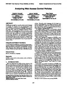
The key to ACL composition is the overlap of request types, because it implies interdependency between decisions taken by different decision functions. Let L1 = hF1 , C1 , δ1 i and L2 = hF2 , C2 , δ2 i be two ACLs that act in composition, e.g., suppose L2 is over L1 in the network stack. Then, every lower layer request shall match to some upper layer policy decision point, hence the upper layer coupling type C2 is included in the lower layer request type F1 . Furthermore, it may be the case that the two layers’ request types have some fields in common, that is F1 and F2 have a non empty intersection. Figure 1b depicts this situation, where the double hatched areas identify the overlap between layers. The union of the request types of L1 and L2 can then be thought as the request type of a new ACL L, that we are going to define as their composition. The decision function of L needs to depend both on δ1 and δ2 . If we assumed a boolean decision space, then we would expect every lower layer request ql that agrees with an upper layer request qu to yield a composite request that is allowed if and only if both ql and qu are allowed. In the following definition we generalize this intuition by substituting the logic conjunction by the greatest lower bound operator u. Definition 6 (ACL Composition): Given the ACLs L1 = hF1 , C1 , δ1 i and L2 = hF2 , C2 , δ2 i such that C2 ⊆ F1 and C1 ∩ F2 = ∅, their composition is the ACL L1 ⊗ L2 = hF1 ∪ F2 , C1 , δi, where δ is defined as follows: δ : Q(C1 ∪ F1 ∪ F2 ) → D

q 7→ δ1 (q|C1 ∪F1 ) u δ2 (q|C2 ∪F2 ).

(1)

As an example, we consider the composition Lc of ACLs La and Lb introduced in Section II. La ⊗ Lb = Lc = h{Is , Id , Ps , Pd , H, U} , {]} , δc i, where the graph of δc is represented in Table IV. For instance, the request h2.2.2.1, 1.1.1.1, 0, 80, acme.com, /private/i is authorized in Lc because La allows h2.2.2.1, 1.1.1.1, 0, 80i and Lb allows h2.2.2.1, acme.com, /private/i. However, the decision related to the request h3.3.3.3, 1.1.1.20, 0, 80, acme.com, /private/i is ⊥ because it is unknown whether any Web server is listening on the IP address 1.1.1.20. Given an ACL L = hF, C, δi, decomposition is the problem of finding ACLs L1 = hF1 , C1 , δ1 i and L2 = hF2 , C2 , δ2 i such that L1 ⊗ L2 = L. As Definition 6 defines the structure of the candidate decompositions, the problem amounts to compute δ1 and δ2 from δ. This means that, for every request q1 ∈ Q(F1 ∪ C1 ), we need the value of δ1 (q1 ) as a function of all the requests q ∈ Q(F ) such that q|F1 ∪C1 = q1 .

Is

Id

Ps

Pd

H

U

D

1.1.1.∗ 1.1.1.∗ 1.1.1.∗ 1.1.1.∗ 1.1.1.∗ 1.1.1.∗ 2.2.∗.∗ 2.2.2.∗ 2.2.3.∗ 3.3.∗.∗ 3.3.∗.∗\ 3.3.3.∗

1.1.1.1 1.1.1.1 1.1.1.1 1.1.1.1 1.1.1.1 1.1.1.∗\ 1.1.1.1 1.1.1.1 1.1.1.1 1.1.1.1 1.1.1.∗\ 1.1.1.1

∗ ∗ ∗ ∗ ∗ ∗ ∗ ∗ ∗ ∗

≤79 80 80 80 ≥81 ∗ 80 80 80 80

∗ acme.com acme.com beta.com ∗ ∗ acme.com acme.com beta.com ∗

∗ /public/∗ /private/∗ /∗ ∗ ∗ /public/∗ /private/∗ /∗ ∗

⊥ 1 1 1 ⊥ ⊥ 1 1 1 ⊥

1.1.1.1

∗

80

acme.com

/public/∗

1

...

0

In the case of a boolean decision space, the natural semantics we would like to assign to such an operation is that of projection. For instance, let δ : Q(F ) → B. Its projection on P ⊆ F would be π P (δ) : Q(P ) → B such that π P (δ)(q) = 1 if and only if δ(q 0 ) = 1 for at least one q 0 ∈ Q(F ), q 0 |F1 ∪C1 = q. Hence, π P (δ) would map each q to the logic disjunction of all such δ(q 0 ). In the next definition we generalize to larger decision spaces by replacing disjunction with least upper bound t. Definition 7 (Projection): The projection of a decision function δ : Q(F ) → D over the set of fields P ⊆ F is the decision function π P (δ) defined as follows:

π P (δ) : Q(P ) → D G q 7→

δ(q + x).

(2)

x∈Q(F \P )

As stated in the next proposition, decompositions obtained through projection are always the least permissive among those that preserve the composite decision function unchanged. Proposition 1 (Least Privilege Decomposition): Let L = hF1 ∪ F2 , C1 , δi such that L = hF1 , C1 , δ1 i ⊗ hF2 , C2 , δ2 i. Then, ∀q ∈ Q(Fi ∪ Ci ), π Fi ∪Ci (δ)(q) ≤ δi (q) for i ∈ {1, 2}. This result guarantees the least privilege principle for policy refactoring as stated in the introduction. We begin to see that the definitions of composition and decomposition can be suitable tools to tackle the refactoring problem. IV. C OMPACT R EPRESENTATION The request spaces we considered so far are, in general, infinite or very large in cardinality. This follows from the fact that each field can have either an infinite (e.g. URLs) or a very big (e.g. IP addresses) domain of values. In order to cope with this issue, in this section we introduce a finite and compact representation for generic request spaces and decision functions. We then show how (de)composition can be computed on instances of such a representation. Definition 8 (Field Descriptor): Given a request field f ∈ F, a field descriptor for f is a structure hΦf , J·Kf i where Φf is a language that allows to describe sets of elements in the domain of f and J·Kf : Φf → 2dom(f ) is an interpretation function that maps every sentence of the language to its extension, i.e., the subset of the field’s domain it describes.

TABLE V I NTEGERS R ANGE F IELD D ESCRIPTOR

Φ

Definition

Example

ϕ ::= ‘[’ n ‘:’ m ‘]’

ϕ1 = [0 : 100]

m ::= n | ∞

ϕ2 = [20 : ∞]

n ::= Integer

h‘[’ n1 ‘:’ m1 ‘]’,

∧

‘[’ n2 ‘:’ m2 ‘]’i 7→

‘[’ max(n1 , n2 ) ‘:’

min(m1 , m2 ) ‘]’

J·K

‘[’ n ‘:’ m ‘]’ 7→

{i | n ≤ i ≤ m}

ϕ3 = [200 : 1000] ϕ1 ∧ ϕ2 = [20 : 100]

ϕ1 ∧ ϕ3 = [200 : 100] Jϕ1 K = {0, 1, . . . , 100}

Algorithm 1 ACL Composition with DFD Input: L1 = hF1 , C1 , ∆1 i , L2 = hF2 , C2 , ∆2 i are ACLs. Output: L1 ⊗L2 1: W ← (F1 ∩ F2 ) ∪ C2 2: U ← (F1 ∪ C1 ) \ W 3: V ← (F2 ∪ C2 ) \ W 4: ∆ ← ∅ 5: for all hψ1 , d1 i ∈ ∆1 , hψ2 , d2 i ∈ ∆2 do 6: if Jψ1 |W ∧ ψ2 |W KW 6= ∅ then 7: ψ ← (ψ1 |W ∧ ψ2 |W ) + ψ1 |U + ψ2 |V 8: ∆ ← ∆ ∪ {hψ, d1 u d2 i} 9: end if 10: end for 11: return hF1 ∪ F2 , C1 , ∆i

Jϕ1 ∧ ϕ2 K = {20, 21, . . . , 100} Jϕ1 ∧ ϕ3 K = ∅

Furthermore, the descriptor language is closed under the intersection of sentences’ extensions, namely ∀ϕ1 , ϕ2 ∈ Φf , ∃ϕ3 ∈ Φf s.t. Jϕ3 Kf = Jϕ1 Kf ∩ Jϕ2 Kf . For every such combination we call ϕ3 the conjunction of ϕ1 , ϕ2 , written ϕ3 = ϕ1 ∧ ϕ2 . In Table V we provide an example field descriptor that allows to describe intervals of positive integers. A bounded interval is described by a pair of integers representing its minimum and maximum values; an unbounded one has its maximum value set to ∞. The conjunction of two intervals is the (potentially empty) interval ranging from the maximum of their lower boundaries to the minimum of their upper ones. This descriptor is already suitable for representing many of the fields introduced in Table I (i.e., Is , Id , Ps , Pd ). For fields associated with large or infinite domains of strings (such as U) we could analogously define a field descriptor where the sentences in Φ are arbitrary regular expressions, and their conjunction is the intersection of the corresponding automata. When we put together a collection of field descriptors, we obtain an object suitable to describe sets of requests. This is formalized in the following definition, which recasts Definitions 2 and 3 to the language of field descriptors. Definition 9 (Requests Descriptor): Let F be a set of fields and, for every field f ∈ F , let hΦf , J·Kf i be an associated field descriptor. We then define the requests descriptors space n on F = {fi }i=1 as the product of all the languages Φfi taken according to : Ψ(F ) = Φf1 × . . . × Φfn , fi  fj for i ≤ j. Every sequence ψ = hϕ1 , . . . , ϕn i ∈ Ψ(F ) is a Request Descriptor (RD) for the request space Q(F ). The concatenation ψ + ψ 0 and the projection ψ|P ⊆F from Definition 3 extend naturally to RDs. Moreover, if ψ = hϕ1 , . . . , ϕn i , ψ 0 = hϕ01 , . . . , ϕ0n i are RDs on Q(F ), we define their conjunction as ψ ∧ ψ 0 = hϕ1 ∧ ϕ01 , . . . , ϕn ∧ ϕ0n i. The extension of an a RD ψ, written JψKF , is the product of the extension of the sentences ϕi . Formally: JψKF = Jψ(f1 )Kf1 × . . . × Jψ(fn )Kfn , fi  fj for i ≤ j. Now, we can define a finite descriptor for decision functions. Definition 10 (Decision Function Descriptor): Given a set of fields F and a decision space D, a Decision Function Descriptor (DFD) is a finite relation ∆ ⊆ Ψ(F ) × D that

covers the entire request space Q(F ), that is such that [ {JψKF | hψ, ·i ∈ ∆} = Q(F ).

(3)

The decision function δ : Q(F ) → D is the extension of ∆, written δ = ext (∆), if the next statement holds: G δ(q) = {d | hψ, di ∈ ∆ ∧ q ∈ JψKF } , ∀q ∈ Q(F ). (4) Note that, as a consequence of (4), the condition (3) can be always fulfilled without altering the extension of the rest of the policy by adding a default RD to ∆ that (i) matches all the possible requests and (ii) is associated with the decision 0D . Moreover, whenever a concrete policy language features a deny by default semantics (as it is typically the case, e.g., for firewalls), the translation of such policies to DFD reduces to computing decisions for all the possible overlaps among rules within the policy. As discussed in Section VI the latter problem has been already extensively studied in literature on policy conflicts, hence it is left out in this paper. We now define two operations on DFDs that are consistent with the (de)composition of decision functions. Definition 11 (DFD Projection): The projection of a DFD ∆ over the set of fields P ⊆ F is the DFD π P (∆) = ∆0 such that: hψ, di ∈ ∆ ⇒ hψ|P , di ∈ ∆0 . (5) To see that Definition 11 is equivalent to the projection (Definition 7) of the DFD extension, it is sufficient to combine (4) with (5), that yields precisely (2). Algorithm 1 computes instead the composition (Definition 6) of ACLs whose decision function is described by a DFD. The correctness of the algorithm, as stated in Proposition 2, is ensured by showing that the extension of the output DFD is the same as the composition of the extension of the input DFDs. Proposition 2 (Correctness of Algorithm 1): Let the output of the algorithm be hF1 ∪ F2 , C1 , ∆i for input ACLs hF1 , C1 , ∆1 i and hF2 , C2 , ∆2 i. Then, hF1 , C1 , ext(∆1 )i ⊗ hF2 , C2 , ext(∆2 )i = hF1 ∪ F2 , C1 , ext(∆)i. Note how both Definition 11 and Algorithm 1 benefit from the choice of allowing the RDs in a DFD to overlap. In particular, we were able to define both operations without ever computing the disjunction or the complement of RDs

(resp. the union and the difference of their extensions). This is convenient as the Cartesian product distributes with respect to intersection, but not to union and difference. Hence, as argued in [8], a number of RDs that grows linearly with the dimension of the product would be necessary to represent each binary union or difference. In order to perform refactoring, we need to determine whether a decomposition is possible. This is equivalent to check if a decision function, once projected and composed back, equals itself. As different DFDs can have the same extension, this translates into testing the equivalence of hF1 ∪ F2 , C1 , ∆i with hF1 , C1 , π F1 ∪C1 (∆)i ⊗ hF2 , C2 , π F2 ∪C2 (∆)i, which means to compare the (possibly infinite) extensions of their DFDs. In the next section we deal with this issue by developing an alternative criterion to test decomposability. V. R EFACTORING Through decomposition, we aim at factorizing the complexity of some layer’s policy into simpler ones. This means that the request type of any of the decomposed layers shall be a strict subset of the one of the original (composite) layer. The next result shows that it is not guaranteed that such a decomposition exists for a generic access control layer. Proposition 3: Given an ACL L = hF1 ∪ F2 , C1 , δi it is not always possible to find two ACLs hF1 , C1 , δ1 i, hF2 , C2 , δ2 i that decompose L with F2 6⊆ F1 . Sketch of the proof: Assume that such a decomposition exists. Let q1 , q2 , q3 ∈ Q(F1 ∪ F2 ∪ C1 ) such that q1 6= q2 6= q3 and q1 |C2 ∪F2 = q2 |C2 ∪F2 and q2 |C1 ∪F1 = q3 |C1 ∪F1 . The assumption that F2 6⊆ F1 is crucial, otherwise q2 = q3 . One choses δ such that δ(q1 ) 6= 0D ∧ δ(q2 ) = 0D ∧ δ(q3 ) 6= 0D to obtain, according to (1), a contradiction. The counterexample shown in the last proof captures the essence of non-decomposability. Consider, for instance, the decision function δc (Table IV) and let q1 = h2.2.2.1, 1.1.1.1, 0, 80, acme.com, /private/i, q2 = h2.2.3.1, 1.1.1.1, 0, 80, acme.com, /private/i and q3 = h2.2.3.1, 1.1.1.1, 0, 80, beta.com, /i. Note that, in case C1 ∪ F1 = {Is , Id , Ps , Pd } and C2 ∪ F2 = {Id , Pd , H, U}, we have indeed a contradiction. In fact, as δ(q2 ) = 0, we need either δ1 (h2.2.3.1, 1.1.1.1, 0, 80i) = δ1 (x) = 0 or δ2 (hacme.com, /private/i) = δ2 (y) = 0. On the other hand, as δ(q1 ) = δ(q3 ) = 1, both δ1 (x) = 1 and δ2 (y) = 1 must hold. Intuitively, we see that in order to have decomposability, the decisions associated to requests that satisfy a specific inter-field dependency cannot be independent one from another. The next definition formalizes this intuition. Definition 12 (Inter-Field Dependency): For W and V non-empty and disjoint subsets of F , we say that a decision function δ satisfies the Inter-Field Dependency (IFD) condition W → → V , written δ |= W → → V , if and only if ∀q, q 0 ∈ Q(F ), q|W = q 0 |W ⇒ δ(q) u δ(q 0 ) = δ(q|F \V + q 0 |V ) u δ(q|V + q 0 |F \V ). We are now ready to state the main result of this section: IFDs precisely characterize when an ACL can be decomposed by projections without loss.

Algorithm 2 DFD Partition Input: ∆ ⊆ Ψ(F ) × D. Input: X ⊆ F . Output: PARTITION(∆, X) 1: Y ← F \ X 2: P ← ∅ 3: for all hψ, di ∈ ∆ do 4: P ← P ∪ {ψ|X , {hψ|Y , di}} 5: end for 6: while ∃ hψ1 , ∆1 i , hψ2 , ∆2 i ∈ P s.t. Jψ1 ∧ ψ2 KX 6= ∅ do 7: P ← P \ {hψ1 , ∆1 i , hψ2 , ∆2 i} 8: P ← P ∪ {hψ1 ∧ ψ2 , ∆1 ∪ ∆2 i} 9: for all ψ1\2 ∈ D IFF(ψ1 , ψ2 ), ψ2\1 ∈ D IFF(ψ2 , ψ1 ) do 10: if Jψ1\2 KX 6=

∅ then  11: P ← P ∪ ψ1\2 , ∆1 12: end if 13: if Jψ2\1 KX 6=

∅ then  14: P ← P ∪ ψ2\1 , ∆2 15: end if 16: end for 17: end while 18: return P

Algorithm 3 Inter-Field Dependency check on DFD Input: ∆ ⊆ Ψ(F ) × D. Input: W → → V , with W, V ∈ 2F \ {∅}, W ∩ V = ∅. Output: true/false 1: U ← F \ (W ∪ V ) 2: for all hψW , ∆W i ∈ PARTITION(∆, W ) do 3: PU , PV ← ∅ 4: for all hψU , ∆U i ∈ PARTITION(∆W , U ) do 5: PU ← PU ∪ {ψU } 6: PV [ψU ] ← PARTITION(∆U , V ) 7: end for 0 ∈ P do 8: for all ψU , ψU U

0  0 ] do 9: for all hψVF, ∆V i ∈ P[ψU ], ψV , ∆0V ∈ P[ψU F 10: d1 ← {d | h·, di ∈ ∆ } u d | h·, di ∈ ∆0V V 

000 000  00 00 0 11: for all ψV , ∆V ∈ P[ψU ], ψV , ∆V ∈ P[ψU ] do 0 ∧ ψ 00 K 6= ∅ ∧ Jψ ∧ ψ 000 K 6= ∅ then 12: if JψV V VFV FV V 13: d2 ← d | h·, di ∈ ∆00 d | h·, di ∈ ∆000 V u V 14: if d1 6= d2 then 15: return false 16: end if 17: end if 18: end for 19: end for 20: end for 21: end for 22: return true

Theorem 4 (Decomposability): Given a generic ACL L = hF1 ∪ F2 , C1 , δi, the following are equivalent: • L = hF1 , C1 , π F1 ∪C1 (δ)i ⊗ hF2 , C2 , π F2 ∪C2 (δ)i • δ |= (F1 ∩ F2 ) ∪ C2 → → (F2 \ F1 ). Theorem 4 gives an alternative criterion to test the decomposability of an ACL: we need to check if its decision function satisfies the IFD (F1 ∩ F2 ) ∪ C2 → → (F2 \ F1 ), for the subsets F1 , F2 , C2 of its request type (with C2 ⊆ F1 ) that represent the new layers’ layout we want to find a policy for. IFDs are particularly interesting because they are constraints on the internal structure of the decision function that we can as well check on any corresponding DFDs. Algorithm 3 computes this check and the next proposition ensures its correctness. Proposition 5 (Correctness of Algorithm 3): Let ∆ ⊆ Ψ(F ) × D be a DFD, δ = ext (∆) its extension

and W, V two non-empty and disjoint subsets of F . Then, ∆ |= W → → V ⇔ δ |= W → → V. The key ideas underlying Algorithm 3 are as follows: First, we refactor the RDs contained in ∆ to make them partition the entire request space (lines 2–7) such that every request matches exactly one RD ψW + ψU + ψV . Second, for every 0 ψW , we consider all the pairs ψU , ψU and ψV , ψV0 (lines 8, 9) and we compute the greatest lower bound of the decisions associated with all the pairs of requests matching respectively 0 ψW +ψU +ψV and ψW +ψU +ψV0 (line 10). We finally check if the latter equals the greatest lower bound of all the pairs of 0 requests matching ψW +ψU +ψV0 and ψW +ψU +ψV (lines 11– 18). To do the request space partition, we use iteratively the procedure defined by Algorithm 2 that computes a closure w.r.t. intersection and difference for the portion of the RDs concerning the subset of fields X. Note that here, unlike for previous algorithms, we need to compute the set of RDs describing the difference between two given RDs, formally S D IFF(ψ1 , ψ2 ) = {ψi∗ } s.t. {Jψi∗ KF } = Jψ1 KF \ Jψ2 KF . This is generally possible for the RDs composed of the field descriptors considered in this paper (e.g., intervals of integers). Given any ACL we can now first test for decomposability by the means of Algorithm 3 and then, in case of success, project (Definition 11) to obtain the desired decomposition. Consider, for example, the ACL L3 = h{Is , Id , Ps , Pd , H, U}, {]}, δc i that was introduced in Section III. As it is the result of the composition of ACLs La = h{Is , Id , Ps , Pd } , {]} , δa i and Lb = h{Is , H, U} , {Id , Pd } , δb i, we naturally expect it to be decomposable with respect to their same structure. The reader can check, by inspecting Table IV, that indeed δc |= {Is , Id , Pd } → → {H, U}. Hence, if we name 0 = {I , I , P , P } , {]} , π {Is ,Id ,Ps,Pd } (δc ) and L0b = L s d s d a

{Is , H, U} , {Id , Pd } , π {Is ,Id ,Pd ,H,U} (δc ) , we know by Theorem 4 that L3 = L0a ⊗ L0b . This is an example of refactoring that keeps the request type unchanged. Table VI represents the decision function π {Is ,Id ,Ps ,Pd } (δc ). Notice that it is not exactly equal to the original decision function δa of the ACL La (cf. Table II). In particular, it is never more permissive than the original; on the other hand it is, where possible and according to the least privilege principle, more restrictive. For instance, requests coming from the 3.3.3.0/24 IP network and directed to 1.1.1.1, which were allowed by the original policy, are denied by the refactored version. This is consistent with the fact that such requests were anyway already denied in Lb (cf. Table III). On the other hand, the decisions for all requests having source within 3.3.0.0/24 and directed to the rest of the 1.1.1.0/24 network, are refactored to ⊥. This is a consequence of assuming partial knowledge of the Lb policy. Since additional information is required to decide on the usefulness of those permissions, the choice is left to the user who can either trust the original policy, i.e., change ⊥ to 1, or follow a more restrictive approach and change ⊥ to 0. Let us now try to refactor La , Lb to a pair of ACLs that have smaller request types. Suppose, for instance, to substitute the WS Web server of our scenario with one that does not discriminate requests on the basis of the IP

TABLE VI E XAMPLE P ROJECTION {Is ,Id ,Ps ,Pd } (δc )

π

Is

Id

Ps

Pd

D

1.1.1.∗ 1.1.1.∗ 1.1.1.∗ 1.1.1.∗ 2.2.∗.∗ 3.3.∗.∗\ 3.3.3.∗ 3.3.∗.∗

1.1.1.1 1.1.1.1 1.1.1.1 1.1.1.∗\ 1.1.1.1 1.1.1.1 1.1.1.1 1.1.1.∗\ 1.1.1.1 ...

∗ ∗ ∗ ∗ ∗ ∗ ∗

≤79 80 ≥ 81 ∗ 80 80 80

⊥ 1 ⊥ ⊥ 1 1 ⊥ 0

source address; this means that the field Is does not belong any more to the request type of L00b . We know, however, that such a decomposition is not possible, as δc 6|= {Id , Pd } → → {H, U}. See, as proof, the counterexample given earlier in this section, that clearly violates the condition given in Definition 12. Had all the requests with H = acme.com in δc been mapped to 0, the IFD would have been instead satisfied. In such a case we would have had a rafactoring with a change in request types that simplified the decision function δb . VI. R ELATED W ORK The pioneering work of Moffett and Sloman [9] has opened a large avenue for research on policy conflict analysis in distributed systems and has been refined, classified and formalized in the network-level security field. For instance, AlShaer et al. [10] or Basile et al. [8] have proposed techniques and algorithms to automatically discover and manage inconsistencies between firewall rule sets. One of the key points of these techniques is to turn rule sets into some canonical structure (e.g., ordered binary decision diagram [10], intersection closed semi-lattice of subsets [8]): An intermediate policy representation on which analysis and discovery is performed. Although this paper does not focus on inconsistencies, it shares the abstract definition of devices and the ideas behind composition of policies to capture and analyze interactions between different layers. Related work on network-level analysis may complete our approach by providing means to deal with interactions between firewalls. There exists a substantial body of work on combination of policies not limited to firewalls. Notably, several logical and algebraic approaches for composing and unifying access control policies have been proposed quite recently [7], [5], [6]. Different algebraic varieties have been used to combine rich decision spaces, for instance, D-algebras [7], Belnap bilattices [6] or XACML tailored logic [5]. One of the goals is to provide mathematical foundations to the expressive XACML access control language and its many resolution strategies. The algebraic structure chosen here for decision space is motivated by previous work which have shown the need for expressive ones. However, the goal is not to capture resolution strategies but to find a structure both expressive enough and sufficient to define a decomposition with good properties. The use of an expressive common pivot model like XACML, logical frameworks or subject-target-condition rules [11] is very interesting. However, this paper chooses

a different perspective by sticking as closely as possible to the original policies. Algorithms 1 and 3 carry computation directly on original policies, with minimal prior normalization. Our approach has a strong connection to the policy refinement problem [12], [13], [11]. The key difference is that we start from interdependent concrete policies and we provide a device oriented decomposition instead of starting from high level requirements which are ultimately refined into operational policies. The refactoring problem studied in this paper is bottom-up: The global policy is nothing but the composition of all devices interacting along the network stack. By contrast, the policy refinement problem is clearly top-down. Finally, the definition of access control layer is quite close to that of abstract access control systems [14], [15], [4]. The first two references formally compare the expressiveness of access control models with respect to the set of decision functions they can produce. Interest is not brought on the state but on the model itself, whereas we focus on the first. For the last, a set of desirable properties of abstract access control systems is identified. The question whether our decomposition technique still applies in their case is left for future work. VII. C ONCLUSION This paper proposes a relational oriented approach for access control policies decomposition. The key concept that captures decomposability is the inter-field dependency condition given in Section V from which an algorithm for decomposability is derived. This algorithm works directly on a relational representation of access control policies. Relational database users may have recognized the syntactical resemblance between W → → V of Definition 12 and so-called MultiValued Dependencies (MVD) introduced in [3]. The two concepts are related in the fact that Theorem 1 of [3], linking lossless decomposition of a relation and MVDs, is a specific instance of Theorem 4 of this paper, when the decision space is reduced to the two-elements boolean algebra. We argue that the relational databases machinery can be fruitfully mapped to solve policies management problems. As ongoing and future work, we describe two such problems for which techniques borrowed from the database community could be of great interest. The first problem is about repairs. Assume an access control policy over several fields cannot be decomposed into independent sub-policies: Is there any canonical or best way to update the policy such that it will become decomposable? Applying the many results for the repair problems (e.g., see [16]) to policies is not without difficulties. Basically, one has to generalize the relational framework to be able to capture generic definition of access control systems and thus has to provide new results inspired from classical ones, as we have done for MVD in some sense. Moreover, one has to find repair semantics meaningful from the security point of view. Standard repair semantics are repair via insertions, deletions or updates [17]. It is interesting to study how these semantics apply to policy decomposition, the last one in particular.

The second problem is about the mining of dependencies. In the classical setting of database normalization, the set of dependencies is known in advance and one tries to provide the best structure fitting with the given constraints, as it is done in this paper. The data-mining perspective reverses the approach: The goal is to discover new dependencies by revealing the internal structure of relations. Savnik and Flach have provided an efficient algorithm to discover MVD [18], we envision to apply their techniques to reverse engineer large policies. The idea is to find some “best set of simplest access control systems” with the same authorized queries. ACKNOWLEDGMENT This work was partially supported by the FP7-ICT-2009.1.4 Project PoSecCo (no. 257129, www.posecco.eu). R EFERENCES [1] 7Safe and the University of Bedfordshire, “Uk security breach investigations report 2010,” http://www.7safe.com/breach report/Breach report 2010.pdf, 2010. [2] E. Al-Shaer, “Security automation research: Challenges and future directions,” IAnewsletter, vol. 14, no. 4, pp. 14–18, 2011. [3] R. Fagin, “Multivalued dependencies and a new normal form for relational databases,” ACM Trans. Database Syst., vol. 2, no. 3, pp. 262–278, Sep. 1977. [4] J. Crampton and C. Morisset, “Towards a generic formal framework for access control systems,” CoRR, vol. abs/1204.2342, 2012. [5] C. D. P. K. Ramli, H. R. Nielson, and F. Nielson, “The logic of xacml,” in FACS, 2011, pp. 205–222. [6] G. Bruns and M. Huth, “Access control via belnap logic: Intuitive, expressive, and analyzable policy composition,” ACM Trans. Inf. Syst. Secur., vol. 14, no. 1, pp. 9:1–9:27, Jun. 2011. [7] Q. Ni, E. Bertino, and J. Lobo, “D-algebra for composing access control policy decisions,” in ASIACCS ’09 . New York, NY, USA: ACM, 2009, pp. 298–309. [8] C. Basile, A. Cappadonia, and A. Lioy, “Network-level access control policy analysis and transformation,” Networking, IEEE/ACM Transactions on, vol. 20, no. 4, pp. 985–998, 2012. [9] J. D. Moffett and M. S. Sloman, “Policy conflict analysis in distributed system management,” Journal of Organizational Computing, vol. 4, pp. 1–22, 1994. [10] E. Al-Shaer, H. Hamed, R. Boutaba, and M. Hasan, “Conflict classification and analysis of distributed firewall policies,” IEEE Journal on Selected Areas in Communications, vol. 23(10), pp. 2069–2084, 2005. [11] H. Zhao, J. Lobo, A. Roy, and S. M. Bellovin, “Policy refinement of network services for MANETs,” in The 12th IFIP/IEEE International Symposium on Integrated Network Management (IM 2011), Dublin, Ireland, May 2011, to appear. [12] R. Craven, J. Lobo, E. C. Lupu, A. Russo, and M. Sloman, “Decomposition techniques for policy refinement,” in CNSM, 2010, pp. 72–79. [13] R. Craven, J. Lobo, E. Lupu, A. Russo, and M. Sloman, “Policy refinement: Decomposition and operationalization for dynamic domains,” in CNSM, 2011, pp. 1–9. [14] M. V. Tripunitara and N. Li, “A theory for comparing the expressive power of access control models,” J. Comput. Secur., vol. 15, no. 2, pp. 231–272, 2007. [15] L. Habib, M. Jaume, and C. Morisset, “Formal definition and comparison of access control models,” Journal of Information Assurance and Security, vol. 4, pp. 372–378, 2009. [16] L. E. Bertossi, Database Repairing and Consistent Query Answering, ser. Synthesis Lectures on Data Management. Morgan & Claypool Publishers, 2011. [17] J. Wijsen, “Database repairing using updates,” ACM Trans. Database Syst., vol. 30, no. 3, pp. 722–768, Sep. 2005. [18] I. Savnik and P. A. Flach, “Discovery of multivalued dependencies from relations,” Intell. Data Anal., vol. 4, no. 3,4, pp. 195–211, 2000.

F F1 C1

F2

C2

U W V

Fig. 2.

Request Types Partition

A PPENDIX Note to the reviewers: this appendix is provided for the sake of completeness and will be not part of the camera-ready version, if any. Lemma 6: Let hF1 ∪ F2 , C1 , δi = hF1 , C1 , δ1 i ⊗ hF2 , C2 , δ2 i, W = (F1 ∩ F2 ) ∪ C2 , U = ((F1 \ F2 ) \ C2 ) ∪ C1 and V = F2 \ F1 . Then, {U, V, W } is a partition of (F1 ∪ C1 ∪ F2 ). Proof: Recall that Fi ∩ Ci = ∅, i ∈ {1, 2} (Definition 4) and that C2 ⊆ F1 , F2 ∩ C1 = ∅ (Definition 6). We then have the following equalities, which can be easily verified by inspection of Figure 2: U ∪ W = ((F1 \ F2 ) \ C2 ) ∪ C1 ∪ (F1 ∩ F2 ) ∪ C2 = = (F1 \ F2 ) ∪ (F1 ∩ F2 ) ∪ C1 = F1 ∪ C1 U ∩ W = (((F1 \ F2 ) \ C2 ) ∪ C1 ) ∩ ((F1 ∩ F2 ) ∪ C2 ) = ∅ V ∪ W = (F2 \ F1 ) ∪ (F1 ∩ F2 ) ∪ C2 = F2 ∪ C2 V ∩ W = (F2 \ F1 ) ∩ ((F1 ∩ F2 ) ∪ C2 ) = ∅ U ∩ V = (((F1 \ F2 ) \ C2 ) ∪ C1 ) ∩ (F2 \ F1 ) = ∅ U ∪ V ∪ W = (F1 ∪ C1 ) ∪ (F2 ∪ C2 ) = F1 ∪ C1 ∪ F2 .

Lemma 7: Let L be a finite bounded distributive lattice and f : X → L, g : Y → L two generic functions having L as codomain. Then the following holds true: G G G f (x) u g(y) = f (x) u g(y). (6) x∈X

y∈Y

x∈X∧y∈Y

F Proof: As L Fis finite and because of lattices’ idempotence, F f (x) = {l ∈ LF| ∃x ∈ X, l = f (x)} = Lf ⊆ L. x∈X F Likewise y∈Y g(y) = Lg ⊆ L. By applying the distributive law of t with respect to u n times, where n = |Lf |×|Lg | we obtain: G G G G G f (x) u g(y) = lu l0 = l u l0 . x∈X

y∈Y

l∈Lf

l∈Lg

l∈Lf ∧ l0 ∈Lg

As there are up to n different pairs hl, l0 i, by idempotence we conclude the thesis. Proof of Proposition 1: Let L = hF1 ∪ F2 , C1 , δi such that L = hF1 , C1 , δ1 i ⊗ hF2 , C2 , δ2 i. By Lemma 6, sets W = (F1 ∩ F2 ) ∪ C2 , U = ((F1 \ F2 ) \ C2 ) ∪ C1 and V = F2 \ F1 partition F . Moreover F1 ∪ C1 = W ∪ U (resp. F2 ∪ C2 = W ∪ V ).

By combining the definitions of projection (Definition 7) and composition (Definition 6) and using the distributive law we obtain, ∀q = wu ∈ Q(F1 ∪ C1 ) = Q(W ∪ U ),

π W ∪U (δ)(wu) =

G

δ(wuv) =

v∈Q(V )

G

δ1 (wu) u δ2 (wv)

v∈Q(V )

= δ1 (wu) u

G

δ2 (wv) ≤ δ1 (wu).

v∈Q(V )

Likewise we have, ∀q 0 = wv ∈ Q(F2 ∪ C2 ) = Q(W ∪ V ), π W ∪V (δ)(wv) ≤ δ2 (wv). Proof of Proposition 3: Let L = hF1 ∪ F2 , C1 , δi, where F1 , F2 , C1 ∈ 2F \ {∅} and assume that there exist L1 = hF1 , C1 , δ1 i and L2 = hF2 , C2 , δ2 i such that L = L1 ⊗ L2 (hence C2 ⊆ F1 ) and F2 6⊆ F1 . Let F = F1 ∪ C1 ∪ F2 . By Lemma 6, sets W = (F1 ∩ F2 ) ∪ C2 , U = ((F1 \ F2 ) \ C2 ) ∪ C1 and V = F2 \ F1 partition F . Since we assumed F2 6⊆ F1 and sets F1 , F2 are not empty by hypothesis, it must hold that U and V are not empty either. Hence, ∃ u1 , u2 ∈ Q(U ) ∃ v1 , v2 ∈ Q(V ) such that u1 6= u2 ∧ v1 6= v2 . Moreover, as W, U, V partition F , there exist q1 , q2 , q3 ∈ Q(W ∪ U ∪ V ) = Q(F ) such that: q1 = wu1 v1 q2 = wu2 v1 q3 = wu2 v2 . Assume now δ(q1 ) 6= 0D ∧ δ(q2 ) = 0D ∧ δ(q3 ) 6= 0D that, according to Definition 6, entails the following contradiction:   δ (q | ) = δ1 (wu2 ) 6= 0D   1 3 C1 ∪F1 δ2 (q1 |C2 ∪F2 ) = δ2 (wv1 ) 6= 0D   δ (q | 1 2 C1 ∪F1 ) = δ1 (wu2 ) = 0D ∨ δ2 (q2 |C2 ∪F2 ) = δ2 (wv1 ) = 0D .

Proof of Proposition 4: As stated in Lemma 6, it is possible to partition the decision space of δ in the following three sets of fields: W = (F1 ∩F2 )∪C2 , U = ((F1 \F2 )\C2 )∪ C1 and V = F2 \ F1 . A generic request q in such a request space can then be expressed as the concatenation of sequences w ∈ Q(W ), u ∈ Q(U ) and v ∈ Q(V ), i.e., q = wuv. ⇐. For the if direction we assume δ |= W → → V and we show that ∀q ∈ Q(F ), π F1 ∪C1 (δ)(q|F1 ∪C1 ) u π F2 ∪C2 (δ)(q|F2 ∪C2 ) = δ(q). First, notice that, as δ |= W → → V , according to Definition 12 the following is true ∀w ∈ Q(W ), u, u0 ∈ Q(U ), v, v 0 ∈ Q(V ): δ(wuv) u δ(wu0 v 0 ) = δ(wuv 0 ) u δ(wu0 v).

(7)

We now have the following sequence of equalities (the passages marked by distr. and abs. hold respectively by distribu-

tive and absorption lattice laws).

π W ∪U (δ)(wu) u π W ∪V (δ)(wv) 



G

=  0



δ(wuv 0 ) u 

v ∈Q(V )

G



δ(wu0 v)

by (2)

0

u ∈Q(U )

= δ(wuv) t

G

= δ(wuv) t

G

= δ(wuv) t

G

= δ(wuv) t

G

0

δ(wuv ) u δ(wuv) t

v 0 ∈Q(V )\{v}

G

By repeating the same reasoning on δ(wu1 v2 ), δ(wu2 v1 ), and δ(wu2 v2 ) we conclude   δ(wu1 v2 ) u δ(wu2 v1 ) ≤ δ(wu1 v1 )     δ(wu1 v2 ) u δ(wu2 v1 ) ≤ δ(wu2 v2 )  δ(wu1 v1 ) u δ(wu2 v2 ) ≤ δ(wu1 v2 )     δ(wu v ) u δ(wu v ) ≤ δ(wu v ), 1 1 2 2 2 1

0

δ(wu v)

u0 ∈Q(U )\{u}

(distr.)

that, as x ≤ y ∧ z ≤ w ⇒ x u z ≤ y u w, yields ( δ(wu1 v2 ) u δ(wu2 v1 ) ≤ δ(wu1 v1 ) u δ(wu2 v2 )

δ(wuv 0 ) u δ(wu0 v)

by (6)

δ(wu1 v1 ) u δ(wu2 v2 ) ≤ δ(wu1 v2 ) u δ(wu2 v1 ).

δ(wuv) u δ(wu0 v 0 )

by (7)

δ(wuv 0 ) u

v 0 ∈Q(V )\{v}

G

δ(wu0 v)

u0 ∈Q(U )\{u}

u0 ∈Q(U )\{u} v 0 ∈Q(V )\{v}

u0 ∈Q(U )\{u} v 0 ∈Q(V )\{v}

  G = δ(wuv) t δ(wuv) u δ(wu0 v 0 )

(distr.)

By antisymmetry, the latter entails δ(wu1 v1 ) u δ(wu2 v2 ) = δ(wu1 v2 ) u δ(wu2 v1 ), in contradiction with (9). Proof of Proposition 2: Let hF1 ∪ F2 , C1 , ∆i = hF1 , C1 , ∆1 i ⊗ hF2 , C2 , ∆2 i and hF1 ∪ F2 , C1 , δi = hF1 , C1 , δ1 i ⊗ hF2 , C2 , δ2 i . We need to show that

u0 ∈Q(U )\{u} v 0 ∈Q(V )\{v}

= δ(wuv).

(abs.)

⇒. For the only if direction we reason by contradiction. Assume ∀q ∈ Q(F )

π F ∪C 1

1

(δ)(q|F1 ∪C1 ) u π F2 ∪C2 (δ)(q|F2 ∪C2 ) = δ(q),

(8)

and δ 6|= W → → V . For instance, let δ(wu1 v1 ) u δ(wu2 v2 ) 6= δ(wu1 v2 ) u δ(wu2 v1 ),

(9)

for some w ∈ Q(W ), u1 , u2 ∈ Q(U ), v1 , v2 ∈ Q(V ). We know, from the first half of the proof, that we can rewrite (8) as G δ(wu1 v1 ) = δ(wu1 v1 ) t δ(wu1 v 0 ) u δ(wu0 v1 ). u0 ∈Q(U )\{u1 } v 0 ∈Q(V )\{v1 }

Now we take the greatest lower bound of the expression δ(wu1 v2 ) u δ(wu2 v1 ) with both sides of the equality. Then we recognize that the same expression is always a factor of the series of least upper bound operations. This allows us to cancel out the series by absorption: δ(wu1 v1 ) u δ(wu1 v2 ) u δ(wu2 v1 )

= δ(wu1 v2 ) u δ(wu2 v1 )u   G δ(wu1 v1 ) t δ(wu1 v 0 ) u δ(wu0 v1 ) u0 ∈Q(U )\{u1 } v 0 ∈Q(V )\{v1 }

= δ(wu1 v2 ) u δ(wu2 v1 )u  δ(wu1 v1 ) t δ(wu1 v2 ) u δ(wu2 v1 )t  G δ(wu1 v 0 ) u δ(wu0 v1 )

u0 v 0 ∈Q(U \{u1 }∪V \{v1 })\ {u2 v2 }

= δ(wu1 v2 ) u δ(wu2 v1 ); thus δ(wu1 v2 ) u δ(wu2 v1 ) ≤ δ(wu1 v1 ).

(10)

δ1 = ext (∆1 ) ∧ δ2 = ext (∆2 ) ⇒ δ = ext (∆) . Let us denote W ∪ U ∪ V = F . Let wu ∈ Q(W ∪ U ) and wv ∈ Q(W ∪ V ). Then consider all the pairs hψ1 , d1 i ∈ ∆1 and hψ2 , d2 i ∈ ∆2 such that wu ∈ Jψ1 KW ∪U ∧ wv ∈ Jψ2 KW ∪V . Since all such ψ1 , ψ2 guarantee w ∈ Jψ1 |W ∧ ψ2 |W KW , they surely fulfill the condition of line 6. Hence, by lines 7 and 8, there exists hψ, d1 u d2 i ∈ ∆ such that wuv ∈ JψKF . We thus have the following result: hψ1 , d1 i ∈ ∆1 ∧ wu ∈ Jψ1 KW ∪U ∧ hψ2 , d2 i ∈ ∆2 ∧

wv ∈ Jψ2 KW ∪V ⇔ hψ, d1 u d2 i ∈ ∆ ∧ wuv ∈ JψKF .

(11)

We can now prove our thesis:

∀wuv ∈ Q(F ), δ(wuv) = δ1 (wu) u δ2 (wv)

= ext (∆1 ) u ext (∆2 ) G = {d1 | hψ1 , d1 i ∈ ∆1 ∧ wu ∈ Jψ1 KW ∪U } u G {d2 | hψ2 , d2 i ∈ ∆2 ∧ wv ∈ Jψ2 KW ∪V } G = {d1 u d2 | hψ1 , d1 i ∈ ∆1 ∧ wu ∈ Jψ1 KW ∪U ∧ hψ2 , d2 i ∈ ∆2 ∧ wv ∈ Jψ2 KW ∪V } G = {d | hψ, di ∈ ∆ ∧ wuv ∈ JψKF } .

(Hyp)

by (4)

by (6) by (11)

Hence, by (4), we conclude δ = ext (∆). Lemma 8: Let ∆ ⊆ Ψ(F ) × D and X ⊆ F . Then, ∀q ∈ Q(F ), ∃! hψX , ∆X i ∈ PARTITION(∆, X) s.t. q|X ∈ JψX KX

(12)

ext(∆)(q) = ext(∆X )(q|F \X )

(13)

and Proof: The first result (12) follows by observing that the main loop of Algorithm 2 removes all the possible overlaps among the X-projection of the RDs in ∆. Hence, at most one ψX will exist that matches every possible q|X . More strongly, as the DFD covers the entire request space (cf. (3)), exactly

TABLE VII PARTITIONED ∆ PARTITION(∆jU , V )

PARTITION(∆iW , U )

PARTITION(∆, W )

hψU , ∆U i hψW , ∆W i



0 ψU , ∆0U



... ...

...

hψ , ∆ = {d1 , . . . , dn }i

00V 00V   00 ψV , ∆V = d00 1 , . . . , dm ...

0   ψ , ∆0V = d01 , . . . , d0l

000V 000  000  000 ψV , ∆V = d1 . . . , dk ... ... ...

one such q|X must exist. The second result (13) follows by substituting the definition of DFD extension (4). Proof of Proposition 5: ⇐. We obtain the first half by contraposition. Assume that Algorithm 3 returns false (Line 15). 0 Hence, there exist hψW , ∆W i , hψU , ∆U i , hψU , ∆0U i , 000 000 00 00 0 0 hψV , ∆V i , hψV , ∆V i , hψV , ∆V i , hψV , ∆U i such that:  hψW , ∆W i ∈ PARTITION(∆, W )      0 hψU , ∆U i , hψU , ∆0U i ∈ PARTITION(∆W , U )

d∈∆V

G d0 ∈∆0V

d0 6=

G d00 ∈∆00 V

d00 u

G

d000 .

(14)

(15)

d000 ∈∆000 V

Note that for all hψ, di ∈ ∆V (and likewise for ∆0V , ∆00V , ∆000 V ), ψ must equal the empty sequence hi. This is a consequence of partitioning ∆U ⊆ Ψ(V ) × D (resp. ∆0U ) on V . For the sake of clarity, we abuse notation and simply write d for hhi , di. According to (4), we can then rewrite (15) as: ext(∆V )(hi) u ext(∆0V )(hi) 6= ext(∆00V )(hi) u ext(∆000 V )(hi). (16) The partitions of ∆ are represented in Table VII. Because of (12) and (14) we can choose q, q 0 , q 00 , q 000 ∈ Q(W ∪ U ∪ V ) such that:   q|W , q 0 |W , q 00 |W , q 000 |W ∈ JψW KW       q| , q 00 |U ∈ JψU KU   U 0 q 0 |U , q 000 |U ∈ JψU KU    000  q|V , q |V ∈ JψV ∧ ψV000 KV     q 0 | , q 00 | ∈ Jψ 0 ∧ ψ 00 K V V V V V

V

V

ext(∆)(q) u ext(∆)(q 0 ) 6= ext(∆)(q 00 ) u ext(∆)(q 000 ). (17)

and (Lines 10, 13 and 14): du

V

and

and (Line 12):

G

that allows to rewrite (16) as ext(∆)(q) u ext(∆)(q 0 ) 6= ext(∆)(q 00 ) u ext(∆)(q 000 ), which, by Definition 12, is equivalent to ext(∆) 6|= W → →V. ⇒. For the second half, we reason again by contraposition. Assume ext(∆) 6|= W → → V . Then, there exist q, q 0 , q 00 , q 000 ∈ Q(W ∪ U ∪ V ) such that:  q|W = q 0 |W = q 00 |W = q 000 |W    q|U = q 00 |U ∧ q 0 |U = q 000 |U   q| = q 000 | ∧ q 0 | = q 00 | V

 hψV , ∆V i , hψV00 , ∆00V i ∈ PARTITION(∆U , V )     hψ 0 , ∆0 i , hψ 000 , ∆000 i ∈ PARTITION(∆0 , V ) V V V V U

JψV0 ∧ ψV00 KV 6= ∅ ∧ JψV ∧ ψV000 KV 6= ∅

moreover, as a consequence of (13), we have:   ext(∆)(q) = ext(∆W )(q|U ∪V ) = ext(∆U )(q|U ∪V |V )     = ext(∆V )(q|U ∪V |V |∅ ) = ext(∆V )(hi)       ext(∆)(q 0 ) = ext(∆W )(q 0 |U ∪V ) = ext(∆0U )(q 0 |U ∪V |V )      = ext(∆0 )(q 0 |U ∪V |V |∅ ) = ext(∆0 )(hi) V V 00 00  ext(∆)(q ) = ext(∆W )(q |U ∪V ) = ext(∆U )(q 00 |U ∪V |V )       = ext(∆00V )(q 00 |U ∪V |V |∅ ) = ext(∆00V )(hi)       ext(∆)(q 000 ) = ext(∆W )(q 000 |U ∪V ) = ext(∆0U )(q 000 |U ∪V |V )     000 000 = ext(∆000 V )(q |U ∪V |V |∅ ) = ext(∆V )(hi)

By (12) then, there is a unique hψW , ∆W i such that q|W , q 0 |W , q 00 |W , q 000 |W ∈ JψW KW . Let hψU , ∆U i ∈ PARTITION(∆W , U ). If q|U , q 0 |U ∈ JψU KU , then q 00 |U , q 000 |U ∈ JψU KU too, as q|U = q 00 |U and q 0 |U = q 000 |U . Similarly, as q|V = q 000 |V and q 0 |V = q 00 |V , there exist two unique hψV , ∆V i , hψV0 , ∆0V i ∈ PARTITION(∆U , V ) such that q|V , q 000 |V ∈ JψV KV and q 0 |V , q 00 |V ∈ JψV0 KV . By (13), we then rewrite (17) as ext(∆V )(hi) u ext(∆0V )(hi) 6= ext(∆V )(hi) u ext(∆0V )(hi),

a contradiction. Hence it must be q|U ∈ JψU KU 0 and q 0 |U ∈ JψU KU for some hψU , ∆U i , hψU , ∆0U i ∈ PARTITION(∆W , U ). Let now hψV , ∆V i , hψV00 , ∆00V i ∈ PARTITION(∆U , V ) and 0 hψV0 , ∆0V i , hψV000 , ∆000 V i ∈ PARTITION (∆U , V ) such that: ( q|V , q 000 |V ∈ JψV KV ∧ q|V , q 000 |V ∈ JψV000 KV q 0 |V , q 00 |V ∈ JψV0 KV ∧ q 0 |V , q 00 |V ∈ JψV00 KV .

It is clear that such ψV , ψV0 , ψV00 , ψV000 satisfy the condition of Line 12 of Algorithm 3. Moreover, by rewriting (17), we now obtain ext(∆V )(hi) u ext(∆0V )(hi) 6= ext(∆00V )(hi) u ext(∆000 V )(hi), which means that such a combination will satisfy the condition of Line 14 too. As a consequence, the algorithm will return false (Line 15).