KSCE Journal of Civil Engineering (2011) 15(8):1395-1404 DOI 10.1007/s12205-011-1271-0
Structural Engineering
www.springer.com/12205
Reference-Free Crack Detection under Varying Temperature Hoon Sohn* Received July 16, 2010/Revised November 26, 2010/Accepted February 22, 2011
···································································································································································································································
Abstract A new paradigm for damage diagnosis is proposed by developing a damage detection technique that eliminates the need for initially collected baseline data. Traditional techniques often identify damage by comparing the current data set with the reference data collected from the pristine condition of the structure being monitored. However, this conventional pattern comparison approach is shown to be vulnerable to other changes such as temperature variation that may not be relevant to defects of interest. One of potential advantages of the proposed reference-free approach is that false-alarm due to these undesirable variations could be minimized particularly for field applications where varying structural and environmental conditions impose significant challenges for damage diagnosis. In this paper, the effect of varying temperature on the previously developed reference-free crack detection technique is investigated using an aluminum plate with an increasing crack depth. Keywords: Structural Health Monitoring (SHM), Piezoelectric Transducer (PZT), reference-free damage detection, lamb wave, temperature effect ···································································································································································································································
1. Introduction Recently, international attention is garnered highlighting the needs for adopting Structural Health Monitroing (SHM) and NonDestructive Testing (NDT) technoigies to continuous monitoring of aging aircraft, civil infrastructure and mechanical systems. There is a large volume of literature that offers an excellent overview of recent developments in SHM and NDT (Adams, 2007; Blitz et al., 1996; Chang et al., 2003a, 2003b; Ciolko et al., 1999; Doherty, 1987; Hellier, 2001; Montalvao et al., 2006, Popovics, 2004; Sohn et al., 2004; Staszewski et al., 2004; Su et al., 2004, 2006; Van der Auweraer et al., 2003). Guided waves is one of the NDT techniques that have received a great deal of attention because they can propagate over considerable distances with little attenuation. Many of guided wave studies have focused on schemes where baseline signals are measured so that changes from the baseline data can be detected and related to defects. However, there are significant technical challenges to perform this pattern comparison. For instance, structural defects typically take place long after the initial baseline data are collected, and other operational and environmental variations of the system can produce significant changes in the measured responses, masking any potential signal changes due to structural defects (Adama, 2007). On the other hand, it can be claimed that other NDT techniques such as X-ray, magnetic particle, infrared imaging techniques also do not rely on past baseline data. However, the interpretation of these data should be performed by expriecenced
engineers, and these technique may not be eaisly automated for continuous monitoring of in-service structures where operational and enviromental changes play a major role. As a potential alternative that can overcome the drawbacks of the conventional NDT methods, a new concept of NDT technique, which does not rely on previously obtained baseline data and can be easily automated, is proposed for crack detection in a plate-like structure with a uniform thickness (Kim and Sohn, 2007a). In the first step, a damage-sensitive feature that can isolate the mode conversion is developed using the polarization characterisitcs of piezoelectric materials such as Lead Zirconate Titanate (PZT). Then, automated damage identificaiton is achieved by comparing the extracted feature with a threshold obtained instantaneously from the current data set. By removing the dependency on the prior baseline data, the proposed damage detection system becomes less vulnerable to operational and environmental variations that might occur throughtout the life span of the structures being monitored. In this study, the effect of temperature variation on the prevously deveoped reference-free crack detection technique is theoretically and experimentally investigated. Other refernece-free techniques are being investigted by other researchers (Fasel et al., 2010; Kim et al., 2007b; Sohn et al., 2007a, 2007b). This paper is organized as follows. In section Theoretical Development, a damage-sensitive feature for crack detection is extracted using two pairs of collocated PZTs. Then, thresholding techniques are proposed to determine the existence of crack
*Member, Chaired Professor, Dept. of Civil and Environmental Engineering, Korea Advanced Institute of Science and Technology, Daejeon 305-701, Korea (E-mail:
[email protected]) − 1395 −
Hoon Sohn
damage even at the presence of variations in PZT sizes, bonding conditions and alignments without using predetermined decision boundaries. Experimental setups are explained in section 3, and the effectiveness and robustness of the proposed technique under varying temperatures are experimentally investigated in section 4. Finally, the paper concludes with a brief summary and discussions in section 5.
2. Theoretical Development 2.1 The Effect of PZT Polarization Direction on Lamb Wave Propagation Piezoelectric materials are natural or artificially polarized ceramics which have piezoelectricity (Sohn et al., 2007b). The piezoelectric materials develop an electrical charge or voltage when a mechanical pressure is applied. Conversely, they produce deformation (strain) when exposed to an applied electric field. Due to this unique nature of the piezoelectric materials, they are commonly used for sensing and control applications. The piezoelectric material’s behavior in terms of sensing and actuation is governed by the polarization (or poling) direction of the material (Buchanan, 2004). First, it is investigated how the phase of a Lamb wave mode changes depending on (1) the poling directions of exciting and sensing PZT wafer transducers and (2) whether a wafer transducer is attached either on the top or bottom surface of a plate. In Fig. 1(a), it is assumed that four identical PZT wafer transducers, labeled as “A”, “B”, “C”, and “D”, are attached to a plate. The arrows indicate positive poling directions of each PZT transducers. PZTs A and D are placed exactly at the same position but on the other side of the plate. PZTs B and C are positioned in a similar fashion. Furthermore, it is assumed that a narrowband
Fig. 1. The PZT Transducer Configuration of the Proposed Technique and the Effect of the S0 and A0 Modes on the PZT Bending: (a) Configuration of Double Sides PZTs (PZTs A and D are Collocated with the Opposite Poling Directions, and PZTs B and C are Placed in the same manner), (b) The S0 mode produces the same bending for PZTs B and C while the A0 mode results in the opposite bending
toneburst signal is applied as an input, and the driving frequency is chosen such that only the fundamental symmetric (S0) and anti-symmetric (A0) modes are generated. In this paper, the term of “positive bending” is used when the positively polarized side of the PZT is subjected to tensile strain. When PZT A is excited, the S0 and A0 modes are generated and measured at PZTs B and C (Giurgiutiu et al., 2000; Viktorov, 1967). In an ideal condition, the amplitudes and arrival times of the S0 mode measured at PZTs B and C should be identical. In addition, both PZTs B and C would be subjected to positive bending because of the symmetric nature of the S0 mode (See the figure on the left hand side of Fig. 1(b)). Because both PZTs B and C are subject to the positive bending, the phases as well as the amplitudes and arrival times of the S0 mode measured at these PZTs should be identical as shown in Fig. 2(a). Here, signal AB denotes the response measured at PZT B when the excitation is applied at PZT A. Signals AC, DB and DC are defined in a similar manner. As far as the A0 mode is concerned, PZT C is subjected to the negative bending when PZT B undergoes the positive bending (See the figure on the right side of Fig. 1(b)). Therefore, the A0 modes measured at PZTs B and C are out-ofphase as shown in Fig. 2(a). A similar concept can be applied to excitation. When the collocated PZTs A and D are subjected to the same positive bending, they generate in-phase S0 modes and out-of-phase A0 modes as depicted in Fig. 2(b). In Fig. 3(a), this concept is extended to signals AB, AC, DB, and DC. This idea of using the PZT poling directionality in Lamb wave propagation is not a completely new idea. However, the majority of the past work has focused on selective generation of S0 and A0 modes (Giurgiutiu, 2005; Su et al., 2004; Wilcox et al., 2001; Yamanaka et al., 1991). For instance, by exciting PZTs A and D shown in Fig. 1(a) in-phase, only the S0 mode can be excited. In this study, the polarization characteristic of the PZT is utilized not only for selective generations of Lamb wave modes but also for selective measurements. Also, it should be noted that the presented selected mode excitation and sensing are possible at any arbitrary temperature as long as the collocated PZTs are subjected to the same temperature. In the following subsection, this idea of using PZT poling directionality is further advanced so that the mode conversion due to crack formation can be
Fig. 2. Comparison of the Relative Phases of the S0 and A0 Modes Obtained from the Collocated Sensing and Exciting PZTs: AB (a solid line) and AC (a dash line) Denote the Response Signals Measured at PZTs B and C when a Tone Burst Input is Applied at PZT A. DB is Defined in a Similar Manner: (a) The Sensing Effect of Collocated PZTs B and C: the S0 Mode In-phase and the A0 Mode Out-of-phase, (b) The Excitation Effect of Collocated PZTs A and D: the S0 Mode In-phase and the A0 Mode Out-of-phase
− 1396 −
KSCE Journal of Civil Engineering
Reference-Free Crack Detection under Varying Temperature
extracted from the measured Lamb wave signals. 2.2 Extraction of Crack Induced Mode Conversion Without Baseline Data In this subsection, the PZT polarization characteristic is further advanced so that the mode conversion due to crack formation can be detected without direct comparison with prior baseline data. If Lamb waves propagating along a specimen with a uniform thickness encounter a discontinuity such as a sudden thickness change of the plate, some portion of the waves are reflected at the discontinuity point and others are transmitted through it. When a S0 mode arrives at the discontinuity as shown on the top figure of Fig. 3(b), the transmitted wave is separated into S0 and A0 modes (denoted as S0 and A0/S0, respectively). In a similar manner, an A0 mode is also divided into S0 and A0 modes (S0/A0, and A0). Similarly, the reflected waves are split into S0 and A0 modes. This phenomenon is called mode conversion (Cho, 2000). Based on the description in section , the relative phases among signals AB, AC, DB and DC are revisited in Fig. 3(b) when mode conversion occurs. On the other hand, the signs of newly generated modes (A0/S0 and S0/A0) will be altered depending on the characteristics of the discontinuity that the launching Lamb modes are passing through. Although the signs of these converted modes cannot be determined without knowing the detailed characteristics of the discontinuity, it can be shown that the phases of the A0/S0 mode in signal AB and the S0/A0 mode in signal BA should be always identical. This is based on the reciprocity of signals AB and BA (Park et al., 2009). Comparing signals AB and AC, the symmetric S0 and S0/A0 modes are in-phase and the anti-symmetric A0 and A0/S0 modes are out-of-phase. On the other hand, the collocated PZTs A and D generate in-phase S0 and A0/S0 modes and out-of-phase A0 and S0/A0 modes between signals AB and DB. After examining Fig. 3, several observations could be made:
Fig. 3. Comparison of Relative Phases of the S0 and A0 Modes Among Signals AB, AC, DB and DC (The solid line indicates that the phase of a mode is in-phase with the corresponding mode in signal AB, and the dash line denotes that its phase is out-of-phase with respect to the associated mode in signal AB): (a) Signals without a Notch, (b) Signals with a Notch Vol. 15, No. 8 / November 2011
1. At the absence of mode conversion, signals AB and DC are identical. When the S0/A0 and A0/S0 modes appear in these two signals due to crack, these converted modes become fully outof-phase. 2. Similarly, signals AC and DB are initially identical, and the converted modes in these two signals grow to be out-of-phase at the presence of the crack. 3. Although all signals change due to temperature variations as demonstrated in later experiments, the initial matching between signals AB and DC (or signals AC and DB) is valid for any temperature, loading, boundary and support conditions as long as there is no thickness change of the specimen. 4. Furthermore, signals AB and DC (or signals AC and DB) remain identical regardless of the symmetry of the specimen, temperature and the PZT placement. However, it is assumed that all PZTs are identical in terms of size and bonding conditions. 5. Signals AB and BA (or any pair of reciprocal signals such as signals AC and CA) are always identical at any temperature with and without crack. Therefore, the mode conversion due to crack formation can simply be extracted by subtracting signals AB from DC or signals AC from DB. Note that the extraction of the mode conversion is accomplished based solely on the signals obtained from the current state of the system. Furthermore, the crack does not necessarily have to be in the direct wave propagation path between PZTs A and B. As long as mode conversions reflected or refracted from the crack are measured by one of the PZTs, the associated crack should be detectable. Because this approach relies only on comparison between two signals instantaneously obtained at the current state of the system rather than comparison with previously recorded reference data, it is expected that this approach reduce false-positive alarms due to changing operational and environmental conditions of the system. 2.3 Decomposition of Individual Lamb Modes from Measured Time Signals From Fig. 3(b), it can be seen that signal AB is a simple superposition of signals S0, MC1, MC2 and A0. Here, signal S0 indicates a time signal that contains only the S0 mode, but its length is identical to that of signal AB. Signals MC1, MC2 and A0 are defined in a similar fashion. MC1 and MC2 represent the first and second arrivals of the Lamb wave modes created by mode conversion, respectively. Note that MC1 and MC2 could be either S0/A0 or A0/S0 modes depending on the relative position of the crack with respect to the actuating and sensing PZTs used. Similar to signal AB, signals AC, DB, and DC can be also expressed as combinations of individual Lamb wave signals with special attention to the phases. For instance, the A0 and MC2 modes in signal AC are out-of-phase compared to these modes in signal AB. Therefore, signal AC can be obtained by flipping signals A0 and MC2 and summing up signals S0, MC1, MC2 and A0 all together. Based on these observations, the relationship
− 1397 −
Hoon Sohn
between the time signals that can be measured (signals AB, AC, DB and DC) and the individual Lamb mode signals (signals S0, MC1, MC2 and A0) can be obtained as follows: Signal S0 + eS0 Signal AB + eAB 1 1 1 1 Signal AC + eAC Signal MC1 + eMC1 1 1 – 1 – 1 = 1 –1 1 –1 Signal MC2 + eMC2 Signal DB + eDB 1 –1 –1 1 Signal DC + eDC Signal A0 + eA0
(1)
Because of measurement errors and variations in PZT sizes, alignments and bonding conditions, error terms are incorporated in Eq. (1). Here, eAB is an error signal in the measured signal AB that is superimposed to the exact signal AB, and eAC, eBD, and eCD are defined similarly. eS0, eMC1, eMC2 and eA0 represent error signals in each decomposed Lamb mode signals. By taking the inverse of Eqs. (1) and (2) below shows how each individual Lamb mode signals can be extracted from the measured signals AB, AC, BD and CD. Signal S0 + eS0 1 1 1 1 Signal MC1 + eMC1 1 = --- 1 1 –1 –1 Signal MC2 + eMC2 4 1 –1 1 –1 1 –1 –1 1 Signal A0 + eA0
Signal AB + eAB Signal AC + eAC Signal DB + eDB Signal DC + eDC
(2)
Note that only signals MC1 and MC2 are supposed to contain Lamb modes relevant to damage (MC1 and MC2, respectively), and Eqs. (1) and (2) are valid at any temperature. Ideally, signals MC1 and MC2 should be zeros at the absence of damage. In practice, however, due to eMC1 and eMC2 that are superimposed to the exact signals MC1 and MC2, the estimated signals MC1 and MC2 may not be zeros even without damage. Since eMC1 and eMC2 cannot be separated from signals MC1 and MC2 only using Eq. (2), it is challenging to determine whether additional modes in these signals are due to mode conversion or initial errors. To tackle this issue, a new damage classifier is developed in the following section to determine if the non-zero responses in signals MC1 and MC2 are due to the mode conversion or simply due to the initial errors. Finally, when a total of 8 signals (signals, AB, AC, DB, DC, BA, CA, BD and CD) are available, Eq. (2) can be modified to incorporate all these available signals: Signal S0 + eS0 1 1 1 1 Signal MC1 + eMC1 1 = --- 1 1 –1 –1 Signal MC2 + eMC2 8 1 –1 1 –1 1 –1 –1 1 Signal A0 + eA0
Signal AB + eAB Signal AC + eAC Signal DB + eDB Signal DC + eDC
1 1 1 1 1 1 1 –1 –1 + --8 1 –1 1 –1 1 –1 –1 1
Signal BA + eBA Signal CA + eCA Signal BD + eBD Signal CD + eCD
(3)
2.4 Damage Classification using Instantaneously Measured Lamb Wave Signals The imperfections in PZTs may generate initial differences
between signals AB and DC and consequently the initial errors in the extracted signals MC1 and MC2 even at the absence of a crack. Here, the challenge is to discern the amplitude increases within signals MC1 and MC2 due to the crack from those caused by the initial errors. To tackle this issue, two damage detection schemes are developed so that a crack, which produces larger amplitudes in signals MC1 and MC2 than those of the initial errors, can be detected. The uniqueness of the proposed damage classification schemes is that the threshold value for damage classification is determined only using signals instantaneously measured from the current state of the system without relying on a predetermined threshold value. Two techniques for thresholding are investigated. In the first technique (Technique 1), signals S0, MC1, MC2 and A0 are first computed using Eq. (2). Then, the arrival times of the first S0 and A0 modes, tS and tA, are computed. Next, the maximum absolute amplitude of the potential MC1 mode, max(|MC1|), is found between tS and (tS + tA)/2, and the maximum absolute amplitude of the errors, emax1, is found between (tS + tA)/2 and tA. In theory, signal MC1 between (tS + tA)/2 and tA should remain zero all the time regardless of the damage state, because the MC1 mode always arrives before (tS + tA)/2. In practice, there are, however, some initial errors in this time region due to the imperfections in PZTs. This level of the initial errors is estimated from emax1. A similar procedure is repeated for signal MC2. Finally, the threshold for damage classification is set to be max(|emax1|, |emax2|) and compared with max(|MC1|) and max(|MC2|). When both of max(|MC1|) and max(|MC2|) are larger than max(|emax1|, |emax2|), it is concluded that there is a crack between PZTs A and B. Note that Technique 1 produces the same threshold value for both MC1 and MC2 modes, and applicable only when the crack is not close to the middle point between PZTs A and B. Although the amplitudes of max(|emax1|, |emax2|), max(|MC1|) and max(|MC2|) are all temperature dependent, the following classifier is valid for any temperature. If max(|MC1|) and max(|MC2|) > max(|emax1|, |emax2|), a crack exists
(4)
The second technique (Technique 2) starts by decomposing measured signals AB, AC, DB and DC into signals S0, MC1, MC2 and A0 again. Then, the standard deviation of signal MC1, σ MC1, is computed. If there is no defect, the variance of signal MC1 is mainly attributed to the initial errors. Assuming that the initial errors have a normal distribution of zero mean and σ MC1 standard deviation, 99.7% of the data points in signal MC1 should be within the range of -3σ MC1 to 3σ MC1. Once actual mode conversion appears within signal MC1, the maximum absolute amplitude of the actual MC1 mode could go outside this range as the crack progressed. Therefore, the existence of a crack can be identified when max(|MC1|) becomes larger than 3σ MC1 at any temperature. The performances of these two thresholding techniques are experimentally examined in section 4.
− 1398 −
If max(|MC1|) > 3σ MC1 and max(|MC2|) > 3σ MC2|, a crack exists
(5)
KSCE Journal of Civil Engineering
Reference-Free Crack Detection under Varying Temperature
3. Experimental Setup
Table 1. Summary of Data Collected with an Increasing Crack Depth
For this study, an aluminum plate of 455 mm×254 mm×3 mm was used as shown in Fig. 4. The size of the plate was mainly limited by the available space of the climate chamber used for subsequent temperature experiments. The Young’s modulus of this T6 aluminum plate was 310 MPa, and the specimen was supported by two rubber blocks placed at the ends of the specimen. Circular PZTs (6.35 mm in diameter and 0.25 mm in thickness) were purchased from American Piezo Ltd. They had a Curie temperature of 360oC and the maximum operational temperature of 180oC. The d33 piezoelectric charge constant, the capacitance value and the Young’s Modulus were 4×10⁻¹⁰ m/V, 1.50 nF, 6×10¹⁰ N/m2, respectively. PZTs A and D were collocated and attached on the other side of the plate, and PZTs B and C were mounted in a similar fashion. The PZTs were attached so that their poling directions were identical to the configuration shown in Fig. 4 (In the figure, the positive poling direction of individual PZT is shown with an arrow). PZTs A and B (or PZTs C and D) were 215 mm apart each other. For the attachment of PZTs to the specimen, M-bond 200 cyanoacrylate adhesive from Vishay measurements group was used. Based on the manufacturer’s specification, this M-bond adhesives could be used for a one-cycle proof test over 90oC or -185oC. But, the normal operating temperature range was -30oC to 65oC. To secure the wires to the specimen, high temperature Teflon tapes from 3M Corporation (3M Scotch Brand 5412) were used. In addition, high temperature wires were used. The data acquisition system was composed of a laptop computer, an Arbitrary Waveform Generator (AWG), a high-speed signal digitizer (DIG), a Low Noise Preamplifier (LNP) and a multiplexer. Using the 14-bit AWG, a tone burst signal with a ±10 peak-to-peak voltage and a driving frequency of 280 kHz was generated and applied. In order to improve the signal-tonoise ratio, the forwarding signals were measured ten times and averaged in the time domain. After the forwarding signals from PZT A to PZT B (signal AB) were measured, the same process was repeated by measuring signals AC, DB, DC, BA, CA, BD and CD. The length and width of the crack was 31 mm and 1 mm, respectively, and the crack depth was gradually increased from 0 mm to 0.5 mm, 1.0 mm and 2.0 mm. All examined damage cases are summarized in Table 1.
Fig. 4. Dimension and Configuration of the Aluminum Test Specimen with a Uniform Thickness: The Arrows Denote the Positive Polarization Directions of Each PZTs Vol. 15, No. 8 / November 2011
Crack depth
Data collection date
Temperature
0.0 mm
08/01/07
22oC
0.5 mm
08/03/07
22oC
1.0 mm
08/06/07
23oC
2.0 mm
08/10/07
22oC
As shown in Fig. 4, two thermocouples T1 and T2 were instrumented in the middle and quadrant points of the specimen. As part of temperature experiments, an infrared heater from Protherm Heater (model #12014) shown in Fig. 5(a) was used to simulate partial head-up of the specimen. The infrared heater was controlled by a thermostatic temperature controller using T1 thermocouple on the test article as the feedback control temperature. The infrared heater was placed near the center of the specimen, and the temperature reading from thermocouple T1 was used as the set point for the controller. For the experimental results provided in section 4, the reading from thermocouple T2 was reported. Note that there was a large temperature gradient between T1 and T2 readings. For instance, when the reading from T2 was 50oC, the one from T1 was close to 100oC. Another temperature experiment was conducted using a MicroClimate temperature/humidity chamber. This chamber is a preengineered chamber designed to provide an environment with specific temperature (humidity) conditions. In this study, only the temperature value was controlled. In this case, the temperature gradient between thermocouples T1 and T2 was less than 3oC, and the T2 value was reported in section 4. It took about 2-3 minutes before the temperature was stabilized. Unlike the temperature experiment with the infrared heater, the temperature chamber experiment allowed the specimen to be tested below the room temperature.
4. Test Results 4.1 Preliminary Data Analysis First, the experimental tuning curves for the first arrivals of the S0 and A0 modes were obtained for a range of 100 kHz to 400 kHz to determine the optimal driving frequency of the input tone burst signal (see Fig. 6) (The extraction process of the S0 and A0 modes from the measured time signals AB, AC, DB, DC, BA,
Fig. 5. Two Experimental Setups for Temperature Variation Experiments: (a) A Inferred Heater for Temperature Gradient Tests, (b) A Temperature Chamber for Uniform Temperature Tests
− 1399 −
Hoon Sohn
Fig. 6. Experimental Tuning Curves of S0 and A0 Modes for a 3 mm Thick Aluminum Plate
Fig. 7. Group Velocities of S0 and A0 Modes for a 3 mm Thick Aluminum Plate
CA, BD and CD are described later). Based on Fig. 6., the driving frequency of the subsequent experiments is fixed to be 280 kHz so that the amplitudes of the S0 and A0 modes are relatively equal and other higher modes do not appear. The corresponding theoretical dispersion curves are shown in Fig. 7. The group velocities of the S0 and A0 modes were estimated to be 5.13 m/ms and 3.04 m/ms, respectively. From the intact condition of the specimen, a total of 8 time signals (signals AB, AC, DB, DC, BA, CA, BD and CD) were collected. A subset of the collected time signals was displayed in Fig. 8. First, the linear reciprocity between signals AB and BA was demonstrated in Fig. 8(a). It was shown that these two signals were almost identical regardless of the existence of a crack. A similar observation was made between signals DB and BD in Fig. 8(b) or any other reciprocal pairs of signals. Next, based on the PZT polarization directions shown in Fig. 4, the S0 modes in signals AB and AC should be in-phase while the A0 modes should be out-of-phase (Fig. 8c). It was readily shown that the first arrival of the S0 mode was in-phase, but it was difficult to distinguish S0 and A0 modes for the rest of the signals because multiple S0 and A0 modes overlapped. Similar observation was made for signals BA and BD shown in Fig. 8(d). The theoretical development in section suggested that signals AB and DC or signals AC and DB should be identical when there is no mode conversion in the specimen. This was experimentally demonstrated in Fig. 8(e) and (f). It should be noted that, due to variations in PZTs themselves, bonding and alignment conditions, small discrepancies between signals AB and DC (or signals AC and DB) were observed even at the absence of a crack. Individual S0, A0, MC1 and MC2 modes were decomposed from
Fig. 8. Comparison of Measured Time Signals without Notch: (a) Reciprocity between Signals AB and BA, (b) Reciprocity between Signals DB and BD, (c) Comparison of Signals AB and AC (S0 modes in-phase and A0 modes out-of-phase), (d) Comparison of Signals BA and BD (S0 modes in-phase and A0 modes out-of-phase), (e) Comparison of Signals AB and CD (S0 and A0 modes in-phase), (f) Comparison of Signals AC and BD (S0 and A0 modes in-phase)
Fig. 9. Individual S0, A0, MC1 & MC2 Modes Decomposed from Measured Time Signals (without notch): (a) Decomposed S0 Signal, (b) Decomposed A0 Signal, (c) Decomposed MC1 Signal, (d) Decomposed MC2 Signal
the measured time signals using Eq. (2) and shown in Fig. 9. When the S0 modes were decoupled in Fig. 9(a), the first arrival and reflections from the side and end boundaries were clearly identified. Similarly, the arrivals of the first A0 mode and subsequent reflections were discerned in Fig. 9(b). Note that because the S0 mode reflected from the side boundaries and the first A0 mode arrived almost concurrently, the identification of the first A0 mode was difficulty in the measured raw time signals such as
− 1400 −
KSCE Journal of Civil Engineering
Reference-Free Crack Detection under Varying Temperature
signals AB and AC in Fig. 8(c) and (d). The tuning curves in Fig. 6. were obtained using these decoupled S0 and A0 modes. Furthermore, the mode conversion did not occur at this stage since there was no sudden thickness change in the pristine test article. Fig. 9(c) and (d) substantiated the theoretical expectation because the magnitudes of supposedly converted modes were negligible compared to those of the S0 and A0 modes. 4.2 Crack Detection at Room Temperature To investigate the effectiveness of the proposed reference-free crack detection method, a crack with an increasing crack depth was introduced in the specimen. As shown in Fig. 4, the crack was introduced between PZTs A and B (about 54 mm from PZT A). The crack depth was increased from 0 mm to 0.5 mm, 1.0 mm and 2 mm, respectively. Because the MC1 and MC2 modes were expected to arrive between the first arrival S0 and A0 modes, all the signals hereafter were shown between the first arrival S0 and A0 modes. In Fig. 10(a) and (b), the measured time signals AB and BD obtained from the test article with the varying crack depth were shown. Although changes of signals AB and BD were observed, it was inconclusive whether these variations were mainly due to crack formation. Next, the decoupled signals S0 and A0 were subsequently shown in Fig. 10(c) and (d). When the individual S0 and A0 modes were decomposed from a total of 8 measured signals, the arrivals of the first S0 and A0 modes and the second S0 mode reflected from the side boundaries were clearly identifi-
Fig. 10. Variations of Measured Time Signals and Decomposed Modes with the Increasing Crack Depth ( 0 mm, 0.5 mm, 1.00 mm, 2.0 mm): (a) Measured Signal AB, (b) Measured Signal BC, (c) Decoupled Signal S0, (d) Decoupled Signal A0, (e) Decoupled Signal MC1 (S0/A0), (f) Decoupled Signal MC2 (A0/S0) Vol. 15, No. 8 / November 2011
ed. As the crack depth increased, the amplitudes of the first arrival S0 and A0 modes decreased while the amplitude of the MC1 and MC2 modes were amplified. The attenuations of the first arrival S0 and A0 modes were mainly attributed to mode conversion. Finally, the converted MC1 and MC2 modes were shown in Fig. 10(e) and (f). In this particular experiment, the S0 mode converted from the A0 mode (S0/A0) arrived before the other converted mode (A0/S0) because the crack was closer to PZT A than PZT B. In both converted modes, their amplitudes increased proportionally to the deepening of the crack. It was demonstrated that, by decomposing the measured signals into the individual Lamb mode signals, the appearance of the mode conversion due to the crack formation were qualitatively identified. However, the identification of the mode conversion still relied on the comparison of the subsequently obtained time signals with the baseline signals. Without this pattern comparison with the baseline signals, it was difficult to decide whether the amplitudes of the converted modes were larger than the initial noise levels and whether they actually resulted from the crack formation. Therefore, to complete the reference-free damage diagnosis scheme, this decision making process should be also conducted without explicit dependency on the baseline data. This issue of reference-free damage classification is addressed in the following section. 4.3 Instantaneous Damage Classification In this subsection, two damage classification techniques described in section were applied to the data sets presented in the previous subsection. First, the adaptive threshold values for each damage cases were determined using Eqs. (4) and (5) and reported in Table 2. For technique 1, the threshold values for
Fig. 11. Instantaneous Damage Classification with Varying Decision Boundaries without using Prior Baseline Data (h1, h2, h3 and h4 are the Thresholds Corresponding to 0 mm, 0.5 mm, 1.0 mm & 2.0 mm ( 0 mm, 0.5 mm, 1.00 mm, 2.0 mm): (a) Decoupled Signal MC1 (S0/A0) with Technique 1, (b) Decoupled Signal MC2 (A0/S0) with Technique 1, (c) Decoupled Signal MC1 (S0/A0) with Technique 2, (d) Decoupled Signal MC2 (A0/S0) with Technique 2
− 1401 −
Hoon Sohn
Table 2. Adaptive Threshold Values for Instantaneous Damage Classification Threshold
Technique 1
Technique 2
S0/A0
A0/S0
S0/A0
A0/S0
0.0 mm
0.0058
0.0058
0.0053
0.0061
0.5 mm
0.0053
0.0053
0.0036
0.0063
1.0 mm
0.0052
0.0052
0.0067
0.0114
2.0 mm
0.0063
0.0063
0.0133
0.0179
Crack
Table 3. Number of Outliers beyond the Decision Boundaries (At room temperature) Threshold
Technique 1
Technique 2
S0/A0
A0/S0
S0/A0
A0/S0
0.0 mm
0
0
0
0
0.5 mm
0
0
0
0
1.0 mm
78
131
43
30
2.0 mm
140
180
48
46
Crack
MC1 (S0/A0) and MC2 (A0/S0) modes were identical while these values were different in technique 2. The threshold values from technique 1 remained relatively unchanged, but the ones from technique 2 increased as the damage progressed. The results of damage classification are qualitatively shown in Fig. 11, and the numbers of the outliers outside each threshold values are reported in Table 3. In Fig. 11, signals MC1 and MC2 were zoomed in for 0.1 ms to 0.5 ms to highlight MC1 (S0/A0) and MC2 (A0/S0). When the crack depth was equal to or less than 0.5 mm, no indications of cracks were provided using both techniques 1 and 2. As the crack depth increased to 1.0 mm and 2.0 mm, the numbers of outliers increased significantly. Because 0.5 mm deep crack was not detected, the result corresponding to the 0.5 mm crack depth was not reported hereafter. 4.4 Crack Detection at Varying Temperatures The next step was to examine if the proposed damage classifiers would be robust even under changing temperature conditions. The variations of representative measured time signals and decoupled Lamb modes with respect to temperature were illustrated in Fig. 12. These signals were obtained when the specimen with 2 mm deep crack was placed inside the temperature chamber. The amplitude increase and phase delay of the signals were observed as the temperature increased from -30oC to 70oC. The Young’s modulus of Aluminum decreased with increasing temperature (Department of Defense Handbook, 2003), and as a result, the group velocities of the propagating wave packets declined. Therefore, a delay of the arrival time was observed for the signals propagated at higher temperatures (Andrews et al., 2008). It should be noted that because the temperature variation itself caused significant changes in the measured signal’s amplitude and phase as shown in Fig. 12, it would be challenging to perform pattern comparison with the baseline signals for the
Fig. 12. Variations of Measured Time Signals and Decomposed Modes with Respect to Temperature (with 2 mm deep 0oC, 22oC, 70oC): (a) crack: -30oC, Measured Signal AB, (b) Measured Signal BC, (c) Decoupled Signal S0, (d) Decoupled Signal A0, (e) Decoupled Signal MC1 (S0/A0), (f) Decoupled Signal MC2 (A0/S0)
purpose of damage diagnosis. All damage diagnosis results from varying temperature conditions were summarized in Table 4. In the first 4 rows (cases 1-4), false-positive studies were conducted using the intact specimen. For all cases examined, there were no indications of false alarms. For cases 1 to 4, the temperature was controlled using the infrared heater from 22oC to 55oC. Note that the temperature reported here was obtained from thermocouple T2 shown in Fig. 4, and thermocouple T1 was used as the set point for the temperature controller. A broader spectrum of temperature variations was not examined using the intact specimen to avoid any potential damage to the PZT transducers before performing subsequent damage cases. For cases 5 to 16 in Table 4, the specimen with 1 mm crack was subjected to temperature increase from 5oC to 60oC using either the infrared heater or the temperature chamber. For all cases investigated, the maximum absolute amplitudes of the MC1 and MC2 modes exceeded the threshold values obtained from techniques 1 and 2. Furthermore, the numbers of outliers outside each threshold values remained reasonably consistent. For the remaining cases, (cases 17-27), the specimen with 2 mm-deep crack was subjected a broader temperature variation of -30oC to 70oC using the temperature chamber. Compared to cases 5 to 16, larger numbers of outliers were observed for cases 17 to 27. The increase of the outlier numbers was much higher when technique 1 was used compared to technique 2. This was attributed to the fact that the threshold values also increased with the deepening crack for technique 2.
− 1402 −
KSCE Journal of Civil Engineering
Reference-Free Crack Detection under Varying Temperature
Table 4. Number of Outliers Outside the Threshold Values (Under changing temperatures) Technique 1 S0/A0 A0/S0 1 22 0 0 2 39 0 0 0 mm 3 40 0 0 4 55 0 0 5 23 82 134 6 30 77 135 7 40 69 135 8 51 56 132 9 05 84 131 10 10 74 130 1 mm 11 15 84 130 12 21 81 132 13 23 80 133 14 41 65 132 15 50 52 123 16 60 56 135 17 -30 137 177 18 -20 163 188 19 -10 157 183 20 -5 144 177 21 0 141 173 22 11 137 173 2 mm 23 17 143 185 24 22 137 181 25 50 123 172 26 60 141 184 27 70 138 172 *The temperature reported here was obtained from thermocouple T2 shown in Fig. 4. Crack depth
#
T2 (oC)*
It was concluded that a crack deeper than 1 mm was detectable when the 3 mm specimen was investigated in the temperature range of -30oC to 70oC as long as there was no degradation of the PZTs’ piezoelectricity and bonding conditions. The applicability of the proposed technique was demonstrated under the limited conditions: The consistent bonding of the PZTs and the precise alignments of the collocated PZTs were critical to the success of the proposed technique. In addition, the current technique is only applicable to a structure with a uniform thickness. As long as the mode conversion reflected or refracted from a crack could be measured by one of the PZTs, the crack does not necessarily have to be along the direct wave propagation path between PZTs A and B. However, the effects of the crack location and orientation were not fully investigated in this study. Ongoing research is underway to address these issues.
Technique 2 S0/A0 A0/S0 0 0 0 0 0 0 0 0 47 31 44 39 44 39 44 39 43 32 45 28 44 31 45 31 44 31 45 37 42 36 42 40 43 41 46 43 45 41 49 49 47 39 48 43 47 41 46 46 47 47 51 55 50 51
Temp. Control Infrared Heater
Infrared Heater
Temp. chamber
Temp. chamber
Date (mm/dd/yy) 08/01/07 08/01/07 08/01/07 08/01/07 08/07/07 08/07/07 08/07/07 08/07/07 08/07/07 08/08/07 08/08/07 08/09/07 08/08/07 08/09/07 08/09/07 08/09/07 08/13/07 08/13/07 08/13/07 08/13/07 08/13/07 08/13/07 08/13/07 08/13/07 08/13/07 08/13/07 08/13/07
from the pristine condition of the structure being monitored. The proposed reference-free approach is two-folds. First, a feature sensitive to crack formation is extracted using two pairs of collocated PZTs placed on the both sides of the specimen. Second, an instantaneous damage classifier is developed by instantaneously establishing the decision boundaries without pre-determined thresholds. In particular, the robustness of the proposed technique to temperature variations is experimentally investigated in the temperature range of -30oC to 70oC. For the 3 mm thick specimen investigated, a crack deeper than 1 mm was successfully detected under all the temperature range examined. The success of the proposed technique heavily depended on the consistent placement of the PZTs and the precise alignment of the collocated PZTs. Ongoing research is underway to address these instrumentation issues and to investigate the effects of the crack location and orientation on the proposed crack detection technique.
5. Conclusions Acknowledgements In this study, a new damage detection technique is presented so that a crack within a specimen with a uniform thickness can be detected without direct comparison with baseline data obtained Vol. 15, No. 8 / November 2011
The experiment was conducted at the Wright Patterson Air Force Base (WPAFB) in Dayton, Ohio, while the author parti-
− 1403 −
Hoon Sohn
cipated in the Air Force Summer Fellowship Program at the Air Force Research Laboratory/Air Vehicles Directorate (AFRL/VA) in 2007. Additional supports were provided by the Nuclear Research & Development Program (2010-0020423) and the National Research Laboratory Program (2010-0017456) of National Research Foundation of Korea (NRF). The author also likes to acknowledge Dr. Mark Derriso and the SHM team at WPAFB for providing this opportunity and Mr. Todd Bussey for helping the instrumentation of the test specimen.
References Adams, D. (2007). Health Monitoring of Structural Materials and Components: Methods with Applications John Wiley and Sons. Andrews, J. P., Palazotto, A. N., DeSimio, M. P., and Olson, S. E. (2008). “Lamb wave propagation in varying isothermal environments.” Int. Journal of Structural Health Monitoring, Vol. 7, No. 3, pp. 265-270. Blitz, J. and Simpson, G. (1996). Ultrasonic methods of non-destructive testing, Chapman & Hall. Buchanan, R. C. (2004). Ceramic materials for electronics, New York: Marcel Dekker. Chang, P. C. and Liu, S. C. (2003b). “Recent research in nondestructive evaluation of civil infrastructures,” Journal of Materials in Civil Engineering, Vol. 15, No. 3, pp. 298-304. Chang, P. C., Flatau, A., and Liu, S. C. (2003a). “Review paper: Health monitoring of civil infrastructure.” An International Journal of Structural Health Monitoring, Vol. 2, No. 3, pp. 257-267. Cho, Y. (2000). “Estimation of ultrasonic guided wave mode conversion in a plate with thickness variation.” IEEE transactions on ultrasonics, ferroelectrics, and frequency control, Vol. 47, No. 10, pp. 591603. Ciolko, A. T. and Tabatabai, H. (1999). “Nondestructive methods for condition evaluation of prestressing steel strands in concrete bridges. Final report phase I: Technology review.” NCHRP Project 10-53. Department of Defense Handbook. (2003). Metallic materials and elements for aerospace vehicle structures, MIL-HDBK-5J. Doherty, J. E. (1987). Nondestructive evaluation chapter 12 in Handbook on experimental mechanics, Kobayashi, A. S. (ed), Society for Experimental Mechanics, Inc. Fasel, T. and Todd, M. (2010). “An adhesive bond state classification method for a composite skin-to-spar joint using chaotic insonification.” Journal of Sound and Vibration, Vol. 329, No. 15, pp. 3218-3232 Fraden, J. (2001). Handbook of modern sensors, American Institute of Physics, New York. Giurgiutiu, V. (2005). “Tuned lamb wave excitation and detection with piezoelectric wafer active sensors for structural health monitoring.” Journal of Intelligent Material Systems and Structures, Vol. 16, No. 4, pp. 291-305. Giurgiutiu, V. and Zagrai, A. N. (2000). “Characterization of piezoelectric wafer active sensors.” Journal of Intelligent Material Systems and Structures,Vol. 11, No. 12, pp. 959-976. Hellier, C. J. (2001). Handbook of non-destructive evaluation, McGrawHill, New York. Kim, S. B. and Sohn, H. (2007a). “Instantaneous reference-free crack
detection based on polarization characteristics of piezoelectric materials.” Smart Materials and Structures, Vol. 16, pp. 2375-2387 Kim, S. D., In, C. W., Cronin, K. E., Sohn, H., and Harries, K. (2007b). “A reference-free NDT technique for debonding detection in CFRP strengthened RC structures.” ASCE, Journal of Structural Engineering, Vol. 133, No. 8, pp. 1080-1091. Montalvao, D., Maia, N. M. M., and Ribeiro, A. M. R. (2006). “A review of vibration-based structural health monitoring with special emphasis on composite materials.” The Shock and Vibration Digest, Vol. 38, No. 4, pp. 295-324. Park, H. W., Kim, S. B., and Sohn, H. (2009). “Understanding a time reversal process in lamb wave propagations.” Wave Motion, Vol. 46, No. 7, pp. 451-467. Popovics, J. (2004). “Non-destructive evaluation for civil engineering structures and materials.” Quantitative Nondestructive Structure Evaluation, Vol. 700, pp. 32-42. Sohn, H. (2007). “Effects of environmental and operational variability on structural health monitoring.” A Special Issue of Philosophical Transactions of the Royal Society A on Structural Health Monitoring Vol. 365, pp. 539-560. Sohn, H., Farrar, C., Hemez, F. M., Czarnecki, J. J., Shunk, D. D., Stinemates, D. W., and Nadler, B. R. (2004). A review of structural health monitoring literature: 1996-2001, Los Alamos National Laboratory Report, LA-13976-MS. Sohn, H., Park, H. W., Law, K. H., and Farrar, C. R. (2007a). “Combination of a time reversal process and a consecutive outlier analysis for baseline-free damage diagnosis.” Journal of Intelligent Material Systems and Structures, Vol. 18, No. 4, pp. 335-346. Sohn, H., Park, H. W., Law, K. H., and Farrar, C. R. (2007b). “Damage detection in composite plates by using an enhanced time reversal method.” ASCE Journal of Aerospace Engineering, Vol. 20, No. 3, pp. 141-151. Staszewski, W., Boller, C., and Tomlinson, G. (2004). Health monitoring of aerospace structures, John Wiley and Sons. Su, Z. and Ye, L. (2004). “Selective generation of lamb wave modes and their propagation characteristics in defective composite laminates.” Proceedings of the Institution of Mechanical Engineers, Part L: Journal of Materials: Design and Applications, Vol. 218, No. 2, pp. 95-110. Su, Z., Ye, L., and Lu, Y. (2006). “Guided lamb waves for identification of damage in composite structures: A review,” Journal of Sound and Vibration, Vol. 295, pp. 753-780. Van der Auweraer, H., and Peeters, B. (2003). “International research projects on structural health monitoring: An overview,” An International Journal of Structural Health Monitoring, Vol. 2, No. 4, pp. 341-358. Viktorov, I. (1967). Rayleigh and lamb waves, New York: Plenum Press. Wilcox, P. D., Lowe, M. J. S., and Cawley, P. (2001). “Mode and transducer selection for long range lamb wave inspection.” Journal of Intelligent Material Systems and Structures, Vol. 12, No. 8, pp. 553-565. Yamanaka, K., Nagata, Y., and Koda, T. (1991). “Selective excitation of single-mode acoustic waves by phase velocity scanning of a laser beam.” Applied Physics Letters, Vol. 58, No. 15, pp. 1591-1593.
− 1404 −
KSCE Journal of Civil Engineering