Reference levels, signal forms and determination of emission factor in DLTS Hoang Nam Nhat Faculty of Physics, Vietnam National University 334 Nguyen Trai, Thanh Xuan, Hanoi, Vietnam E-Mail:
[email protected] (draft version of the paper J. of Science, T.XVIII, No.4, 2002, p. 28)
Abstract. The existence of reference levels of signals which determine directly the temperature dependence of emission factor in deep level transient phenomena is discussed. The basic algebraic structure of reference levels in the classical DLTS is studied and various signal forms with derived reference levels are given. We then demonstrate the use of these signal forms and compare them with the classical DLTS double boxcar signal. Keywords. Signal forms, reference levels, DLTS, deep trap.
1. Introduction The existence of the deep levels is an important phenomenon in semiconductor physics. It is wellknown that they cause many considerable behaviours of materials. The characterization of the deep traps faced many difficulties until 1974 when Lang has introduced a spectroscopic method called the Deep Level Transient Spectroscopy (DLTS) [1]. This allows to deduce from the exponential capacitance decays
C (t ) = ∆Ce − ent the basic physical parameters of the
s etting 1 S(T )
s etting 2
Te m p e r atu r e
C(t) at va rious T
traps such as the activation energy, capture crosssection and concentration. The Lang's method has been widely accepted today as the standard tool, although it has several limitations such as the slow run and relatively low resolution. To extract the trap parameters from the exponential decays, Lang has introduced the signal form S(T)=C(t1)−C(t2) technically realized using a double boxcar circuit, which monitors the capacitance transients at two different times. This function S(T) has a desirable property that it shows maximal gain at certain temperature related to the double boxcar rate windows setting. So by scanning the S(T) over temperature several times one obtains the functional dependence of emission factor on temperature e=f(T) and can construct the Arhenius plot ln(e/T2) versus 1000/T for the determination of trap parameters (Fig.1). The key element in this technique is thus the determination of the temperature dependence e=f(T). s etting 1 s etting 2
T im e
Fig.1. Lang's method scans S(T)=C(t1)−C(t2) for various t1 and t2 settings and draws the temperature dependence of S(T). The maximum determine the temperatures T of the emission factor emax set forth by the rate windows.
Up to now, many attempts have been made in this field to improve the DLTS method. Among the
techniques that have been reported [2-14] (the list is certainly not complete), there are two that attracted general attention: the Fourier and the Laplace technique. These are both transformation methods manipulating with the whole range of measured data, usually digitally recorded 512 or 1024 points. Recall that the classical S(T) uses only 2 points and throws the rest away. In general the Fourier and the Laplace signal forms show more sensitive peak structure of the gain, but since they do not involve any rate window the exact emission factor at the maximal gain can not be calculated in advance. Thus the correspondence of the peaks and the deep centers appears in these cases somehow subtle and arbitrary. A common feature of all spectroscopic methods is the presentation of the analytic algorithm converting the set of the capacitance transients C(t), each of them has been recorded at some preset temperature T, into the specific values of certain analytic functions fn(T), showing the peak structures according to T. The fn(T) have two important properties: (1) they are spectroscopic in the context that each of the peaks in fn(T) can be associated with one specific deep center and (2) they are linear, i.e. the Arhenius plot [ln(e/T2) versus 1000/T] transformation of the maxima of arbitrarily chosen peak is linear. The functions fn(T) represent the algorithm and usually the method is named after fn(T). Hereinafter the fn(T) are refered to as the signal form. For short we may remove the index n denoting the time-settings and use f(T) instead of fn(T). The different signal forms involve the different number of measured data and have the different ability in separation of the overlapping deep centers. The classical Lang's signal form, for example, involves only 2 points in the whole transient, whereas the Fourier and the Laplace signal forms are composed principally of the whole transient. There is not known until today any other spectroscopic signal form than the above three. In this work we present the study of the algebraic structure of the Lang's classical signal form S(T) showing that this form possesses a desirable property of having a so-called reference level of signal which directly determines the relationship e=f(T). This property of DLTS was not reported anywhere before. We then introduce the classes of many other signal
2. The reference levels in Lang's signal form S(T) and their algebraic structure The dependence of the capacitance transient C(t) on time t is considered in general case as:
C (t ) = C 0 + ∑ ∆Ci e − ei t
(1)
where C0 is C(t=∞), ∆C=∑∆Ci = C(t=0)−C0 and i denotes the number of present deep traps. With respect to the normalized capacitance given as Cn(t)=(C(t)−C0)/∆C, and denote t1=t−d, t2=t+d, we redefine the Lang's signal for this general case:
S (T ) = C n (t − d ) − C n (t + d ) =
∑ (∆Ci / ∆C )[e −e (t −d ) − e −e (t +d ) ] i
i
(2)
Suppose that the traps are independent and not overlapping each other (they are far each from other in the temperature scale), one may differentiate this signal according to some emission factor ei, leaving the other ones zeroed, to determine the signal maximal gain in the given temperature range. We modify the result from [1] with respect to the variables t and d mentioned above: emax=ln[(t+d)/(t−d)]/2d (3) This relation shows that by fixing the rate windows (by t and d) one also selects the emission factor to which the Lang's signal reacts mostly when it scans through the set temperature range. With the increase of temperature the trap begins to release electrons and it releases mostly when the emission factor is high enough, raising the Lang's signal to maximum. But when the trap becomes blank, the emission process slows down resulting in the drop of Lang's signal. This intuitive understanding of the emission process although not correct, offers certain physical meaning to the Lang's signal and set the believe that it really depicts the physical traps. One thing that seems either unobserved or attracted no considerable attention from the Lang's time is that the relation (3) used to obtain the emax almost equals 1/t numerically. Using the Euler number definition formula lim (1 + 1 / n) n = e one can without n →∞
difficulty prove that ln[(t+d)/(t−d)]/2d really converges to 1/t when d→ 0. Giving the fact that ln[(t+d)/(t−d)]/2d ~ 1/t, the emax always corresponds to
−1
Cn(t)=e (e is Euler number). This special feature of the classical double boxcar technique is illustrated in Fig.2, where one can see that the emax occurs exactly when Cn(t) passes through the cross-point of the gate −1 central position t and the line Cn=e . This means that despite of the variation in the rate window positions, −1 the only area of importance was Cn(t)=e . The evident consequence follows immediately that to detect the functional dependence of the emission factor on the temperature ei=f(T) one simply check the −1 cross-points of Cn(t) and Cn=e to obtain directly the value of emission factor (ei=1/t) corresponding to the −1 given temperature T. For this reason we call Cn=e the reference level of the signal form S(T). It is a great advantage for the signal form to possess the reference level since this means that e=f(T) can be derived directly from its reference level. C n (t) at v arious T
forms having the same algebraic structure of the reference levels and reducing the Lang's form as a special case. In contrast to the Lang's form that involves 2 values of C(t), there is a class of forms which involve only 1 single value C(t). This is a surprising fact these forms also provide the peak structure of gain according to T. The Lang's signal form is extended into the class of signal forms which contains many other forms providing the same results as the Lang's form. The fact that there exist many analytic functions f(T) fulfilled the requirement of being the signal forms is first described in this paper.
1.2 1.0
G ate t 0.8
e m ax
0.6
C =1/e
0.4 0.2 0.0 0
50
100
150
200
250
300 t[ms]
Fig.2. The special feature of the double boxcar technique: the rate window [t−d, t+d] shows maximum according to T when the Cn(t) decreases through the area Cn(t)~1/e=0.368.
Although the Lang's signal only approaches this reference level in the limit case when the gate width 2d is infinitesimally small, there is a lot of other signal forms as discussed in the next section, which have exact reference level. The importance of reference levels follows from the fact that they lead to the understanding of the algebraic structure of the exponential decays in general and of the capacitance transient particularly. We now introduce the so-called Lang's signal class and derive the algebraic structure for this class. Consider the moving of gate from t to t'=at, for a is a positive real number. Since emax depends inversely on t it follows that the emission factor ei(t) detected on the basis of emax(t) changes as: ei(t') = ei(at) = 1/at = (1/a)ei(t). The transient associated with this ei(t') will have at time t the value equal to the value of the transient associated with ei(t) at time t/a:
e −ei (t ')t = e −ei (t )t / a = C n (t / a ) = [C n (t )]1 / a
So we can construct a modified Lang's signal, to be called of the order a as: [a] 1/a 1/a S(T) =Cn(t−d) −Cn(t+d) (4)
3. The signal classes and forms There is an important property of the Lang's signal form: it shows certain separability when the different traps overlap. The signal that is worth the use in practice should be both spectroscopic and resoluble. Up to now, the only spectroscopic signals that brought better resolution were from the transformation of the whole transient. These signals, however, do not possess the reference levels and their algebraic structures are quite different. This section describes two classes of the signal forms, which we call here the Gaussian and the a Poisson class (to the later one the Lang's class S(T)[ ] reduces as a special case), possessing the same algebraic structure of the reference levels as the Lang's signal form and also fulfilling the requirement of being resoluble and spectroscopic. The fact that there may exist other spectroscopic signals than the Lang's one can be intuitively recognized from the temperature dependence of C(t) (Fig.3). The simplest way how to creat the peak-shape function from the C(t)=f(T) is to either differentiate C(t) according to T (or done by Lang, to substract C(t2) from C(t2) - which evidently reduces to the differentiation when the C(t)-s become
infinitesimally close). These classes are summarized in the Table 1, where the last column shows the estimation for maximal pseudo-random noise level (in % of the maximal signal) that does not disturb their emax more than 5% from the correct value. 12.0
Capacitance [a.u .]
10.0 8.0
C(t 1 ) 6.0
C(t 2 )
4.0
C(t 3 )
2.0 0.0 0
100
200
300
400
500
600
Te m pe r atur e [K]
Fig.3. The development of capacitance at three successive times for the Lang's n-GaAs example with two traps E=0.44eV and 0.75eV.
In general, the signal classes can be classified into two different groups. The 1st is the finit element group, consisting of the classes with signals formed from the finit number of C(t). The 2nd is the infinite element group consisting of the classes with signals formed from the infinite number of C(t). This classification can be extended to cover also the 3rd class of signal forms, which deal with the non-analytic algorithms, that is the fractal group. Principally, any non-analytic algorithm F(t,T,C(t,T)) taking C(t), t, T as the inputs and outputs the peaks can be considered as the signal form if it satisfies the conditions for the signal forms. The study on the 2nd and 3rd groups will be presented in another paper. This work set focus on the 1st group of signal forms. 7 Gaus s ian 1
Lang's 1
6 Signal for m s [a.u.]
which still has a central position at t but produces −a the maximal output along the reference level Cn=e (e=2.718282). Of course, the classical Lang's signal S(T) is of order 1: S(T)[1]. With all possible a, the system S(T)[a] forms a class of signals - the Lang's signal class. The fact that the emax of S(T)[a] really converts to a/t when d→ 0 can also be observed by differentiating S(T)[a] according to ei (leaving all other ej≠ i =0) and set it to 0. The result is: emax(S(T)[a])= a ln[(t+d)/(t−d)]/2d = aemax(S(T)[1]) = a/t. When a1 it −a catches Cn=e at higher T compared to S(T). This signal class associates each point X in the plane [y=Cn(t), x=t] with some horizontal reference −a level line y=e and the vertical line x=t, so that X lies in the intersect between these two lines. Each point X thus determines a unique emission factor ei=a/t. It is naturally to unify X with ei and write ei=ei(a,t). From the analysis above it is obvious that: ei(a,t)= aei(1,t)= ei(1,t/a) (5) ei(a,t)n= anei(1,t)n=anei(1,tn)= ei(an,tn)=ei(1,(t/a)n) This tells us about the equivalence of all reference levels in the signal processing system using the double boxcar. The following relations comes straightforward. λ[ei(a,t)+ei(b,t)] = λei(a,t)+λei(b,t)= (6) = λaei(1,t)+λbei(1,t)=λ(a+b)ei(1,t)= ei(λ(a+b),t) [ei(a,tn)× ei(b,tm)]λ = ei(a,tn)λ× ei(b,tm)λ = = aλei(1,t)nλ× bλei(1,t)mλ =(ab)λei(1,t)λ(n+m) = = ei((ab)λ,tλ(n+m)) One may notice that they follow a linear algebra on ℜ2.
5 4 Lang's 9
3 2
Pois s on 4
1 0 0
100
200
300
400
500
Te m pe r atur e [K]
Fig.4. Comparison of some selected signal forms to the classical Lang's S(T) form for a sample with one trap E=0.44eV.
Table 1. The finit element signal classes: signal forms, their emax and reference levels Signal forms
βC (t ) − C (t ) Gauss (unitary)
1
2
Poisson (unitary)
4 5
6
7
8
9
α
C (t )e βC (t )−C (t ) ke −(C (t )− µ )
2
emax for α=2, emax= (1/t)ln[2∆C/(β−2C0)]
Reference level e−a , a= ln[2∆C/(β−2C0)]
Max noise 1.5-2%
for α=2, emax= (1/t)ln[2∆C/(1+β−2C0)] emax= (1/t)ln[∆C/(µ−C0)]
e−a , a= ln[2∆C/(1+β−2C0)] e−a , a= ln[∆C/(µ−C0)]
1.5-2%
emax= (1/t)ln[α∆C/(e−1−αC0)]
e−a , a= ln[α∆C/(e−1−αC0)]
3-5%
emax= (1/t)ln[∆Clnλ/(1−C0lnλ)]
e−a , a= ln[∆Clnλ/(1−C0lnλ)]
3-5%
emax=a ln(t1/t2)/(t1−t2)~a/t
e−a
1-1.5%
for t2=2t1:
e−a ,
0.5%
emax = (1/ t) ln(1+ 1+ ∆C / C0 )
a = ln(1 + 1 + ∆C / C0 )
for t2=t1=t (unitar signal):
e−a
]
usually β =5-10
3
Lang (binary)
α
e[ βC (t )−C (t )
α
/ 2σ 2 2
usually µ~1, 2σ = 0.2 k only scales the graph
− C (t ) ln[αC (t )] for 0