Reference Point Method with Importance Weighted Partial Achievements

Invited paper

Reference Point Method with Importance Weighted Partial Achievements Włodzimierz Ogryczak

Abstract—The reference point method (RPM) is based on the so-called augmented max-min aggregation where the worst individual achievement maximization process is additionally regularized with the average achievement. In order to avoid inconsistencies caused by the regularization, we replace it with the ordered weighted average (OWA) which combines all the individual achievements allocating the largest weight to the worst achievement, the second largest weight to the second worst achievement, and so on. Further following the concept of the weighted OWA (WOWA) we incorporate the importance weighting of several achievements into the RPM. Such a WOWA RPM approach uses importance weights to affect achievement importance by rescaling accordingly its measure within the distribution of achievements rather than by straightforward rescaling of achievement values. The recent progress in optimization methods for ordered averages allows us to implement the WOWA RPM quite effectively as extension of the original constraints and criteria with simple linear inequalities. Keywords— aggregation methods, multicriteria decision making, reference point method, WOWA.

1. Introduction Consider a decision problem defined as an optimization problem with m criteria (objective functions). In this paper, without loss of generality, it is assumed that all the criteria are maximized (that is, for each outcome “more is better”). Hence, we consider the following multiple criteria optimization problem: max { ( f1 (x), . . . , fm (x)) : x ∈ Q } ,

(1)

where x denotes a vector of decision variables to be selected within the feasible set Q ⊂ Rn , and f(x) = ( f1 (x), f2 (x), . . . , fm (x)) is a vector function that maps the feasible set Q into the criterion space Rm . Note that neither any specific form of the feasible set Q is assumed nor any special form of criteria fi (x) is required. We refer to the elements of the criterion space as outcome vectors. An outcome vector y is attainable if it expresses outcomes of a feasible solution, i.e., y = f(x) for some x ∈ Q. Model (1) only specifies that we are interested in maximization of all objective functions fi for i ∈ I = {1, 2, . . . , m}. Thus it allows only to identify (to eliminate) obviously inefficient solutions leading to dominated outcome vectors, while still leaving the entire efficient set to look for a satisfactory compromise solution. In order to make the multiple

criteria model operational for the decision support process, one needs assume some solution concept well adjusted to the decision maker (DM) preferences. This can be achieved with the so-called quasi-satisficing approach to multiple criteria decision problems. The best formalization of the quasi-satisficing approach to multiple criteria optimization was proposed and developed mainly by Wierzbicki [1] as the reference point method (RPM). The reference point method was later extended to permit additional information from the DM and, eventually, led to efficient implementations of the so-called aspiration/reservation based decision support (ARBDS) approach with many successful applications [2]–[5]. The RPM is an interactive technique. The basic concept of the interactive scheme is as follows. The DM specifies requirements in terms of reference levels, i.e., by introducing reference (target) values for several individual outcomes. Depending on the specified reference levels, a special scalarizing achievement function is built which may be directly interpreted as expressing utility to be maximized. Maximization of the scalarizing achievement function generates an efficient solution to the multiple criteria problem. The computed efficient solution is presented to the DM as the current solution in a form that allows comparison with the previous ones and modification of the reference levels if necessary. The scalarizing achievement function can be viewed as twostage transformation of the original outcomes. First, the strictly monotonic partial achievement functions are built to measure individual performance with respect to given reference levels. Having all the outcomes transformed into a uniform scale of individual achievements they are aggregated at the second stage to form a unique scalarization. The RPM is based on the so-called augmented (or regularized) max-min aggregation. Thus, the worst individual achievement is essentially maximized but the optimization process is additionally regularized with the term representing the average achievement. The max-min aggregation guarantees fair treatment of all individual achievements by implementing an approximation to the Rawlsian principle of justice. The max-min aggregation is crucial for allowing the RPM to generate all efficient solutions even for nonconvex (and particularly discrete) problems. On the other hand, the regularization is necessary to guarantee that only efficient solution are generated. The regularization by the average achievement is easily implementable but it may disturb 17

Włodzimierz Ogryczak

the basic max-min model. Actually, the only consequent regularization of the max-min aggregation is the lex-min order or more practical the ordered weighted averages (OWA) aggregation with monotonic weights. The latter combines all the partial achievements allocating the largest weight to the worst achievement, the second largest weight to the second worst achievement, the third largest weight to the third worst achievement, and so on. The recent progress in optimization methods for ordered averages [6] allows one to implement the OWA RPM quite effectively. Further following the concept of weighted OWA [7] the importance weighting of several achievements may be incorporated into the RPM. Such a weighted OWA (WOWA) enhancement of the RPM uses importance weights to affect achievement importance by rescaling accordingly its measure within the distribution of achievements rather than straightforward rescaling of achievement values [8]. The paper analyzes both the theoretical and implementation issues of the WOWA enhanced RPM.

2. Scalarizations of the RPM While building the scalarizing achievement function the following properties of the preference model are assumed. First of all, for any individual outcome yi more is preferred to less (maximization). To meet this requirement the function must be strictly increasing with respect to each outcome. Second, a solution with all individual outcomes yi satisfying the corresponding reference levels is preferred to any solution with at least one individual outcome worse (smaller) than its reference level. That means, the scalarizing achievement function maximization must enforce reaching the reference levels prior to further improving of criteria. Thus, similar to the goal programming approaches, the reference levels are treated as the targets but following the quasi-satisficing approach they are interpreted consistently with basic concepts of efficiency in the sense that the optimization is continued even when the target point has been reached already. The generic scalarizing achievement function takes the following form [1]: S(y) = min {si (yi )} + 1≤i≤m

ε m ∑ si (yi ) , m i=1

si (yi ) =

(

λi+ (yi − ria ),

for yi ≥ ria

λi− (yi − ria ),

for yi < ria ,

(3)

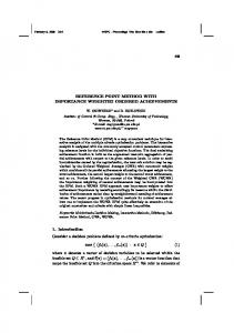
where λi+ > λi− are positive scaling factors corresponding to underachievements and overachievements, respectively, for the ith outcome. It is usually assumed that λi+ is much larger than λi− . Figure 1 depicts how differentiated scaling affects the isoline contours of the scalarizing achievement function.

(2)

where ε is an arbitrary small positive number and si : R →R, for i = 1, 2, . . . , m, are the partial achievement functions measuring actual achievement of the individual outcomes yi with respect to the corresponding reference levels. Let ai denote the partial achievement for the ith outcome (ai = si (yi )) and a = (a1 , a2 , . . . , am ) represent the achievement vector. The scalarizing achievement function (2) is, essentially, defined by the worst partial (individual) achievement but additionally regularized with the sum of all partial achievements. The regularization term is introduced only to guarantee the solution efficiency in the case when 18

the maximization of the main term (the worst partial achievement) results in a non-unique optimal solution. Due to combining two terms with arbitrarily small parameter ε , formula (2) is easily implementable and it provides a direct interpretation of the scalarizing achievement function as expressing utility. Various functions si provide a wide modeling environment for measuring partial achievements [5], [9]–[11]. The basic RPM model is based on a single vector of the reference levels, the aspiration vector ra . For the sake of computational simplicity, the piecewise linear functions si are usually employed. In the simplest models, they take a form of two segment piecewise linear functions:

Fig. 1. Isoline contours for the scalarizing achievement function (2) with partial achievements (3).

Real-life applications of the RPM methodology usually deal with more complex partial achievement functions defined with more than one reference point [5] which enriches the preference models and simplifies the interactive analysis. In particular, the models taking advantages of two reference vectors: vector of aspiration levels ra and vector of reservation levels rr [3] are used, thus allowing the DM to specify requirements by introducing acceptable and required values for several outcomes. The partial achieve-

Reference Point Method with Importance Weighted Partial Achievements

ment function si can be interpreted then as a measure of the DM’s satisfaction with the current value of outcome the ith criterion. It is a strictly increasing function of outcome yi with value ai = 1 if yi = ria , and ai = 0 for yi = rir . Thus the partial achievement functions map the outcomes values onto a normalized scale of the DM’s satisfaction. Various functions can be built meeting those requirements. We use the piece-wise linear partial achievement function introduced in an implementation of the ARBDS system for the multiple criteria transshipment problems with facility location [12]:  yi − r r   yi ≤ rir γ a ir ,   ri − ri     y − rr i i rir < yi < ria (4) si (yi ) = a − rr , r  i i     y − ra   α ai ir + 1, yi ≥ ria , ri − ri

where α and γ are arbitrarily defined parameters satisfying 0 < α < 1 < γ . Parameter α represents additional increase of the DM’s satisfaction over level 1 when a criterion generates outcomes better than the corresponding aspiration level. On the other hand, parameter γ > 1 represents dissatisfaction connected with outcomes worse than the reservation level. For outcomes between the reservation and the aspiration levels, the partial achievement function si can be interpreted as a membership function µi for a fuzzy target. However, such a membership function remains constant with value 1 for all outcomes greater than the corresponding aspiration level, and with value 0 for all outcomes below the reservation level (Fig. 2). Hence, the fuzzy membership function

is consistent with the fuzzy methodology in the case of not attainable aspiration levels and satisfiable all reservation levels while modeling a reasonable utility for any values of aspiration and reservation levels.

3. Ordered Weighted Averages Refinement of the RPM The crucial properties of the RPM are related to the maxmin aggregation of partial achievements while the regularization is only introduced to guarantee the aggregation monotonicity. Unfortunately, the distribution of achievements may make the max-min criterion partially passive when one specific achievement is relatively very small for all the solutions. Maximization of the worst achievement may then leave all other achievements unoptimized. Nevertheless, the selection is then made according to linear aggregation of the regularization term instead of the maxmin aggregation, thus destroying the preference model of the RPM. This can be illustrated with an example of a simple discrete problem of 7 alternative feasible solutions to be selected according to 6 criteria. Table 1 presents six partial achievements for all the solutions where the partial achievements have been defined according to the aspiration/reservation model (4) thus allocating 1 to outcomes reaching the corresponding aspiration level. All the solutions are efficient. Solution S1 to S5 oversteps the aspiration levels (achievement values 1.2) for four of the first five criteria while failing to reach one of them and the aspiration level for the sixth criterion as well (achievement values 0.3). Solution S6 meets the aspiration levels (achievement values 1.0) for the first five criteria while failing to reach only the aspiration level for the sixth criterion (achievement values 0.3). All the solutions generate the same worst achievement value 0.3 and the final selection of the RPM depends on the total achievement (regularization term). Actually, one of solutions S1 to S5 will be selected as better than S6. Table 1 Sample achievements with passive max-min criterion

Fig. 2. Partial achievement function (4).

is neither strictly monotonic nor concave thus not representing typical utility for a maximized outcome. The partial achievement function (4) can be viewed as an extension of the fuzzy membership function to a strictly monotonic and concave utility. One may also notice that the aggregation scheme used to build the scalarizing achievement function (2) from the partial ones may also be interpreted as some fuzzy aggregation operator [5]. In other words, maximization of the scalarizing achievement function (2)

Solutions

a1

a2

a3

a4

a5

a6

min

S1 S2 S3 S4 S5 S6 S7

0.3 1.2 1.2 1.2 1.2 1.0 0.3

1.2 0.3 1.2 1.2 1.2 1.0 0.3

1.2 1.2 0.3 1.2 1.2 1.0 0.3

1.2 1.2 1.2 0.3 1.2 1.0 1.0

1.2 1.2 1.2 1.2 0.3 1.0 0.6

0.3 0.3 0.3 0.3 0.3 0.3 1.0

0.3 0.3 0.3 0.3 0.3 0.3 0.3

∑ 5.4 5.4 5.4 5.4 5.4 5.3 3.5

In order to avoid inconsistencies caused by the regularization, the max-min solution may be regularized according to the ordered averaging rules [13]. This is mathematically formalized as follows. Within the space of achievement 19

Włodzimierz Ogryczak

vectors we introduce map Θ = (θ1 , θ2 , . . . , θm ) which orders the coordinates of achievements vectors in a nondecreasing order, i.e., Θ(a1 , a2 , . . . , am ) = (θ1 (a), θ2 (a), . . . , θm (a)) iff there exists a permutation τ such that θi (a) = aτ (i) for all i and θ1 (a) ≤ θ2 (a) ≤ . . . ≤ θm (a). The standard maxmin aggregation depends on maximization of θ1 (a) and it ignores values of θi (a) for i ≥ 2. In order to take into account all the achievement values, one needs to maximize the weighted combination of the ordered achievements thus representing the so-called ordered weighted averaging aggregation [13]. Note that the weights are then assigned to the specific positions within the ordered achievements rather than to the partial achievements themselves. With the OWA aggregation one gets the following RPM model: m

max

∑

(5)

wi θi (a) ,

i=1

criteria model. Actually, even complicated partial achievement functions of the form (4) are strictly increasing and concave, thus allowing for implementation of the entire RPM model (2) by an location problem (LP) expansion [12]. The OWA aggregation is obviously a piecewise linear function since it remains linear within every area of the fixed order of arguments. The ordered achievements used in the OWA aggregation are, in general, hard to implement due to the pointwise ordering. Its optimization can be implemented by expressing in terms of the cumulated ordered achievements θ¯k (a) = ∑ki=1 θi (a) expressing, respectively: the worst (smallest) achievement, the total of the two worst achievements, the total of the three worst achievements, etc. Indeed, m

∑

i=1

m

wi θi (a) = ∑ w′i θ¯i (a) , i=1

where w1 > w2 > . . . > wm > 0 are positive and strictly decreasing weights. Actually, they should be significantly decreasing to represent regularization of the max-min order. When differences among weights tend to infinity, the OWA aggregation approximates the leximin ranking of the ordered outcome vectors [14]. Note that the standard RPM model with the scalarizing achievement function (2) can be expressed as the following OWA model [15]: ! ε ε m max (1 + )θ1 (a) + ∑ θi (a) . m m i=2

where w′i = wi − wi+1 for i = 1, . . . , m − 1, and w′m = wm . This simplifies dramatically the optimization problem since quantities θ¯k (a) can be optimized without use of any integer variables [6]. First, let us notice that for any given vector a, the cumulated ordered value θ¯k (a) can be found as the optimal value of the following LP problem:

Hence, the standard RPM model exactly represents the OWA aggregation (5) with strictly decreasing weights in the case of m = 2 (w2 = ε /2 < w1 = 1 + ε /2). For m > 2 it abandons the differences in weighting of the largest achievement, the second largest one, etc., (w2 = . . . = wm = ε /m). The OWA RPM model 5 allows one to distinguish all the weights by introducing increasing series (e.g., geometric ones). One may notice in Table 2 that application of decreasing weights w = (0.5, 0.25, 0.15, 0.05, 0.03, 0.02) within the OWA RPM enable selection of solution S6 from Table 1.

The above problem is an LP for a given outcome vector a while it becomes nonlinear for a being a vector of variables. This difficulty can be overcome by taking advantage of the LP dual to (6). Introducing dual variable tk corresponding to the equation ∑m i=1 uik = k and variables dik corresponding to upper bounds on uik one gets the following LP dual of problem (6):

Table 2 Ordered achievements values Solutions S1 S2 S3 S4 S5 S6 S7 w

θ1 0.3 0.3 0.3 0.3 0.3 0.3 0.3 0.5

θ2 0.3 0.3 0.3 0.3 0.3 1.0 0.3 0.25

θ3 1.2 1.2 1.2 1.2 1.2 1.0 0.3 0.15

θ4 1.2 1.2 1.2 1.2 1.2 1.0 0.6 0.05

θ5 1.2 1.2 1.2 1.2 1.2 1.0 1.0 0.03

θ6 1.2 1.2 1.2 1.2 1.2 1.0 1.0 0.02

Aw 0.525 0.525 0.525 0.525 0.525 0.650 0.305

An important advantage of the RPM depends on its easy implementation as an expansion of the original multiple 20

m

θ¯k (a) = min { ∑ ai uik : uik

m

i=1

∑ uik = k, 0 ≤ uik ≤ 1

(6)

∀i } .

i=1

m

θ¯k (a) = max {ktk − ∑ dik : tk ,dik

ai ≥ tk − dik , dik ≥ 0

i=1

(7)

∀ i }.

Due the duality theory, for any given vector a the cumulated ordered coefficient θ¯k (a) can be found as the optimal value of the above LP problem. It follows from (7) that θ¯k (a) = max {ktk − ∑m i=1 (tk − ai )+ }, where (.)+ denotes the nonnegative part of a number and tk is an auxiliary (unbounded) variable. The latter, with the necessary adaptation to the minimized outcomes in location problems, is equivalent to the computational formulation of the k–centrum model introduced by [16]. Hence, formula (7) provides an alternative proof of that formulation. Taking advantages of the LP expression (7) for θ¯i the entire OWA aggregation of the partial achievement functions (5) can be expressed in terms of LP. Moreover, in the case of concave piecewise linear partial achievement functions (as typically used in the RPM approaches), the resulting for-

Reference Point Method with Importance Weighted Partial Achievements

mulation extends the original constraints and criteria with linear inequalities. In particular, for strictly increasing and concave partial achievement functions (4), it can be expressed in the form: m

max ∑ w′k zk s.t.

k=1 m

zk = ktk − ∑ dik

∀k

x ∈ Q, yi = fi (x)

∀i

ai ≥ tk − dik , dik ≥ 0

∀ i, k

ai ≤ γ (yi − rir )/(ria − rir ) ai ≤ (yi − rir )/(ria − rir ) ai ≤ α (yi − ria )/(ria − rir ) + 1

∀i

i=1

(8)

∀i ∀ i.

then those related to the second criterion. To take into account the importance weights in the WOWA aggregation (9) we introduce piecewise linear function ( for 0 ≤ ξ ≤ 0.5 0.9ξ /0.5 ∗ w (ξ ) = 0.9 + 0.1(ξ − 0.5)/0.5 for 0.5 < ξ ≤ 1.0 and calculate weights ωi according to formula (10) as w∗ increments corresponding to importance weights of the ordered outcomes, as illustrated in Fig. 3. In particular, one gets ω1 = w∗ (p1 ) = 0.95 and ω2 = 1 − w∗ (p1 ) = 0.05 for vector a′ while ω1 = w∗ (p2 ) = 0.45 and ω2 = 1 − w∗ (p2 ) = 0.55 for vector a′′ . Finally, Aw,p (a′ ) = 0.95 · 1 + 0.05 · 2 = 1.05 and Aw,p (a′′ ) = 0.45 · 1 + 0.55 · 2 = 1.55. Note that one may alternatively compute the WOWA values by using the importance weights to replicate corresponding achievements and calculate then OWA aggregations. In the case of our importance weights p we need to consider three copies of achievement a1 and one copy of achievement a2

4. Weighted OWA Enhancement Typical RPM model allows weighting of several achievements only by straightforward rescaling of the achievement values [8]. The OWA RPM model enables one to introduce importance weights to affect achievement importance by rescaling accordingly its measure within the distribution of achievements as defined in the so-called weighted OWA aggregation [7], [17]. Let w = (w1 , . . . , wm ) and p = (p1 , . . . , pm ) be weighting vectors of dimension m such that wi ≥ 0 and pi ≥ 0 for i = 1, 2, . . . , m as well as m ∑m i=1 pi = 1 (typically it is also assumed ∑i=1 wi = 1 but it is not necessary in our applications). The corresponding weighted OWA aggregation of outcomes a = (a1 , . . . , am ) is defined as follows [7]: m

Aw,p (a) = ∑ ωi θi (a) ,

(9)

i=1

where the weights ωi are defined as

ωi = w∗ ( ∑ pτ (k) ) − w∗ ( ∑ pτ (k) ) , k≤i

(10)

k