Geosci. Model Dev., 7, 1855–1872, 2014 www.geosci-model-dev.net/7/1855/2014/ doi:10.5194/gmd-7-1855-2014 © Author(s) 2014. CC Attribution 3.0 License.
Refinement of a model for evaluating the population exposure in an urban area J. Soares1 , A. Kousa2 , J. Kukkonen1 , L. Matilainen2 , L. Kangas1 , M. Kauhaniemi1 , K. Riikonen1 , J.-P. Jalkanen1 , T. Rasila1 , O. Hänninen3 , T. Koskentalo2 , M. Aarnio1 , C. Hendriks4 , and A. Karppinen1 1 Finnish
Meteorological Institute, Erik Palménin aukio 1, P.O. Box 503, 00101 Helsinki, Finland Region Environmental Services Authority P.O. Box 521, 00521 Helsinki, Finland 3 National Institute for Health and Welfare, P.O. Box 95, 70701 Kuopio, Finland 4 TNO, department of Climate, Air and Sustainability, Utrecht, The Netherlands 2 Helsinki
Correspondence to: J. Soares (
[email protected]) Received: 16 February 2014 – Published in Geosci. Model Dev. Discuss.: 10 April 2014 Revised: 15 July 2014 – Accepted: 25 July 2014 – Published: 2 September 2014
Abstract. A mathematical model is presented for the determination of human exposure to ambient air pollution in an urban area; the model is a refined version of a previously developed mathematical model EXPAND (EXposure model for Particulate matter And Nitrogen oxiDes). The model combines predicted concentrations, information on people’s activities and location of the population to evaluate the spatial and temporal variation of average exposure of the urban population to ambient air pollution in different microenvironments. The revisions of the modelling system containing the EXPAND model include improvements of the associated urban emission and dispersion modelling system, an improved treatment of the time use of population, and better treatment for the infiltration coefficients from outdoor to indoor air. The revised model version can also be used for estimating intake fractions for various pollutants, source categories and population subgroups. We present numerical results on annual spatial concentration, time activity and population exposures to PM2.5 in the Helsinki Metropolitan Area and Helsinki for 2008 and 2009, respectively. Approximately 60 % of the total exposure occurred at home, 17 % at work, 4 % in traffic and 19 % in other microenvironments in the Helsinki Metropolitan Area. The population exposure originating from the long-range transported background concentrations was responsible for a major fraction, 86 %, of the total exposure in Helsinki. The largest local contributors were vehicular emissions (12 %) and shipping (2 %).
1
Introduction
Exposure models vary from simple relations of the health aspects with the outdoor air concentrations up to comprehensive deterministic exposure models (e.g. Kousa et al., 2002; Ashmore and Dimitripoulou, 2009). Most of the epidemiological studies have been conducted based on relations between pollution concentrations measured at fixed ambient air quality monitoring sites, or modelled values using land-use regression models, and community-level health indicators, such as mortality (Pope and Dockery, 2006). Since the urban population spends typically 80–95 % of their time indoors (Hänninen et al., 2005; Schweizer et al., 2007), the exposure to particles is dominated by exposure in indoor environments. The most simplistic approaches ignore the differences between indoor and outdoor air. Indoor air quality is determined by infiltration, ventilation and indoor pollution sources. Infiltration of outdoor particles indoors can be significant even in tight buildings that use mechanical ventilation systems and efficient air intake filters. Infiltration can also occur due to the operation of windows and doors, and cracks in the building envelope and window and door frames (Hänninen et al., 2005). Population exposure can therefore be significantly different, depending on the structure and ventilation of buildings. If one only takes into consideration concentration levels at measurement sites, fine-scale spatial variability is disregarded. However, the concentrations of pollutants in urban areas may vary by an order of magnitude on a scale of tens of metres. This is particularly important for traffic-originated
Published by Copernicus Publications on behalf of the European Geosciences Union.
1856
J. Soares et al.: Refinement of a model for evaluating the population exposure
pollution. Moreover, most of the simplistic models ignore the activity patterns of individuals, i.e. people’s day-to-day movements from one location to another, which is known to cause significant variations in exposure (Beckx et al., 2009). The assessment of exposure with a deterministic approach usually requires application of integrated model chains starting from estimation of emissions to atmospheric dispersion and transformation of air pollutants. This can be complemented with time–microenvironment–activity models, an essential part of exposure assessment, and indoor to outdoor (i / o) concentration ratios. Microenvironment is defined by a location in which human exposure takes place, containing a relatively uniform concentration, such as, e.g. home or workplace. The average personal or population exposure is then estimated as a linear combination of concentrations in different microenvironments, weighted by the time spent in each of them. Probabilistic models of population exposure distributions such as EXPOLIS (Hänninen et al., 2003, 2005) and INDAIR (Dimitroulopoulou et al., 2006) provide the frequency distribution of exposure within a population, rather than mean or individual exposures. The population exposure can also be obtained by combining time activity, dispersion modelling, and Geographical Information Systems techniques; this approach has been adopted in the models developed by Jensen (1999), Kousa et al. (2002), Gulliver and Briggs (2005), Beckx et al. (2009) and Borrego et al. (2009). These models can evaluate the individual or population exposure in different microenvironments during the day. In particular, the deterministic modelling system EXPAND (EXposure model for Particulate matter And Nitrogen oxiDes; Kousa et al., 2002) can be applied to continuous time segments ranging from 1 h to several years, and for various urban spatial domains, as the time activity and emission data are temporally and spatially resolved. The city-scale resolution allows taking into consideration small-scale (street and neighbourhood scales) spatial variability. The EXPAND model can also consider exposure pathways, by evaluating population intake fractions (Loh et al., 2009). The EXPAND model was developed for the determination of human exposure to ambient air pollution in an urban area. The aims of this paper are to describe a substantially improved version of this model and to present selected illustrative numerical results. Numerical results were computed for human exposure to fine particulate matter (PM2.5 ) in the Helsinki Metropolitan Area for 2008 and in Helsinki for 2009. The Helsinki Metropolitan Area is located by the Baltic Sea and is comprised of four cities: Helsinki, Espoo, Vantaa and Kauniainen; the total population is slightly over 1.0 million. The population of Helsinki is over 600 000. We have evaluated the exposure of the population in terms of both various microenvironments and the main source categories. This study also presents for the first time quantitative evaluations of the influence of shipping emissions on concentrations and population exposure in Helsinki. Geosci. Model Dev., 7, 1855–1872, 2014
2 2.1
Methodology Modelling of vehicular traffic flows
We have modelled the traffic flows in the street network of the Helsinki Metropolitan Area using the EMME/2 interactive transportation planning package (INRO, 1994). The model generates a treatment for the traffic demand on the basis of given scenarios, and allocates the activity over the links (i.e. segments of road or street) of this network, according to a predetermined set of rules and individual link characteristics (Elolähde, 2006). The traffic demand generated by the model is governed by the assumed socio-economic urban structure and location of the main activities, such as residential areas and workplaces, as well as the usage rate of public transport. Both the urban bus routes and the incoming and outgoing coach traffic are included in the model. According to the link characteristics and the number of vehicles, the software is used to compute the average speed of vehicular traffic for each link on a given hour of the day. Furthermore, both weekly and seasonal variations of the traffic density are taken into account. The profiles of vehicle speed and vehicle numbers are then computed for each link for each hour of the day (separately for weekdays, Saturdays and Sundays), and further aggregated over the year. In this study, approximately 4300 road and street links were included in the computations. The model also allows for the activities at all the major ports in Helsinki – which increase heavy duty vehicle traffic, in particular. In this study, the traffic flow modelling was based on the traffic data for 2008 and 2009, for the corresponding dispersion computations for 2008 and 2009, respectively. It was pertinent to use up-to-date traffic data, due to recent substantial changes of traffic flows, caused especially by a recently constructed major cargo harbour in the easternmost part of Helsinki at Vuosaari. This new harbour is located further away from the Helsinki city centre, and it has been active since November 2008. The container terminals of the harbours at Sörnäinen and at the western harbour (which are located in central Helsinki) were transferred to the harbour at Vuosaari. 2.2
Modelling of emissions
The emissions of PM2.5 were evaluated in the Helsinki Metropolitan Area for 2008, and in a more limited domain, the city of Helsinki for 2009. We have included the emissions originated from urban vehicular traffic for both years, and the emissions from shipping and major stationary sources for 2009. This approach has allowed us to study both the general characteristics of population exposure in the whole of the metropolitan area, and in more detail the influence of two potentially significant local source categories in the capital city.
www.geosci-model-dev.net/7/1855/2014/
J. Soares et al.: Refinement of a model for evaluating the population exposure 2.2.1
Exhaust and suspension emissions originated from vehicular traffic
The emissions of PM2.5 were computed for each link using average speed-dependent functions, determined separately for each vehicle category (Laurikko et al., 2003). The emission factors were based on European emission factors, and these take into account the age distribution of the Finnish vehicle fleet (Kauhaniemi et al., 2011; Laurikko et al., 2003). A total of 14 vehicle categories were included, divided into petrol cars with or without a catalytic converter, dieselfuelled vehicles, as well as buses and other heavy duty vehicles. The division of the vehicles within the passenger car category was based on the registration statistics. We evaluated the vehicular-traffic emissions by scaling a previously compiled detailed inventory for the year 2005, to correspond to the years 2008 and 2009. The national vehicular exhaust emission values are available for 2005, 2008 and 2009 from a calculation system for traffic exhaust emissions and energy consumption, LIPASTO (Mäkelä, 2002). The scaling was performed for each road link, mainly using the ratio of the total vehicular exhaust emissions of PM2.5 in Helsinki Metropolitan Area in 2005 to that in 2008 and 2009, respectively. This means that the vehicular exhaust emissions were assumed to vary with a constant percentage from 2005 to 2008 or 2009. In addition, this scaling allows for major changes in traffic flows, such as those caused by the transferred cargo harbours. In the Nordic countries, the cold start and cold driving emissions of PM2.5 can be substantial, especially in winter. These emissions were taken into account, using coefficients based on laboratory emission measurements (Laurikko, 1998). The coefficients were estimated separately for weekdays and weekend, and take into consideration the temperature of ambient air and the fraction of vehicles using a pre-heating of engine (Kauhaniemi et al., 2008). We also applied a model for the road suspension emissions for PM2.5 , FORE, described by Kauhaniemi et al. (2011). This model is based on the model presented by Omstedt et al. (2005). The emission factor for suspension of road dust (in units µg veh−1 m−1 ) is a product of the so-called reference emission factors, the reduction factor of the moisture content of the street, and a weighted sum of the contribution of particles from the wear of pavement and from the traction sand. The FORE model can be used as an assessment tool for urban PM2.5 contributions in various European regions, provided that the model input values are available for local traffic flow, meteorological data and region-specific coefficients. The region-specific coefficients can be determined with fairly simple measurements, as described by Omstedt et al. (2005). However, the emissions from brake, tyre and clutch wear are not included in the model, due to their small contribution compared to suspension and road wear emissions in the Nordic countries. The baseline values for the suspension www.geosci-model-dev.net/7/1855/2014/
1857
emission model were set by the reference emission factors that depend on the period (which may include street sanding or not), the mass fraction of particles (fine and coarse), and the traffic environment (urban or highway). 2.2.2
Emissions originated from shipping
Emissions from ship traffic in the harbours of Helsinki and in the surrounding sea areas were modelled using the Ship Traffic Emissions Assessment Model (STEAM) presented by Jalkanen et al. (2009, 2012). The method is based on using the messages provided by the Automatic Identification System (AIS), which enable the positioning of ship emissions with a high spatial resolution (typically a few tens of metres). The model also takes into account the detailed technical data of each individual vessel. The AIS messages were received from the Finnish AIS network. The geographical domain of ship emission modelling was selected so that all the major harbours in Helsinki were included. We modelled the emissions (i) from ships cruising in the selected domain in the vicinity of Helsinki; (ii) from ships manoeuvring in harbours; and (iii) from the use of diesel generators at ships while at berth. Emissions from other sources in harbours, such as various harbour machinery, were not included. The computational domain of the shipping emissions comprises a rectangular area, the extent of which is 21.5 km in the east to west direction, and 25.5 km in the north to south direction. The cell size of the computational grid is 0.001◦ . This domain is slightly larger than the computational domain for evaluating exposures, as we considered it appropriate to include also the shipping emissions originated from the sea areas in the vicinity of Helsinki. 2.2.3
Emissions originated from stationary sources
The emissions from major stationary sources in the Helsinki Metropolitan Area mainly originated from energy production and other industrial sources. We have allowed for the most widely used methods for heating of residential buildings and domestic water, and for household appliances, namely electricity (33 %) and district heating (29 %) (Statistics Finland, 2012). The third most important source of energy for households is small-scale combustion, which mainly consists of the burning of wood (23 %). However, small-scale combustion was not included in this study, as the spatial distribution of the emission data was not known with sufficient accuracy. 2.3
Dispersion modelling
The urban atmospheric dispersion modelling system utilized in this study combines the road network dispersion model CAR-FMI (Contaminants in the Air from a Road) for vehicular traffic and shipping, and the UDM-FMI model (Urban Dispersion Model) for stationary sources. These models have Geosci. Model Dev., 7, 1855–1872, 2014
1858
J. Soares et al.: Refinement of a model for evaluating the population exposure
been addressed in detail by, e.g. Karppinen et al. (2000a) and Kukkonen et al. (2001). Both of these models are multiplesource Gaussian urban dispersion models. The dispersion parameters are modelled as a function of Monin–Obukhov length, friction velocity and boundary layer height, which are computed with meteorological preprocessing model MPP-FMI (Karppinen, 2001). This model has been used with input data from the three nearest synoptic weather stations and the nearest sounding station, to evaluate an hourly meteorological time series for the dispersion modelling computations. In the urban-scale computations, PM2.5 was treated as a tracer contaminant, i.e. no chemical reactions or aerosol processes were included in the calculations. The computations included approximately 5000 line sources for vehicular traffic and shipping for both years, and in addition, 40 stationary sources (power plants and industrial facilities) for 2009. All shipping emissions were treated as line sources with an injection height of 30 m above the sea level. The value of 30 m is a weighted average value of the injection heights of all ships considered (including also their estimated average plume rise); as relative weighting coefficients we used the magnitudes of emissions provided by the STEAM model. The STEAM model includes a detailed database that contains technical properties of all major ships that travel in the Baltic Sea. For 2008, the regional and long-range transported (LRT) background concentrations were based on the concentrations computed with the LOTOS-EUROS model (Schaap et al., 2008). We selected as the LRT background values the predicted hourly PM2.5 concentrations at a model grid square (approximately of the size of 7 × 7 km2 ) that includes the regional background station Luukki. This site has previously been found to represent well the LRT background concentrations for the Helsinki Metropolitan Area; the influence of local sources on the PM2.5 concentrations at this station has been estimated to be on average less than 10 %. The reason for using the predictions of the LOTOS-EUROS model was the harmonization of regional background computations in the EU-funded TRANSPHORM project (www.transphorm. eu). However, for 2009, we used as the LRT background concentrations the measured values at the measurement site in Luukki. The computations of the LOTOS-EUROS model on a European scale included the formation of secondary inorganic aerosol, including sulfates, nitrates and ammonia, but these did not include the formation of secondary organic aerosol. The contributions from sea salt, wild-land fires and elemental carbon have also been included. The secondary PM2.5 has therefore been modelled with a reasonable accuracy in the regional background concentration values; however, there is an underprediction, caused presumably mainly by the missing secondary organic aerosol fraction. The local contribution of sea salt aerosol in PM2.5 is on average smaller than 0.2 µg m−3 in Helsinki; the low value is Geosci. Model Dev., 7, 1855–1872, 2014
mainly due to the low salinity of the Baltic Sea (Sofiev et al., 2011). The wind-blown dust concentrations are also low on an annual average level, emitted by distant sources (Franzen et al., 1994). Hence, the urban-scale computation included only the LRT contribution of these natural aerosols. The concentrations were computed in an adjustable grid. The receptor grid intervals ranged from approximately 20 m in the vicinity of the major roads to 500 m on the outskirts of the area. The number of receptor points was more than 18 000 and more than 6000 for the computations of vehicular traffic and shipping, and for the stationary sources, respectively. The CAR-FMI model has previously been evaluated against the measured data of urban measurement networks in Helsinki Metropolitan Area and in London both for gaseous pollutants (e.g. Karppinen et al., 2000b; Kousa et al., 2001; Hellén et al., 2005) and for PM2.5 (Kauhaniemi et al., 2008; Sokhi et al., 2008; Singh et al., 2014). The performance of the CAR-FMI model has also been evaluated against the results of a field measurement campaign and other roadside dispersion models (Kukkonen et al., 2001; Öttl et al., 2001; Levitin et al., 2005). The UDM-FMI has been evaluated against the measured data of urban measurement networks in Helsinki Metropolitan Area (Karppinen et al., 2000b; Kousa et al., 2001) and the tracer experiments of Kincaid, Copenhagen and Lilleström. The main limitation of Gaussian dispersion models is that they do not allow for the detailed structure of buildings and obstacles. 2.4
Modelling of human activities
We obtained the information on the location of the population from the data set that has been collected annually by the municipalities of the Helsinki Metropolitan Area. The human activity data within the EXPAND model are based on this data set. The data set contains information on the dwelling houses, enterprises and agencies located in the area in 2009. The data set provides geographic information on the total number and age distribution of people living in a particular building, and the total number of people working at a particular workplace. The data also include information on the number and location of customers in shops and restaurants, and individuals in other recreational activities. The location of people in traffic was evaluated using the computed traffic flow information. This information is available separately for buses, cars, trains, trams, metro, pedestrians and cyclists for each street and rail section on an hourly basis. Neither this information nor the above-mentioned information from the municipalities identifies individual persons. Time activity of people in harbours was based on the numbers of travellers in each ship line and the timetables of ships arriving to and departing from Helsinki. The time–microenvironment activity data for both years considered (2008 and 2009) is based on the time use survey by Statistics Finland. The time activity data were collected www.geosci-model-dev.net/7/1855/2014/
J. Soares et al.: Refinement of a model for evaluating the population exposure from 532 randomly selected over-10-year-old inhabitants in the Helsinki Metropolitan Area for the years 2009 and 2010 (OSF, 2013). There was no detailed information on the time activities of children that are younger than or equal to 10 years old; it was therefore assumed in the activity modelling that such children stay at home all the time. This assumption will probably result in only moderate inaccuracies, as most of the childcare facilities and schools are located within a radius of three kilometres of a child’s home. Population time activity data were divided into four microenvironments: home, workplace, traffic and other activities. The category “other activities” includes customers in shops, restaurants and other locations; however, it does not include the personnel working at such places (they are included in the category “workplace”). The time activity data are updated by the municipalities once in every 10 years. The data that we have used in this study (corresponding to the year 2009) are therefore better representative for the last few years than the data used in the previous EXPAND model version (Kousa et al., 2002). The previously applied time– microenvironment activity data were provided for Helsinki in the EXPOLIS study. The EXPOLIS activity data included only adult urban populations, from 25 to 55 years of age, whereas the new activity data include all population age groups. 2.5
The infiltration of outdoor air indoors
Indoor air quality is determined by the efficiency of infiltration of outdoor air indoors, ventilation and indoor air pollution sources. An infiltration factor (Finf ) for pollutant species a is defined as Finf =
Cai , Ca
(1)
where Cai is the indoor air concentration of species a originating from ambient air, and Ca is the outdoor air concentration of species a. By definition 0 ≤ Finf ≤ 1. The infiltration rates of ambient air particles in the previous version of the EXPAND model were estimated using data based on the EXPOLIS study. This was a population representative study on working age people, conducted in 1996– 1997. It included measurements of indoor and outdoor PM2.5 concentrations, and X-ray fluorescence analysis of elemental markers (Hänninen et al., 2004; Jantunen et al., 1998; Rotko et al., 2000). Elemental sulfur was used as a marker of the outdoor originating particles in 84 residences. The i / o ratios of sulfur in particles were also corrected to allow for the particle size distributions (Hänninen et al., 2004). The infiltration factors at workplaces of the same subjects were also analysed. The workplaces are distributed following a random population sample, but differences between different types of workplaces could not be evaluated, due to the limited number of subjects. Data on infiltration factors in public buildings are scarce; it has therefore been assumed www.geosci-model-dev.net/7/1855/2014/
1859
that the values determined in the EXPOLIS project correspond to all workplaces. In this study, the previous EXPOLIS infiltration estimates were updated, using also aerosol measurements in the ULTRA-2 study. These aerosol samples were collected in Helsinki in 1999, including a sample of homes of 47 cardiovascular patients, with 4–5 repeated measurements (Lanki et al., 2008). The set of homes is smaller in this sample, but the methods were updated to include a treatment of particle-sizedependent behaviour. The comparison of the results obtained using sulfur-based and aerosol methods revealed significant differences in the aerosol parameters – in particular, regarding the deposition rate and the estimation of the air exchange rates. Nevertheless, the PM2.5 infiltration factor distributions of residences were almost identical and were not affected by the improved methods. In this study, we have evaluated only the impact of outdoor air pollution on the population exposure. We have considered neither the influence of indoor sources of PM2.5 nor the impact of particulate matter transformation and deposition in the indoor environments on the population exposure. In order to account for the indoor concentrations, the EXPAND model could be used to consider the ratio between indoor and outdoor concentrations. However, the detailed value of this ratio depends on numerous factors, in particular the influence of indoor sources. The infiltration factors in the present study are based on the results that are summarized in Table 1. These PM2.5 infiltration rates were estimated based on residential and workplace measurements using two relatively large population-based data sets (EXPOLIS and ULTRA-2). We therefore evaluate that the residential infiltration rates have been fairly reliably estimated for the 1996–1999 building stock. The corresponding values for workplaces, representing partly public buildings and partly private occupational businesses, are available only from the EXPOLIS study. The infiltration estimates for non-residential buildings therefore contain more substantial uncertainties. For simplicity, a weighted average of the presented results, i.e. the value of 0.57, was assumed to represent both the home and work environments. As the information in the case of traffic and other microenvironments was very scarce, it was assumed that the infiltration factor would be equal to one for those microenvironments. The Finnish building code (EP, 2002) was updated in 2002 and 2010, setting new requirements for improved energy efficiency and improved filtration in ventilation. The infiltration rates will therefore be lower in buildings that have been built after the two above-mentioned studies. Hänninen et al. (2005) estimated that there was a 20 % reduction of infiltration factors in the building stock that was built in the 1990s, in comparison with older buildings. The same longterm trend has continued in the 2000s. Considering all buildings, the impact on infiltration factors of improved energy efficiency and filtration in ventilation is much smaller, due to Geosci. Model Dev., 7, 1855–1872, 2014
1860
J. Soares et al.: Refinement of a model for evaluating the population exposure
Table 1. Compilation of available results on the PM2.5 infiltration factors in the building stocks in the Helsinki Metropolitan Area, based on the results from the EXPOLIS and ULTRA-2 studies. In the case of the EXPOLIS study, the main references are listed. For the ULTRA-2 study, the methods are mentioned; these infiltration factors have not been previously published. SD = standard deviation.
Acronym of study EXPOLIS EXPOLIS ULTRA-2 ULTRA-2
Year
Type of buildings
Number of buildings
Infiltration factor (mean ± SD)
References method
1996–1997 1996–1997 1999 1999
Residences Workplaces Residences Residences
84 94 47 (180)∗ 47 (180)∗
0.59 ± 0.17 0.47 ± 0.24 0.58 ± 0.15 0.55 ± 0.13
Hänninen et al. (2004, 2011) Hänninen et al. (2005) Sulfur-based method (Hänninen et al., 2013) Aerosol-based method (Hänninen et al., 2013)
∗ Number of daily measurements in parentheses.
the slow renewal rate of the building stock, estimated to be of the order of 1–2 % annually. 2.6 Modelling of exposure Exposure to air pollutants can be represented as the sum of the products of time spent by a person in different locations and the averaged air pollutant concentrations prevailing in those locations. These locations are commonly categorized into microenvironments, which are assumed to have homogeneous pollutant concentrations. Exposure can therefore be written as Ei =
m X j =1
Tij Cij Ei =
m X
Tij Cij ,
(2)
j =1
where Ei is the total exposure of person i in various microenvironments [µg m−3 s], m is the number of different microenvironments, Tij is the time spent in microenvironment j by person i [s] and Cij is the air pollutant concentration that person i experiences in microenvironment j [µg m−3 ]. Equation (2) can also be interpreted as a weighted sum of concentrations, in which the weights are equal to the time spent in each microenvironment. The main objective of this study was to evaluate the average exposure of the population with reasonable accuracy, instead of the personal exposures of specific individuals. The exposure modelling in the case of homes is done by combining residential coordinates with the information on the number of inhabitants at each building and the time spent at home during each day. Correspondingly, for the workplace coordinates, the number of the personnel and the time spent at the workplace are combined. The population activities at other locations (such as shops, restaurants, cafes, pubs, cinemas, libraries and theatres) are evaluated using statistical information of leisure time (CHUF, 2009). The number of persons in traffic is evaluated based on the predicted traffic flows. In the case of buses, trains, metro, trams and pedestrians and cyclists, the number of persons and the time they spend in each street or rail section is estimated using the traffic-planning model EMME/2. Geosci. Model Dev., 7, 1855–1872, 2014
In the case of private cars, the EMME/2 model predicts the number of cars; we assumed that the number of passengers in each car is equal to the average value in the area, i.e. 1.31 (Hellman, 2012). The concentrations are interpolated on to a rectangular grid in the model. The data regarding population activities (number of persons × hour) is also converted to the same grid. For this study, the grid size was selected as 50 × 50 m2 . The GIS system MapInfo is subsequently utilized in the postprocessing and visualization of this information. The model has also been extended to be able to use various internationally used coordination systems; details are reported in Appendix A. 2.7
Modelling of intake fractions
The EXPAND model was refined to calculate not only exposures, but also intake fractions (iF) for the available substances. The iF is defined as intake by humans via relevant exposure pathways, divided by the emissions of the pollutant. For instance, an intake fraction of one in a million (10−6 ) means that for every tonne of a pollutant emitted, 1 g is inhaled by the exposed population. The iF concept provides a measure of the portion of a source’s emissions that is, e.g. inhaled by an exposed population over a defined period of time. The iF concept can be useful in both screening-level orderof-magnitude estimates and more detailed policy modelling of non-reactive compounds (Bennett et al., 2002). The model allows for the estimation of the spatial and temporal distribution of iFs, by combining and processing different input values: time–microenvironment activity data, the spatial location of the population, microenvironmental population breathing rates and pollutant concentration distributions (Loh et al., 2009). The emissions can be considered for one source only, or for a selected source category. The iF can be calculated using exposure estimates for the microenvironments of interest and the average breathing rate of a population, while in each microenvironment.
www.geosci-model-dev.net/7/1855/2014/
J. Soares et al.: Refinement of a model for evaluating the population exposure 3
1861
Results and discussion
We address results computed for two years, 2008 and 2009. The computations in 2008 address the Helsinki Metropolitan Area, whereas the computations in 2009 focus on the city of Helsinki. Both computations include the LRT pollution, and the vehicular emissions. However, the computations for 2009 additionally include the emissions from major stationary sources and the emissions from shipping in the vicinity and in the harbours of Helsinki. The computations for 2008 can therefore be used for examining the population exposure within a wider area (the whole of the Helsinki Metropolitan Area), whereas those for 2009 are useful for investigating, in particular, the influence of major stationary sources and shipping on the population exposure within the more limited area of the Finnish capital. 3.1
Predicted emissions of PM2.5
The total emissions of PM2.5 originated from vehicular traffic were 322 tonnes for the Helsinki Metropolitan Area in 2008, and 202 tonnes for Helsinki in 2009. The vehicular emissions include exhaust emissions (these include also cold start and driving) and road suspension emissions. The emissions of PM2.5 originated from ships were estimated to be 204 tonnes in Helsinki in 2009. The PM emissions originated from major stationary sources were 225 tonnes in Helsinki in 2009, according to Lappi et al. (2008). In summary, the total annual emissions from vehicular sources and from shipping were approximately the same in Helsinki in 2009, and the emissions from major stationary sources were slightly higher than those from vehicular or shipping sources. The emissions of PM2.5 originated from shipping in 2009 are presented in Fig. 1b. There are three main harbours in central Helsinki, listed from north to south: the Kulosaari harbour, the southern harbour and the western harbour. The emissions per unit area are largest within these three harbour areas. One reason for the relatively high shipping emissions in harbours is that auxiliary diesel engines are used for power generation while at berth; these engines have relatively high emissions per power output, compared with the main engines (Jalkanen et al., 2012). The second largest emissions occur along the main shipping routes from Helsinki to Tallinn (the southward ones) and to other major cities. The small-scale combustion emissions were not included in the dispersion computations, due to insufficient information regarding the spatial distribution and magnitudes of these emissions. The contribution of small-scale combustion to the total PM2.5 emissions in Helsinki Metropolitan Area has been estimated to be 15 %; this fraction is slightly lower than the corresponding one for stationary sources (21 %) (Niemi et al., 2009; Gröndahl et al., 2013). In the present study, allowing also for the emissions of small-scale combustion as reported in the above-mentioned studies, the contributions of the different emission source categories for PM2.5 in www.geosci-model-dev.net/7/1855/2014/
Figure 1. (a) Location of the harbours and the measurement sites in their vicinity in 2009. The notation for harbours: Katajanokka harbour (KH), southern harbour (SH), western harbour (WH); and for the measurement sites: Eteläranta (EM), Katajanokka (KH), western harbour (WM). The urban background measurement site at Kallio is also marked in the figure. (b) The predicted emissions of PM2.5 originated from shipping (g cell−1 ) in Helsinki in 2009; the size of each grid cell is 0.001◦ .
Helsinki in 2009 are 36 % for vehicular traffic, 23 % for major stationary sources, 23 % for shipping and 18 % for smallscale combustion. 3.2
Predicted concentrations of PM2.5
The predicted concentrations for vehicular emissions and LRT in 2008 are presented in Fig. 2. The centre of Helsinki is on a peninsula that is located approximately in the middle of the southern part of Fig. 2. The LRT is responsible for a substantial fraction of the total PM2.5 concentrations. The concentrations are highest in the vicinity of the main roads and streets, and in the centre of Helsinki. Figure 2 shows also the distinct influence of the ring roads number 1 (situated at a distance of about 8 km from the city centre) and number 3 Geosci. Model Dev., 7, 1855–1872, 2014
1862
J. Soares et al.: Refinement of a model for evaluating the population exposure
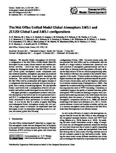
Figure 3. Predicted daily averaged against observed PM2.5 concentrations (µg m−3 ) at the stations of (a) Kallio (urban, background) and (b) Mannerheimintie (urban, traffic) in 2008.
Figure 2. Predicted annual average concentrations of PM2.5 (µg m−3 ) in the Helsinki Metropolitan Area in 2008. The grid size is 50 m × 50 m and the size of the depicted area is 20 km × 16 km.
(situated about 15 km from the city centre), the major roads leading to the Helsinki city centre, and the junctions of major roads and streets. The overall characteristics of the spatial distribution of the predicted concentrations in 2009 were very similar to those in 2008, and are therefore not presented here. Averaging the results, for 2008, over all receptor grid locations, shows that LRT, vehicular traffic and shipping contribute 86, 11 and 3 % to the PM2.5 concentrations, respectively. Although the average contribution of shipping to the total PM2.5 concentrations within the whole of the modelled domain was modest, this contribution can be higher than 20 % in the vicinity of the harbours (within a distance of approximately one kilometre). The computations for 2008 have been evaluated against the measurement data from the air quality monitoring network at the Helsinki Metropolitan Area; selected example results are presented in Fig. 3. In general, the agreement of the measured and predicted values was good or fairly good. For instance, the index of agreement that corresponds to the comparison of predicted and measured hourly time series of the PM2.5 concentrations varied from 0.72 to 0.73 at the available three stations, whereas the fractional bias varied from −0.16 to −0.22. It is appropriate to evaluate whether the above-mentioned values on the contribution of shipping and harbours on the PM2.5 concentrations are correct. We therefore compared the predicted annual average concentration values with the available measurements of the Helsinki Region Environmental Services Authority in the vicinity of harbours from 2008 to 2010 (Table 2). For two stations, the year of measurement was not the same as the predicted year (2009); these comparisons are therefore only qualitative. The measured data Geosci. Model Dev., 7, 1855–1872, 2014
included from 95 to 97 % of the hourly values for all these stations. Regarding the values at the stations in the vicinity of the harbours, the agreement of the predicted and measured annual means ranged from 5 to 9 %. This adds some confidence that the predicted contributions from shipping are probably approximately correct. The annual averages of the measured and predicted urban background values also differed only slightly. However, for the computations in 2009 we have used the measured regional background concentration values, which constitute a substantial fraction of the predicted concentrations. 3.3
Predicted time activities
The time activity of the population was divided into four categories: home, workplace, traffic and other activities. The diurnal variation of population activities in various microenvironments in the Helsinki Metropolitan Area is presented in Fig. 4. Children that are younger than or equal to 10 years have been excluded from the data of this figure; however, they are included in the subsequent exposure computations. In the data presented in Fig. 4, we have combined indoor and outdoor time activity in each microenvironment. On average people spend most of their time in the home environment. As expected, in the late afternoon and early evening, people spend a substantial fraction of their time in traffic and in other activities (these include shopping and various recreational activities). The results presented in Fig. 4 can be compared with the previously applied time activity data for the adult population presented by Kousa et al. (2002). As expected, the more comprehensive sample of the population presented in Fig. 4 (including population of all ages larger than 10 years) includes a substantially larger fraction of home activities, and a smaller fraction of work activities. The spatial and temporal distributions of the time activity were modelled separately for each microenvironment. The annually averaged results are presented in Fig. 5a–e. www.geosci-model-dev.net/7/1855/2014/
J. Soares et al.: Refinement of a model for evaluating the population exposure
1863
Table 2. Comparison between measured and predicted annual average PM2.5 concentrations (µg m−3 ) at the measurement sites in the vicinity of harbours, and at an urban background site in Helsinki. All modelled values are for 2009. SD = standard deviation based on the hourly values.
Name of the measurement site
Classification of the measurement site
Annual mean ± SD, modelled
Year of measurements
Annual mean ± SD, measured
Eteläranta Katajanokka Western harbour Kallio
In the vicinity of a harbour In the vicinity of a harbour In the vicinity of a harbour Urban background
8.7 ± 3.3 8.0 ± 2.9 8.2 ± 3.2 8.2 ± 3.0
2010 2009 2008 2009
9.8 ± 9.9 7.7 ± 6.0 8.7 ± 8.7 8.4 ± 5.7
Table 3. Contribution in each microenvironment to total time activity and exposure.
Microenvironment Home Work Traffic Other activity
Figure 4. The diurnal variation of the activity of the population in the Helsinki Metropolitan Area in four microenvironments, based on the data for 2009 and 2010. Children that are younger than or equal to ten years old have not been included in the statistics of this figure.
As expected, the population density values are highest in the centre of Helsinki (Fig. 5a). There are also elevated levels of population density in the vicinity of the district centres of the other major cities in the area (Espoo and Vantaa), and in the vicinity of major roads and streets. The work-time activities are focused in some regions of central Helsinki, in the district centres, and in some industrial areas, whereas the home activities, and partly also the other activities, are much more evenly dispersed throughout the area. 3.4 Predicted exposures to PM2.5 3.4.1
Exposures in various microenvironments in 2008
The population exposures were computed based on the predicted PM2.5 concentrations and time activities. The predicted concentration and population data were interpolated on to a rectangular grid with a grid size of 50 m. The population exposures were computed for each hour of the year, at 18.7 × 10³ receptor grid squares, separately for the selected four microenvironments. Population exposure is a combination of both the concentration and activity (or population density) values. The fractions of exposure in various microenvironments compared with the total population exposure to PM2.5 are presented in Fig. 6a These values include all age groups (including also www.geosci-model-dev.net/7/1855/2014/
Contribution to total time activity (%)
Contribution to total exposure (%)
61 18 2 18
60 17 4 19
children younger than 10 years). The exposure at home is responsible for most of the exposure, 60 %, whereas the work and other activities exposures are responsible for most of the rest of the exposure, i.e. 19 and 17 %, respectively. We have compared the shares of time activity and exposure in each microenvironment in Table 3, according to the computations. The contributions to the total time activity and exposure are similar for home, work and other activity microenvironments; this indicates that there are no major relative differences in the average concentrations prevailing at those microenvironments. However, for traffic the contribution to exposure is substantially higher than the corresponding contribution to time activity. This is mainly caused by the relatively higher concentrations on the roads and streets and in their vicinity. We have presented the spatial distributions of the predicted annual average population exposures in the Helsinki Metropolitan Area in 2008 in Fig. 7a–e, for the total exposure and separately for all microenvironments. These distributions exhibit characteristics of both the corresponding spatial concentration distributions and time activities. There are elevated values in the Helsinki city centre, along major roads and streets, and in the vicinity of urban district centres. The high home and work exposures in the centre of Helsinki are caused both by the relatively high concentrations and the highest population and workplace densities in the area. The spatial distributions of the population exposures at home and work correlate poorly (see Fig. 7b–c). The reason is that while most of the work environments are located either in the centre of Helsinki and in district centres, or in Geosci. Model Dev., 7, 1855–1872, 2014
1864
J. Soares et al.: Refinement of a model for evaluating the population exposure
Figure 5. The predicted density of population (no. persons), evaluated as an average for 2009 and 2010, for (a) all microenvironments, (b) home, (c) work, (d) traffic and (e) other activities. The grid size is 50 m × 50 m.
major industrial, service and commercial regions, a substantial fraction of residences are also located in suburban areas. As expected, the exposure while in traffic is focused along the main network of roads and streets, and in their immediate vicinity. These exposures may be under-predicted for three main reasons. First, the traffic flow and emission modelling
Geosci. Model Dev., 7, 1855–1872, 2014
does not completely allow for all the effects of traffic congestion. The traffic flow modelling does take into account the slowing down of traffic in certain regions and streets, and the emission modelling takes into account the dependency of emissions on the travel speed. However, the emission modelling does not take into account the effects of idling, and the
www.geosci-model-dev.net/7/1855/2014/
J. Soares et al.: Refinement of a model for evaluating the population exposure
Figure 6. Contribution to the total population exposures to PM2.5 : (a) in each microenvironment in the Helsinki Metropolitan Area in 2008, and (b) originated from various source categories in Helsinki, in 2009.
deceleration and acceleration of vehicles. Traffic congestion occurs frequently in the centre of Helsinki, and also along the main roads and streets, especially during rush hours. Second, the dispersion modelling and the spatial averaging does not allow for the very fine-scale (< 50 m) highest peak concentrations above the roads and streets. The dispersion modelling also does not include any treatment for dispersion in street canyons, which tends to result in an under-prediction of concentrations. Third, by assuming no indoor sources (the infiltration factor for vehicles is equal to one) the indoor concentrations are neglected. We have allowed for only the influence of outdoor air pollution on the population exposure. We have not addressed the indoor sources and sinks of pollution; however, indoor sources such as, e.g. tobacco smoking, cooking, heating and cleaning can cause additional short-term concentration maxima. We have also assumed that the infiltration factor is temporally constant. The temporal variation of indoor concentrations would be expected to be smoother than our assessments, due to the delay associated with the infiltration of outdoor air pollution to indoors. Such a delay would mainly affect shorter term exposure assessments; we consider only annual average exposures in the present study. 3.4.2
Exposures originated from various source categories in 2009
The population exposures from various source categories were also computed for each hour of the year. The contribution of each source category to the total population exposure to PM2.5 concentrations in Helsinki are presented in Fig. 6b. The population exposure originated from the LRT background concentrations is responsible for a major fraction, 86 %, of the total exposure. The next largest contributors are vehicular emissions (12 %) and shipping (2 %). The exposure originated from major stationary sources is negligible, caused by the dispersion of pollutants to wide regions due to high stacks for most of these installations. However, the above-mentioned percentage values include some uncertainties, due to excluding the small-scale combustion from www.geosci-model-dev.net/7/1855/2014/
1865
these computations. The contribution of small-scale combustion on the population exposure will be higher than its contribution to the total emissions, due to the low injection heights. We have presented in Fig. 8a–c the spatial distributions of annually averaged predicted population exposures to PM2.5 in Helsinki in 2009, originated from various source categories. The population exposure caused by shipping is focused in central Helsinki, near the main harbours and within some densely inhabited parts of the city. As expected, the population exposure is relatively substantially lower within the main park areas (e.g. Central Park, and the parks of Kaisaniemi and Kaivopuisto) and a cemetery (Hietaniemi). In the harbours and their vicinity (approx. 1 km from the harbour), the contribution of shipping to total exposure can reach up to 20 %.
4
Conclusions
We have presented a refined version of a mathematical model for the determination of human exposure to ambient air pollution. A review of the main characteristics of the previous and current versions of the EXPAND model are presented in Table 4. The revisions of the modelling system include the following: (i) the treatment of the time use of population has been extended to include all the age groups and a wide range of activities, including detailed treatments of the various traffic modes, and a wide range of recreational activities; (ii) the infiltration coefficients from outdoor to indoor air have been updated based on new information from the ULTRA-2 study; (iii) the revised model version can also be used for evaluating intake fractions, and the model can be applied using several internationally applied coordinate systems. The model can be used for evaluating specific population exposures, e.g. in terms of population age groups, microenvironments, source categories or individual sources. Numerical results are presented on the spatial concentrations, the time activity and the population exposures to PM2.5 in the Helsinki Metropolitan Area for 2008 and in Helsinki for 2009. The computations included the regionally and longrange transported pollution and the vehicular emissions both for 2008 and 2009. In addition, the emissions from major stationary sources and the emissions from shipping in the sea areas and in the harbours of Helsinki have been considered in the simulations for 2009. The above-mentioned emission source categories contain all the most important sources in the area, except for small-scale combustion (such as residential heating). It has been estimated that small-scale combustion contributes 18 % to the total PM2.5 emissions in the Helsinki Metropolitan Area. It was not possible to take into account those residential sources, due to scarcity of spatially resolved emission data. We have conducted an unprecedentedly detailed and accurate emission inventory of PM2.5 originated from shipping in 2009, using the STEAM emission model. The emissions Geosci. Model Dev., 7, 1855–1872, 2014
1866
J. Soares et al.: Refinement of a model for evaluating the population exposure
Figure 7. Predicted population exposure per year (µg m−3 · no. people) to regionally and long-range transported pollution and the emissions originated from the urban vehicular traffic PM2.5 in the Helsinki Metropolitan Area in 2008: (a) all microenvironments, (b) home, (c) work, (d) traffic and (e) other activities.
per unit area were largest within three major harbour areas in Helsinki; the second largest emissions occurred along the main shipping routes. This study presents for the first time for Geosci. Model Dev., 7, 1855–1872, 2014
this capital region quantitative evaluations of the influence of shipping emissions on the concentrations and population exposure. www.geosci-model-dev.net/7/1855/2014/
J. Soares et al.: Refinement of a model for evaluating the population exposure
1867
Figure 8. Predicted population exposure per year (µg m−3 · no. people) to PM2.5 in Helsinki in 2009. The unit is number of people · µg m−3 . The computations included regionally and long-range transported background, and the emissions originated from vehicular traffic, shipping and major stationary sources: (a) total exposure, (b) only emissions from vehicular traffic and (c) only emissions from shipping.
A comprehensive and up-to-date inventory was compiled of the time activity of the population of approximately 1.0 million inhabitants. This inventory included the fine-scale spatial distributions of hourly time activity of all the age groups of the population during a year, classified into four
www.geosci-model-dev.net/7/1855/2014/
microenvironmental categories: home, workplace, traffic and other activities. On average, people spend most of their time at home. As expected, in the late afternoon and early evening, people spend a substantial fraction of their time in traffic and in other activities (these include, e.g. shopping and various
Geosci. Model Dev., 7, 1855–1872, 2014
1868
J. Soares et al.: Refinement of a model for evaluating the population exposure
Table 4. A summary of the refinements of the EXPAND model in this study. Previous version (Kousa et al., 2002)
Current version (this study)
Emissions
Vehicular (exhaust), major stationary sources
Vehicular (exhaust and suspension), major stationary sources, shipping
Pollutants addressed
NOx and NO2
PM2.5
Dispersion models
CAR-FMI, UDM-FMI, measured regional background
CAR-FMI, UDM-FMI, LOTOS-EUROS, measured regional background
Time activity data
Working age population (25–65 years), year 2000
All age groups, wider range of activities for various traffic modes and recreational activities, year 2010
Infiltration rates
Based on the EXPOLIS project
Based on the EXPOLIS and ULTRA2 projects
Model results
Population exposure, microenvironment- and source-specific
Population exposure and intake fractions, microenvironment-, source- and population group-specific
Coordinate systems
Finnish coordinate system
Several international and national coordinate systems
recreational activities). The work-time activities are focused in some regions of central Helsinki, in the district centres, and in some industrial areas, whereas the home activities are much more evenly dispersed throughout the area. Finally, we evaluated the population exposures both in terms of the microenvironments and the main source categories. Approximately 60 % of the total exposure occurred at home, 17 % at work, 4 % in traffic and 19 % in other microenvironments. The spatial distributions of the population exposures exhibit characteristics of both the corresponding spatial concentration distributions and time activities. There were elevated exposure values in the Helsinki city centre, along major roads and streets, and in the vicinity of urban district centres. The high home and work exposures in the centre of Helsinki were caused both by the relatively high concentrations and the highest population and workplace densities in the area. As expected, the exposure while in traffic was focused along the main network of roads and streets, and in their immediate vicinity. However, the exposures in traffic may be under-predicted in this study for three main reasons. First, the emission modelling does not explicitly allow for traffic congestion. Second, the dispersion modelling and the spatial averaging do not allow either for the dispersion in street canyons or the very fine-scale concentration distributions Geosci. Model Dev., 7, 1855–1872, 2014
above the roads and streets. Third, the indoor concentrations are neglected. The population exposure originated from the LRT background concentrations was responsible for a major fraction, 86 %, of the total exposure. The second largest contributors were vehicular emissions (12 %) and shipping (2 %). The exposure originated from major stationary sources was marginally small. In the harbour areas and their vicinity (approximately at the distance of 1 km), the contribution of shipping to total exposure can reach up to 20 %. The values for the infiltration factors were updated based on the best available information, from the ULTRA-2 study. However, the assumed infiltration values are averages for residential and workplace buildings, and do not take into account the specific characteristics of individual buildings, such as the efficiency of ventilation and the filtering of pollutants, or pollution sources and sinks within the indoor microenvironments. The relevant information regarding the whole of the building stock was not sufficient for conducting such assessments. This model has been designed to be utilized by municipal authorities in evaluating the impacts of traffic planning and land use scenarios. It has been used, for instance, as an assessment tool in the revision of the transportation system plan for the Helsinki Metropolitan Area. Such detailed population exposure models can also be a valuable tool of assessment to estimate the adverse health effects caused to the population by air pollution, both for the present and in the future. The model, including the GIS-based methodology, could also be applied on a regional scale in the future. The methodologies developed, and the EXPAND model itself, are available to be utilized also for other urban areas worldwide, and within other integrated modelling systems, providing that sufficiently detailed concentration fields and time activity surveys will be available. The data that are commonly the most difficult to find and process to a suitable format are the detailed time activity information. This data should include at least a survey regarding the temporally varying location of the population in residential and workplace environments. Whenever possible, this information should be accompanied with time activity information of the population in traffic and at recreational activities. The location of the population in traffic can commonly be estimated mainly based on traffic flow information, combined with information on the number of passengers in private cars, buses and other vehicles. The executable program of the EXPAND model for Windows operating system for evaluating human exposure to air pollution in an urban area is available upon request from the authors.
www.geosci-model-dev.net/7/1855/2014/
J. Soares et al.: Refinement of a model for evaluating the population exposure
1869
Appendix A: The coordinate systems of the model
2. longitude and latitude (WGS84) and
The EXPAND model was refined to be able to compute exposures and intake fractions internationally using the following coordinate systems:
3. Universal Transverse Mercator (UTM) coordinate system.
1. ETRS-GKn, in which GK refers to the Gauss–Krüger projection and n stands for the zone of the projection (in total 13 projections),
www.geosci-model-dev.net/7/1855/2014/
In addition, the new model version can use the national Finnish coordinate system (abbreviated as KKJ) in all the defined zones.
Geosci. Model Dev., 7, 1855–1872, 2014
1870
J. Soares et al.: Refinement of a model for evaluating the population exposure
Acknowledgements. The study was supported by the EU Contract FP7-ENV-2009-1-243406 (TRANSPHORM); EU Health Programme projects HEALTHVENT, Grant No. 2009 12 08; Academy of Finland Contracts 133792 (PM Sizex) and “The Influence of Air Pollution, Pollen and Ambient Temperature on Astma and Allergies in Changing Climate (APTA)”. European Regional Development Fund, Central Baltic INTERREG IV A Programme within the project SNOOP; EU contract ENV4-CT95-0205 (ULTRA); and EU contract ENV4-CT96-0202 (EXPOLIS, DG12-DTEE). Edited by: A. Lauer
References Ashmore, M. R. and Dimitripoulou, C.: Personal exposure of children to air pollution, Atmos. Environ., 43, 128–141, doi:10.1016/j.atmosenv.2008.09.024, 2009. Beckx, C., Int Panis, L., Arentze, T., Janssens, D., Torfs, R., Broekx, S., and Wets, G.: A dynamic activity-based population modelling approach to evaluate exposure to air pollution: Methods and application to a Dutch urban area, Environ. Impact Assess., 29, 179–185, 2009. Bennett, D., McKone, T., Evans, J., Nazaroff, W., Smith, K., Margni, M., Jolliet, O., and Smith, K. R.: Defining intake fraction, Environ. Sci. Technol. 36, 206A–211A, doi:10.1021/es0222770, 2002. Borrego, C., Sá, E., Monteiro, A., Ferreira, J., and Miranda, A.: Forecasting Human Exposure to atmospheric Pollutants – A modelling approach, Atmos. Environ., 43, 5796–5806, doi:10.1016/j.atmosenv.2009.07.049, 2009. City of Helsinki Urban Facts (CHUF): Statistical Yearbook of the City of Helsinki, Gummerrus Kirjapaino Oy, Jyväskylä, 2009. Dimitroulopoulou, C., Ashmore, M. R., Hill, M. T. R., Byrne, M. A., and Kinnersley, R.: INDAIR: a probabilistic model of indoor air pollution in UK homes, Atmos. Environ., 40, 6362–6379, doi:10.1016/j.atmosenv.2006.05.047, 2006. Elolähde, T.: Traffic model system and emission calculations of the Helsinki Metropolitan Area Council, 20th International Emme Users’ Conference, Montreal, available at: www.inro.ca/en/ pres_pap/international/ieug06/1-3_Timo_Elolahde_report.pdf (last access: 18 December 2013), 2006. European Parliament (EP): Directive 2002/91/EC of the European Parliament and of the Council of 16 December 2002 on the Energy Performance of Buildings, available at: http://eur-lex.europa.eu/legal-content/EN/TXT/?uri=CELEX: 32002L0091 (last access: 25 August 2014), 2002. Franzen, L. G., Hjelmroos, M., Kallberg, P., Brorstrom-Lunden, E., Juntto, S., and Savolainen, A.-L.: The “yellow snow” episode of northern Fennoscandia, March 1991 – a case study of longdistance transport of soil, pollen and stable organic compounds, Atmos. Environ., 28, 3587–3604, 1994. Gulliver J. and Briggs, D.: Time-space modelling of journey-time exposure to traffic-related air pollution using GIS, Environ. Res., 97, 10–95, doi:10.1016/j.envres.2004.05.002, 2005.
Geosci. Model Dev., 7, 1855–1872, 2014
Gröndahl, T., Makkonen, J., Myllynen, M., Niemi, J., and Tuomi, S.: Tulisijojen käyttö ja päästöt pääkaupunkiseudun pientaloista (The use of residential fireplaces and their emissions in the Helsinki Metropolitan Area), Helsingin seudun ympäristöpalvelut -kuntayhtymä, HSY, Helsinki, 2013 (in Finnish). Hänninen, O., Kruize, H., Lebret, E., and Jantunen, M.: EXPOLIS simulation model: PM2.5 application and comparison with measurements in Helsinki, J. Exp. Anal. Environ. Epidem., 13, 74– 85, doi:10.1038/sj.jea.7500260, 2003. Hänninen, O., Lebret, E., Ilacqua, V., Katsouyanni, K., Künzli, N., Sram, R., and Jantunen, M.: Infiltration of ambient PM2.5 and levels of indoor generated non-ETS PM2.5 in residences of four European cities, Atmos. Environ., 38, 6411–6423, doi:10.1016/j.atmosenv.2004.07.015, 2004. Hänninen, O., Palonen, J., Tuomisto, J., Yli-Tuomi, T., Seppänen, O., and Jantunen, M. J.: Reduction potential of urban PM2.5 mortality risk using modern ventilation systems in buildings, Indoor Air, 15, 246–256, doi:10.1111/j.1600-0668.2005.00365.x, 2005. Hänninen, O., Hoek, G., Mallone, S., Chellini, E., Katsouyanni, K., Kuenzli, N., Gariazzo, C., Cattani, G., Marconi, A., Molnár, P., Bellander, T., and Jantunen, M.: Seasonal patterns of outdoor PM infiltration into indoor environments: review and meta-analysis of available studies from different climatological zones in Europe, Air Qual. Atmos. Health., 4, 221–233, doi:10.1007/s11869-010-0076-5, 2011. Hänninen, O., Sorjamaa, R., Lipponen, P., Cyrys, J., Lanki, T., and Pekkanen, J.: Aerosol-based modelling of infiltration of ambient PM2.5 and evaluation against population-based measurements in homes in Helsinki, Finland, J. Aerosol Sci., 66, 111–122, doi:10.1016/j.jaerosci.2013.08.004, 2013. Hellén, H., Kukkonen, J., Kauhaniemi, M., Hakola, H., Laurila, T., and Pietarila, H.: Evaluation of atmospheric benzene concentrations in the Helsinki Metropolitan Area in 2000–2003 using diffusive sampling and atmospheric dispersion modelling, Atmos. Environ., 39, 4003–4014, doi:10.1016/j.atmosenv.2005.03.023, 2005. Hellman, T.: Henkilöautojen Keskikuormitus Niemen Rajalla Helsingissä Vuonna 2012 (The average number of people in the personal cars in Helsinki year 2012), City of Helsinki, City Planning Department, Traffic Planning, Publications on Air Quality, 23, 2012 (in Finnish). INRO: EMME/2 User’s manual, INRO Consultants Inc., Montreal, Canada, 1994. Jalkanen, J.-P., Brink, A., Kalli, J., Pettersson, H., Kukkonen, J., and Stipa, T.: A modelling system for the exhaust emissions of marine traffic and its application in the Baltic Sea area, Atmos. Chem. Phys., 9, 9209–9223, doi:10.5194/acp-9-9209-2009, 2009. Jalkanen, J.-P., Johansson, L., Kukkonen, J., Brink, A., Kalli, J., and Stipa, T.: Extension of an assessment model of ship traffic exhaust emissions for particulate matter and carbon monoxide, Atmos. Chem. Phys., 12, 2641–2659, doi:10.5194/acp-12-26412012, 2012. Jantunen, M., Hänninen, O., Katsouyanni, K., Knöppel, H., Künzli, N., and Lebret, E.: Air pollution exposure in European cities: The EXPOLIS-study, J. Expo. Anal. Env. Epid., 8, 495–518, 1998.
www.geosci-model-dev.net/7/1855/2014/
J. Soares et al.: Refinement of a model for evaluating the population exposure Jensen, S. S.: A Geographic Approach to Modelling Human Exposure to Traffic Air Pollution using GIS, PhD Thesis. National Environ. Res. Institute, Denmark, 1999. Kauhaniemi, M., Karppinen, A., Härkönen, J., Kousa, A., Alaviippola, B., Koskentalo, T., Aarnio, P., Elolähde, T., and Kukkonen, J.: Evaluation of a modelling system for predicting the concentrations of PM2.5 in an urban area, Atmos. Environ. 42, 4517–4529, doi:10.1016/j.atmosenv.2008.01.071, 2008. Kauhaniemi, M., Kukkonen, J., Härkönen, J., Nikmo, J., Kangas, L., Omstedt, G., Ketzel, M., Kousa, A., Haakana, M., and Karppinen, A.: Evaluation of a road dust suspension model for predicting the concentrations of PM10 in a street canyon, Atmos. Environ., 45, 3646–3654, doi:10.1016/j.atmosenv.2011.04.055, 2011. Karppinen, A.: Meteorological pre-processing and atmospheric dispersion modelling of urban air quality and applications in the Helsinki Metropolitan Area. Finnish Meteorological Institute, Contributions No. 33, ISBN 951-697-552-6, University Press, Helsinki, 2001. Karppinen, A., Kukkonen, J., Elolähde, T., Konttinen, M., Koskentalo, T., and Rantakrans, E.: A modelling system for predicting urban air pollution, Model description and applications in the Helsinki Metropolitan Area, Atmos. Environ., 34, 3723–3733, doi:10.1016/S1352-2310(00)00074-1, 2000a. Karppinen, A., Kukkonen, J., Elolähde, T., Konttinen, M., and Koskentalo, T.: A modelling system for predicting urban air pollution, Comparison of model predictions with the data of an urban measurement network, Atmos. Environ., 34, 3735–3743, doi:10.1016/S1352-2310(00)00073-X, 2000b. Kousa, A., Kukkonen, J., Karppinen, A., Aarnio, P., and Koskentalo, T.: Statistical and diagnostic evaluation of a newgeneration urban dispersion modelling system against an extensive dataset in the Helsinki Area, Atmos. Environ., 35, 4617– 4628, doi:10.1016/S1352-2310(01)00163-7, 2001. Kousa, A., Kukkonen, J., Karppinen, A., Aarnio, P., and Koskentalo, T.: A model for evaluating the population exposure to ambient air pollution in an urban area, Atmos. Environ., 36, 2109–2119, doi:10.1016/S1352-2310(02)00228-5, 2002. Kukkonen, J., Härkönen, J., Walden, J., Karppinen, A., and Lusa, K.: Evaluation of the dispersion model CAR-FMI against data from a measurement campaign near a major road, Int. J. Environ. Pollut., 35, 949–960, 2001. Lanki, T., Hoek, G., Timonen, K. L., Peters, A., Tiittanen, P., and Vanninen, E.: Hourly variation in fine particle exposure is associated with transiently increased risk of ST segment depression, Occup. Environ. Med., 65, 782–786, doi:10.1136/oem.2007.037531, 2008. Lappi, S., Lovén, K., Rasila, T., and Pietarila, H.: Pääkaupunkiseudun päästöjen leviämismalliselvitys. Energiantuotannon, satamatoiminnan, laivaliikenteen, lentoliikenteen, lentoasematoiminnan ja autoliikenteen typenoksidi-, rikkidioksidi- ja hiukkaspäästöjen leviämislaskelmat, Finnish Meteorological Institute, Helsinki, 2008. Laurikko, J.: On exhaust emissions from petrol-fuelled passenger cars at low ambient temperatures, VTT Publications 348, Technical Research Centre of Finland, Espoo, 210 pp., 1998. Laurikko, J., Kukkonen, J., Koistinen, K., and Koskentalo, T.: Integrated modelling system for the evaluation of the impact of
www.geosci-model-dev.net/7/1855/2014/
1871
Transport-related measures to urban air quality, 2th symposium “Transport and Air Pollution”, Avignon, France, 2003. Levitin, J., Härkönen, J., Kukkonen, J., and Nikmo, J.: Evaluation of the CALINE4 and CAR-FMI models against measurements near a major road, Atmos. Environ., 39, 4439–4452, doi:10.1016/j.atmosenv.2005.03.046, 2005. Loh, M. M., Soares, J., Karppinen, A., Kukkonen, J., Kangas, L., Riikonen, K., Kousa, A., Asikainen, A., and Jantunen, M. J.: Intake fraction distributions for benzene from vehicles in the Helsinki Metropolitan Area, Atmos. Environ., 43, 301–310, doi:10.1016/j.atmosenv.2008.09.082, 2009. Mäkelä, K.: “LIPASTO calculation model: unit emissions of traffic”, VTT Technical Research Centre of Finland, Espoo, Finland, available at: http://lipasto.vtt.fi/info.htm (last access: 9 April 2014), 2002. Official Statistics of Finland (OSF): Time use survey [epublication], Helsinki: Statistics Finland, available at: http:// www.stat.fi/til/akay/index_en.html, last access: 1 January 2013. Niemi, J., Malkki, M., Myllynen, M., Lounasheimo, J., Kousa, A., Julkunen, A., and Koskentalo, T.: Air Quality in the Helsinki Metropolitan Area in 2008, YTV Publications 15/2009, 128, Finland, available at: http://www.hsy.fi/seututieto/Documents/ YTV_julkaisusarja/15_2009_vuosiraportti2008.pdf (last access: 12 June 2014), 2009 (in Finnish) Omstedt, G., Bringfelt, B., and Johansson, C.: A model for vehicle-induced non-tailpipe emissions of particles along Swedish roads, Atmos. Environ., 39, 6088–6097, doi:10.1016/j.atmosenv.2005.06.037, 2005. Öttl, D., Kukkonen, J., Almbauer, R. A., Sturm, P. J., Pohjola, M., and Härkönen, J. H.: Evaluation of a Gaussian and a Lagrangian model against a roadside dataset, with focus on low wind speed conditions, Atmos. Environ., 35, 2123–2132, doi:10.1016/S1352-2310(00)00492-1, 2001. Pope, C. A. and Dockery, D. W.: Health effects of fine particulate air pollution: Lines that connect, J. Air Waste Manage., 56, 709– 742, 2006. Rotko, T., Koistinen, K., Hänninen, O., and Jantunen, M.: Sociodemographic descriptors of personal exposure to fine particles (PM2.5 ) in EXPOLIS Helsinki, J. Expo. Anal. Env. Epid., 10, 385–393, doi:10.1038/sj.jea.7500104, 2000. Schaap, M. F. S., Timmermans, R. M. A., Roemer, M., Velders, G., Beck, J., and Builtjes, P. J. H.: The LOTOS-EUROS model: description, validation and latest developments, Int. J. Environ. Pollut., 32, 270–290, 2008. Schweizer, C., Edwards, R. D, Bayer-Oglesby, L., Gauderman, W. J., Ilacqua, V., Juhani, M., Lai, H. K., Nieuwenhuijsen, M., and Künzl, N.: Indoor time-microenvironment-activity patterns in seven regions of Europe, J. Expo. Sci. Env. Epid., 17, 170–181, doi:10.1038/sj.jes.7500490, 2007. Singh, V., Sokhi, R., and Kukkonen, J.: PM2.5 concentrations in London for 2008 – A modeling analysis of contributions from road traffic, J. Air Waste Manage., 64, 509–518, doi:10.1080/10962247.2013.848244, 2014. Sofiev, M., Soares, J., Prank, M., de Leeuw, G., and Kukkonen, J.: A regional-to-global model of emission and transport of sea salt particles in the atmosphere, J. Geophys. Res., 116, D21302, doi:10.1029/2010JD014713, 2011. Sokhi, R., Mao, H., Srimath, S. T. G., Fan, S., Kitwiroon, N., Luhana, L., Kukkonen, K., Haakana, M., van den Hout, K.
Geosci. Model Dev., 7, 1855–1872, 2014
1872
J. Soares et al.: Refinement of a model for evaluating the population exposure
D., Boulter, P., McCrae, I. S., Larssen, S., Gjerstad, K. I., San Jose, R., Bartzis, J., Neofytou, P., van den Breemer, P., Neville, S., Kousa, A., Cortes, B. M., Karppinen, K., and Myrtveit, I.: An integrated multi-model approach for air quality assessment: Development and evaluation of the OSCAR Air Quality Assessment System, Environ. Modell. Softw., 23, 268–281, doi:10.1016/j.envsoft.2007.03.006, 2008.
Geosci. Model Dev., 7, 1855–1872, 2014
Statistics Filand: Energy consumption in households [epublication], ISSN = 2323-329X, 2012, Appendix Figure 1, Energy consumption in households by energy source in 2012, Helsinki: Statistics Finland, available at: http://www.stat.fi/ til/asen/2012/asen_2012_2013-11-13_kuv_001_en.html (last access: 30 June 2014), 2012.
www.geosci-model-dev.net/7/1855/2014/