Laboratory Department of Computer Science, Yonsei University, ...... B. Ko et al also received a BS in computer science from the Beijing Institute of Aeronautics.
Pattern Analysis & Applications (2001)4:174–184 2001 Springer-Verlag London Limited
Region-based Image Retrieval Using Probabilistic Feature Relevance Learning ByoungChul Ko1, Jing Peng2 and Hyeran Byun1 1
VIP. Laboratory Department of Computer Science, Yonsei University, Seodaemun-Gu, Korea; 2Department of Computer Science, Oklahoma State University, Stillwater, OK, USA
Abstract: Region-Based Image Retrieval (RBIR), a specialisation of content-based image retrieval, is a promising and important research area. RBIR usually requires good segmentation, which is often difficult to achieve in practice for several reasons, such as varying environmental conditions and occlusion. It is, therefore, imperative to develop effective mechanisms for interactive, region-based visual query in order to provide confident retrieval performance. In this paper, we present a novel RBIR system, Finding Region In the Pictures (FRIP), that uses human-centric relevance feedback to create similarity metric on-the-fly in order to overcome some of the limitations associated with RBIR systems. We use features such as colour, texture, normalised area, shape and location, extracted from each region of a segmented image, to represent image content. For each given query, we estimate local feature relevance using probabilistic relevance model, from which to create a flexible metric that is highly adaptive to query location. As a result, local data densities can be sufficiently exploited, whereby rapid performance improvement can be achieved. The efficacy of our method is validated and compared against other competing techniques using real world image data. Keywords: CBIR; Feature extraction; FRIP; Image segmentation; MRS; Probabilistic Relevance Learning
1. INTRODUCTION The explosion of multimedia data in areas such as in medicine, commercial marketing, surveillance, education, etc. has rapidly increased the need for visual information retrieval. Therefore, Content-Based Image Retrieval (CBIR) has become an important research field. Traditional CBIR techniques use text to describe image content. While simple computationally, these techniques require manual annotation of each image in a database, which is prohibitive in a large image database application. In addition, textual annotation is often ambiguous and inadequate for image database search. Furthermore, since textual annotation is dependant on language, a change in annotation language renders such techniques useless. To overcome these problems, current CBIR tools [1–4] use visual features such as colour, texture and shape, instead of text, to represent image content. Query-by-image is a popular way in which most CBIR systems work. Because such CBIR systems typically rely on global properties of an image, simple query-by-image may Received: 5 July 2000 Received in revised form: 9 February 2001 Accepted: 15 February 2001
fail in situations where the global features cannot adequately capture local variations in the image. As a result, most recent CBIR systems, such as QBIC [1], VisualSeek [2], Netra [3] and Blobworld [4], have been region-based. Region-Based Image Retrieval (RBIR) is an appealing approach that works in the following way: (1) images are segmented into several regions; (2) features are extracted from each region; and (3) the set of all features is used to represent image content in an image database. At the query time, features are first extracted from either the query image, a user-provided sketch, or a region of a segmented image. These extracted features are then matched against features representing images in the database. However, RBIR usually places high premium in segmentation quality, which is often difficult to achieve in practice for several reasons, such as varying environmental conditions and occlusion. Thus, RBIR provides challenges as well as opportunities for developing effective interactive mechanisms that use imperfect information to conduct visual query. In this paper, we propose a novel RBIR system, Finding Region In Pictures (FRIP), that meets the challenges facing region-based retrieval. Specifically, our system combines Probabilistic Feature Relevance Learning (PFRL) [5] with additional properties to allow robust image segmentation
Region-based Image Retrieval
175
and capture of differential relevance of features in an efficient manner, thereby creating flexible metrics on-thefly. In addition, since the estimation process is carried out locally in the vicinity of the input query, our method is highly adaptive to query locations. As a result, our FRIP system is able to significantly improve retrieval performance and reduce user’s time investment. The efficacy of our method is validated and compared against PFRL using the Corel image database. The rest of the paper is organised as follows. Section 2 discusses previous work on region-based image retrieval. Section 3 provides an overview of our FRIP system. Section 4 introduces a stepwise similarity matching scheme employed in FRIP. Section 5 presents a Modified PFRL (MPFRL) scheme and its application to FRIP. Section 6 then shows experimental results, exploring the performance of our technique using real-world data. Finally, Section 7 concludes this paper by pointing out possible extensions to the current work and future research directions.
2. RELATED WORK In general, most RBIR systems use the linear combination of distances between individual features to evaluate the similarity:
冘 p
Sim(X, Y) =
wiD(xi, yi)
(1)
i=1
where wi is a weight of the ith feature and D is a distance between the ith feature of the query region and the ith feature of a region in the database region. In this type of computer-centric approach [12], the ‘best’ features, and their corresponding weights for individual feature distance, are fixed, which cannot adaptively model high-level concepts and a user’s subjective perception. For example, if one person wants to search a ‘red car’, a retrieval system that uses a low-level feature may only look for rectangle shapes with a red colour. In this case, if the user is not satisfied with the retrieval results, there is no way to obtain a single or more next nearest neighbours without restarting the query process from the beginning for a higher k. As such, some RBIR systems [1,2] provide a user interface that allows the user to adjust weight parameters manually based on a heuristic. In this case,
the adjustment of weights for a large number of features is time consuming and exhausting. To solve the weight adjustment problem of CBIR, and to make up for the limitations in current image segmentation techniques, a combination of relevance feedback mechanisms [5,10,11] and RBIR is more desirable. However, most CBIR systems employing relevance feedback (e.g. Ciocca [10], MARS [11], PicHunter [13] and SufrImage [14]) use global features only (see Table 1). iPURE [15] is the only known RBIR system that employs relevance feedback. iPURE uses a revised intra-query learning method of MARS to reduce the weight bias problem. However, since this kind of queryshifting mechanism [11] is a mere shifting (rotation) of the query vector, it is insufficient to achieve the desired goal in many problems of practical interest.
3. OVERVIEW OF FRIP SYSTEM This system includes our robust image segmentation scheme using a circular filter and description of five features. For image segmentation, by using our proposed circular filter, we can maintain a natural or artificial object’s shape and merge small senseless textures (e.g. strips or spots) with neighbourhood regions. In this system, we use two kinds of different sized circular filters. The big one is an 11 ⫻ 11 window, and the small one is a 7 ⫻ 7 window. Filter size is scaled up (down) according to the image size. A full description of image segmentation of FRIP is described in Ko et al [7]. From the segmented image, we need to extract features from each region. The contents of the image should be extracted and stored as an index. Detailed feature information is better than coarse information for retrieval accuracy. However, since the expensive management of storage and comparison time is less significant than retrieval accuracy, we extract five concise and precise features. The features (colour, texture, normalised area (NArea), location and shape) of each region are used to describe the contents of an image. If we use Eq. (1) to evaluate the similarity between two images, they must be normalised over a common interval to place equal emphasis on every feature score, since the single distance may be defined on widely varying intervals [12]. Five feature vectors (colour, texture, NArea, location and shape) are normalised as soon as features are extracted from segmented regions, before they are used for distance estimation. 3.1. Feature Normalisation
For feature normalisation, we choose to use the Gaussian normalisation method [12]. Let Fi = (fi1, . . ., fik, . . ., fiq) be the feature vector representing the ith image in the database. We compute the mean uk and standard deviation k of the kth feature dimension. We then we normalise the feature vectors to N (0,1) according to: Fi = Fig. 1. FRIP system architecture.
冉
fik − uk fiq − uq fi1 − u1 , %, , %, K1 Kk Kq
= ( f i⬘1, %, f i⬘k, %, f i⬘q)
冊
(2)
176
B. Ko et al
Table 1. CBIR system classification System type
Characteristics
CBIR System
Relevance feedback system
• Only use global features
MARS, PicHunter, SurfImage
Region-based system
• Image segmentation • use region level features
Netra, Blobworld
Others
• Coarse image segmentation • User modifies the global features manually
QBIC, VisualSEEk
Region-based relevance feedback system
• Image segmentation • Use region level features • User modifies the feature parameters manually or automatically
FRIP, iPURE
In Eq. (2), if we assume that each feature is normally distributed and K=3, according to the 3- rule, the probability of an entry’s value being in the range of [⫺1,1] is approximately 99%. A simple additional shift (Eq. (3)) guarantees that 99% of feature values will be within [0,1]: Fi =
冉
f i⬘k + 1 f i⬘q + 1 f i⬘1 + 1 , %, , %, 2 2 2
冊
(3)
where each f ⬘i1, f i⬘k, f i⬘q represents a normalised feature vector within [⫺1,1]. If the shifted value is out of range, it is considered as an extreme value, and can be discarded. To obtain uk and k of feature vectors, we use 200 random images as training data. 3.2 Extracting Colour Feature
We extract the average colour (Ar, Ag, Ab) of the RGB colour space from each region, instead of a colour histogram in order to reduce the storage space. The colour distance (dCQ,T) between query (Q) and target regions (T) is measured by the city-block distance: dCQ,T = 兩ArQ − ArT兩 + 兩AgQ − AgT兩 + 兩AbQ − AbT兩
(4)
3.3 Extracting Texture Feature
We choose the Biorthogonal Wavelet Frame (BWF) [8] as the texture feature. Using BWF, we can obtain a fast and precise directional feature compare with the multi-resolution method, and get the same size of low-pass and high-pass images from the original image. Each high-pass image is decomposed again into X-Y directional sub-images. From the first-level high-pass filtered images, we calculate the XY directional amplitude (Xd, Yd) of each region. The distance in texture (dTQ,T) between two regions, Q and T is computed by the city-block distance: dTQ,T
YdQ YdT = − XdQ XdT
|
|
(5)
3.4 Extracting NArea (Normalised Area) Feature
NArea feature is defined as the number of pixels (NP) of a region divided by the image size. The distance in NArea (dNArea Q,T ) between query (Q) and target region (T) is computed by the city-block distance: = 兩NPQ − NPT兩 dNArea Q,T
(6)
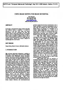
3.5 Extracting Shape and Location Features
In our FRIP system, we use two kinds of shape feature. For the global geometric shape feature, we first use eccentricity. Then for the local geometric feature, we modify the radiusbased shape signature (Modified Radius-based Signature: MRS) to be invariant under the shape’s scaling, rotation and translation. MRS is only applied to shapes that satisfy the eccentricity at the first step. Eccentricity is used to significantly reduce the amount of computation required for shape matching at run time. 3.5.1. Eccentricity for Global Shape Feature. To calculate eccentricity, we first estimate the bounding rectangle for each segmented region. From the major axis (Rmax) and the minor axis (Rmin), we can obtain the eccentricity at the similarity comparison step. Eccentricity (E) is defined as the ratio of Rmax to Rmin between query (Q) and target region (T): E=
RQmin RTmin − RQmax RTmax
|
|
(7)
3.5.2. MRS for Local Shape Feature. After calculation of the eccentricity, the centroid is calculated from each region. The location of each region is defined by this centroid (Cx, Cy). Here, the spatial location distance (dPQ,T) between two regions is measured by the Euclidean distance: dPQ,T = 冑(CxQ − CxT)2 + (CyQ − CyT)2
(8)
To estimate MRS, the boundary of a segmented region is extracted using Sobel edge detection and edge thinning
Region-based Image Retrieval
177
algorithms. After boundary extraction, a shape is represented by a feature function called a signature. Original signatures are invariant to translation, but they are sensitive to rotation and scaling. In our FRIP system, we modify the radius-based signature (MRS) to make it invariant to scaling and rotation, as well as translation. First, to achieve rotation invariance, we calculate the orientation of a region. Orientation () is defined as the angle of axis of the least moment of inertia [9]. From a given orientation, we create a central axis that passes through the centroid with the sloping of degrees. Then we estimate the starting point as the furthest point from the centroid to two symmetric boundary points aligned with the central axis. With this method, we can maintain the same starting point, even though the shape is somewhat distorted by its movement or occlusion. MRS is estimated from the starting point in the clockwise direction. However, because there are two MRSs about a starting point, we have to consider two different directional MRSs (clockwise and counterclockwise). To save storage space, we obtain and store only one MRS that is estimated from the starting point in the clockwise direction. To achieve scale invariance, we use a combination of MRS and Eq. (9). Equation (9) represents the differential variance between the average MRS ratio of the query region to a region in the database and individual MRS ratio: dMRS Q,T =
1 N
冘 冋冉 冘 | |冊 | |册 N
i=1
1 N
N
i=1
Qi Ti
−
Qi Ti
2
(9)
Image keys: imageNo { attribute int RegionNo; attribute int AverRed(AR); attribute int AverGreen(AG); attribute int AverBlue(AB); attribute int Normalised Area (NArea); attribute int CenterOfX(Cx); attribute int CenterOfY(Cy); attribute int MajorLength(Rmax); attribute int MinorLength(Rmin); attribute Array具int典 Signature[12]; attribute float AmplOfXDirect(Xd); attribute float AmplOfYDirect(Yd); }
4. STEPWISE SIMILARITY MATCHING In the FRIP system, the actual matching process is to search for the k elements in the stored region set closest to the query region. After regions are segmented, the user selects a region that he/she wants to search. Finally, using the userspecified constraints (such as (1) colour-care/don’t care, (2) scale (NArea)–care/don’t care, (3) shape–care/don’t care, (4) location–care/don’t care), the overall matching score is calculated according to Eq. (10). 4.1. Stepwise Distance Estimation
For example, if a database region and scale-up (or down) query region have similar shapes, two shape distances are calculated to be approximately zero. Therefore, the smaller one can be chosen as the real shape distance (dMRS Q,T ) between the query (Q) and the target MRS (T), even if the query region is rotated or translated. Here, to reduce the index size, we extract 12 radius (N) distance values with a 30 degree spacing and add these values to the region index. By using MRS and Eq. (9), our system is more robust against distortion, rotation and scale changes of a region, because they provide local information of shape with global information. Finally, we save 12 statistical properties of each region as an index to the database. All properties are shown below:
After feature normalisation, its associated weights are initialised to 1/q, where q is the dimension of the feature space. The system carries out image retrieval using K-nearest neighbour search based on the current weights to compute the similarity between the query region and database regions. It returns the top K nearest images, including similar regions. During the matching process, the following steps are taken to calculate the final score according to the user constraints: 1. At the first step, average colours (and eccentricity, in the case of shape–care) of the query region are only compared with regions in the database (Eqs (4),(7)). 2. If one (or two, in the case of shape–care) of the region
Fig. 2. Region signature. (a) Original image, (b) region boundary, (c) polygon by MRS.
178
B. Ko et al
distances between the query and the database is (are) below a threshold, the next distance calculation is permitted. By the first step, we can reduce the comparison time for shape matching significantly. 3. The directional texture distance is calculated using Eq. (5). 4. By the user’s choice, all or a few distances are calculated (Eqs (6), (8), (9)): + w4dTQ,T Score = w1dCQ,T + w2dPQ,T + w3dNArea Q,T
The relative relevance, as a weighting scheme, can then be given by
冒冘 q
wi(z) = (ri(z))t
where t = 1, 2, giving rise to linear and quadratic weightings, respectively. Finally, Eq. (14) can be changed following the exponential weighting scheme:
冒冘 q
wi(z) = exp(Tri(z))
+wd
(14)
l=1
(10)
MRS 5 Q,T
(rl(z))t
exp(Trl(z))
(15)
l=1
(w1 + w2 + w3 + w4 + w5 = 1) From the calculated distances, the final score is estimated (Eq. (10)), and the top k nearest images are displayed in ascending order of the final score.
5. MODIFIED PROBABILISTIC FEATURE RELEVANCE LEARNING (MPFRL) FOR FRIP’s MATCHING SCHEME In this section, we apply a new Probabilistic Feature Relevance Learning (PFRL) method to our FRIP system, with additional improvements (history concept and momentum term for weight updating) in order to improve the retrieval performance.
where T is a parameter that can be chosen to maximise (minimise) the influence of ri on wi. When T = 0, weight wi = 1/q, thereby ignoring any difference between the ri’s. On the other hand, when T is large, a change in ri will be exponentially reflected in wi. The exponential weighting is more sensitive to changes in local feature relevance (15), and gives rise to a better performance improvement. To estimate Eqs (14) and (15), one must first compute Eq. (13). The retrieved images with relevance feedback from a user can be used as training data to obtain estimates for Eq. (13), and hence Eqs (14) and (15). Let {xj, yj}k1 be the training data. Here xj denotes the feature vector representing the jth retrieved image, and yj is marked with either 1 (relevant) or 0 (irrelevant) by the user as the class label associated with xj. To compute E[f(x)兩xi = z], recall that f(x) = E[y兩x]. Thus, it follows that E[f兩xi = z] = E[y兩xi = z]
5.1. Probabilistic Feature Relevance Learning (PFRL) [5]
In a two class (1/0) classification problem, the class label c at query x is treated as a random variable from the distribution {Pr(1兩x), Pr(0兩x)}. The c at x can be characterised by y兩x =
再
1 c 兩x = 1
This gives rise to (11)
To predict c at x, f(x) is estimated from a set of training data. In image retrieval, however, the ‘label’ of x is known. All that is required is to exploit the differential relevance of input features to image retrieval. The least-squares estimate for f(x), given that x is known at dimension xi = z, is
冕
E[f兩xi = z] = f(x)p(x兩xi = z)dx
冒冘 K
yj1(兩xji − z兩ⱕ ⍀)
1(兩xji − z兩ⱕ ⍀)
(16)
j=1
where 1(·) is an indicator function. That is, 1(·) returns 1 if its argument is true, and 0 otherwise. ⍀ can be chosen so that there are sufficient data for the estimation of Equation (15), ⍀ can be chosen such that
冘 K
1(兩xji − z兩ⱕ ⍀) = C
(17)
j=1
where C ⱕ K is a constant. 5.2. Modified PFRL (MPFRL)
(12)
where p(x兩xi = z) is the density of other input features. Equation (12) shows the predictive strength (probability) when the value of just one (xi) of the input features is known. Then a feature relevance measure for query z can be given by ri(z) = E[f(x)兩xi = z]
冘 K
Eˆ[y兩xi = z] =
j=1
0 c 兩x ⫽ 1
f(x) = Pr(1兩x) = Pr(y = 1兩x) = E(y兩x)
However, since there may not be any data at xi = z, the data from the vicinity of xi at z are used to estimate E[y兩xi = z], a strategy suggested in Friedmon [6]. Therefore, Eq. (13) can be estimated according to
(13)
The original PFRL algorithm [5] is memoryless, in that retrieval in previous iterations does not contribute to feature relevance estimates in future iterations. As a result, retrieval performance may fluctuate from one iteration to the next, which might cause performance degradation. To overcome this limitation, we modify PFRL with two additional features. First, we add a momentum term to the weight update rule. That is, since the weights from a previous iteration
Region-based Image Retrieval
179
are also determined by the user’s perception, they include important attributes for predicting the weights for the next iteration. Furthermore, if we only use the weights estimated from the current user action, these may be dramatically changed or oscillated around the solution, so there may not be any increase in retrieval precision. By using this momentum term, we can prevent unstable changes of weights, and help to speed up learning. Secondly, we keep the user’s entire past feedback actions in order to improve performance for future iterations. If we are to ignore feedback actions from previous iterations, rejected images, which were selected as irrelevant in the past, may again be retrieved so that performance at the next iteration may not improve, in spite of an increase in the iteration time. Therefore, we use the previous relevance feedback as a history to help improve the performance and reduce the user’s time investment. Here, our history consists of two parts: one is the positive history, and the other is the negative history. The Modified Probabilistic Feature Relevance Learning (MPFRL) algorithm works in the following way. The first iteration is determined by weights initialised to (1/q). The resulting retrievals (images) are presented to the user using initial weights and Eq. (10). Then, the user marks the retrieved images (by clicking on them with a mouse) as either relevant or irrelevant, conditioned on their similarity to the desired target image. If the user does not know if a displayed image is similar to the desired target image, the user does not need to select that image. The user then presses the ‘Refinement’ button to adjust the weights for the next iteration. At this time, the new weights are estimated from the marked images using Eqs (16) and (15). In our experiments, we choose the parameter T (Eq. (15)), to be one. Then, these weights are updated by = (1 − ␣) · wti + ␣ · wt−1 wt+1 i i
(18)
where 0 ⱕ ␣ ⱕ 1 is an adjustable parameter that determines the extent to which the two terms should be combined, and t presents the iteration time. The next weight, wit⫹1, is updated by a linear combination of the weight of previous iteration, wit⫺1, and that from the current iteration, wti, by Eq. (15). After the weight update using Eq. (18), the next weight, wit⫹1, is used to carry out K-nearest neighbour search at the next iteration. To determine ␣, we calculate the average of the weight difference in the five features between iterations. To do so, we use our database images having a Sun region, because it preserves consistent shape, colour, texture, NArea and location. If we do not use ␣ (alpha 0), the difference graph is dramatically changed at every step, even though retrieval performance is good. If ␣ is 0.2 or 0.3 (alpha 2, 3), the difference graph is changed more slowly, but the retrieval performance is not superior to alpha being 0. On the contrary, if we choose ␣ to be 0.1 (alpha 1), the difference graph is changed slowly and retrieval performance is relatively superior to others. Therefore, in this paper, we select ␣ to be 0.1. During the K-nearest neighbour search step, we add a history scheme to the weighted similarity computation using Eq. (19). Here, history is generated by a user’s selection
Fig. 3. Cumulative distribution of weight difference (%: precision).
(action): at each iteration, if the user marks the k images as relevant or irrelevant, these images are recorded in the positive history HP = {h1(I1, P1), h2 (I2, P2), . . ., hi(Ii, Pi)} and negative history HN = {h1 (I1, N1), h2 (I2, N2), . . ., hi (Ii, Ni)}, respectively. if y 苸 HP{hi, %, hn}
冋冘 F
D(x, y) =
i=1
else if y 苸 HN{hi, %, hn}
冋冘 F
D(x, y) =
i=1
册
widi(fi(x), fi(y)) ·Kˆ (19)
册
widi(fi(x), fi(y)) ·Kˆ
In the above equation, x is an image including the query region, and y is a database image. HP {hi, %, hn} represents the set of relevant images, and HN {hi, %, hn} represents a set of irrelevant images. The distance (D) of feature vectors is estimated by a weighted sum of five distances (di, i: 1苲5– Eqs (4), (5), (6), (8), (9)), and Kˆ is a constant decision parameter for top k. In this paper, we set Kˆ to 10. At first, positive history (HP) checks whether the image y is included in HP or not. If y is included in HP, the distance between x and y is divided by the decision parameter Kˆ. On the other hand, if y is included in the negative history (HN), the distance is multiplied by parameter Kˆ. Here, if the iteration time is zero or an image is not included in any histories, the decision parameter Kˆ does not affect the distance. From the history scheme, we update the distance order between the query and a database region, and return the top k-nearest neighbour images, including similar regions. For example, if one image is selected as irrelevant at the previous iteration, it will get a larger distance (D) by Kˆ, and has a higher probability of being dropped from the top k images. On the other hand, if one image is selected as relevant, it will get a smaller distance (D) by Kˆ, and has a higher probability of being included in the top k images. This process is repeated until all of the desired images are found, or the predefined precision threshold is reached. The main steps of the modified probabilistic feature relevance learning algorithm are shown below:
180
B. Ko et al
Fig. 4. FRIP’s matching procedure using MPFRL.
1. Let i be the current query; initialise the weight vector w to {1/q}q1 2. Compute k nearest images using initial w and Eq. (10). 3. User marks n images as relevant or irrelevant. 4. Initiate history HP and HN. 5. While [(precision ⬍) or (user is not satisfied)] Do (a) Tset{marked n images}. (b) Estimate w from Eqs (15) and (16) using training data in Tset. (c) Update new weights from Eq. (18). (d) Compute k nearest images using new weights and history using Eq. (19). (e) User marks the n images as relevant or irrelevant. (f) Update history HP and HN.
6. EXPERIMENTAL RESULTS We have performed a variety of queries using a set of 3000 images from the WWW and Corel photo-CD, containing
various categories such as natural images (e.g. landscape, animals) and synthetic images (e.g. graphics, drawing). This system is developed in the Visual C⫹⫹ 6.0 language as an offline system. The average segmentation time requires approximately 30 seconds per image, and the average retrieval time requires 2 seconds per 1000 images using a Pentium PC, 450 MHz. The retrieval results are accessible at http://vip.yonsei.ac.kr/Frip. The experiments are carried out on eight specific domain data items, such as Sun, tiger, car, eagle, airplane and flower, between MPFRL with that of PFRL. First, a user chooses a query image and pushes the segment button. Then, the user selects k and ‘double clicks’ the region that he/she wants to retrieve. A user can choose colour, NArea (scale), shape and location (texture is included as a default condition) constraints in order to search regions more precisely. In this experiment, we chose all of the user constraints, and the top 18 nearest neighbours are returned that provide necessary relevance feedback. In all the experiments, the performance is measured using the average retrieval precision: precision =
Positive Retrievals Total Retrievals
(20)
Figure 6 shows the performance achieved by MPFRL and PFRL. Here we can see that the precision of PFRL is either stable or linearly increases or decreases in spite of the increased iteration time, but the precision of MPFRL never goes down, and improves steadily, because MPFRL uses the history concept. Figure 7 shows five weight changes on four categories as a function of iteration. Here, wi(i: 1苲5) is a weight for each of five features (colour, texture, NArea, shape and location). In Fig. 7, it can be seen that for all the queries, the weights associated with the relevant features are increased, and the
Fig. 5. User interface of FRIP system.
Region-based Image Retrieval
181
Fig. 6. Performance of eight specific regions between MPFRL and PFRL.
182
B. Ko et al
weights associated with the irrelevant ones are decreased after learning has taken place. These results show convincingly that our method can capture local feature relevance. Figures 8–11 show the top 10 retrieval results about the query region with corresponding segmented images.
Fig. 7. Weight changes of features according to the iteration.
Fig. 9. Retrieval results (query region: tiger–5 relevance feedback, top–10). Left is the original image, right is the segmented image.
Fig. 8. Retrieval results (query region: Sun–5 relevance feedback, top–10). Left is the original image, right is the segmented image.
Fig. 10. Retrieval results (query region: car–5 relevance feedback, top–10). Left is the original image, right is the segmented image.
Region-based Image Retrieval
183 Acknowledgement
The authors would like to thank the anonymous reviewers for their valuable comments.
References
Fig. 11. Retrieval results (query region: eagle–5 relevance feedback, top–10). Left is the original image, right is the segmented image.
7. CONCLUSION This paper presents a region-based image retrieval system, FRIP, that is able to tolerate, as for as possible, region scaling, rotation and translation, and which incorporates probabilistic feature relevance learning with two additional properties (history concept and weight momentum) to enable our system to perform region-based image retrieval in a desired manner. The experimental results using real image data show that our MPFRL algorithm can indeed rapidly improve the region-based retrieval performance of an image database system. Furthermore, since our relevance estimate is local in nature, the resulting retrieval, in terms of the shape of the neighbourhood, is highly adaptive and customised to the query location. A potential extension to the technique described in this paper is to consider additional derived variables (features) for local relevance estimates, thereby contributing to the distance calculation. The derived features are functions, such as linear functions, of the original features. When the derived features are more informative, huge gains may be expected. On the other hand, if they are not informative enough, they may cause retrieval performance to degrade, since they add to the dimensionality count. The challenge is to be able to have a mechanism that computes such informative-derived features efficiently.
1. Flickner FM, Niblack W, Petkovic D, Equitz W, Barber R. Efficient and effective querying by image content. Research Report #RJ 9203 (81511), IBM Almanden Research Center, San Jose, August 1993 2. Smith JR, Chang SF. VisualSEEk: A fully automated contentbased image query system. ACM Multimedia, Boston, MA, 1996 3. Ma WY, Manjunath BS. Netra: A toolbox for navigating large image database. IEEE International Conference on Image Processing, 1997 4. Thomas CM, Belongie S, Hellerstein JM, Malik J. Blobworld: A system for region-based image indexing and retrieval. Proc Int Conf Visual Inf Sys, 1999 5. Peng J, Bhanu B, Qing S. Probabilistic feature relevance learning for content-based image retrieval. Computer Vision and Image Understanding 1999; 75(1):150–164 6. Friedman JH. Flexible Metric Nearest Neighbor Classification. Technical Report, Department of Statistics, Stanford University, 1994 7. Ko B, Lee H-S, Byun H Region-based image retrieval system using efficient feature description. Proceedings of the 15th International Conference on Pattern Recognition 2000; 4(4):283–286 8. Burrus S, Gopinath RA, Guo H. Introduction Wavelets and Wavelet Transforms. A primer. Prentice-Hall, 1998 9. Jain AK. Fundamentals of Digital Image Processing. Prentice Hall, 1989 10. Ciocca G, Schettini R. A relevance feedback mechanism for content-based image retrieval. Information Processing and Management 1999; 3:605–632 11. Rui Y, Huang TS, Mehrotra S. Content-based image retrieval with relevance feedback in MARS. IEEE International Conference on Image Processing, Santa Barbara, CA, October 1997; 815–818 12. Rui Y, Ortega TSM, Mehrotra S, Relevance feedback: a power tool for interactive content-based image retrieval. IEEE Trans Circuits and Systems for Video Technology 1998; 2(5):644–655 13. Cox IJ, Miller ML, Minka TP et al An optimized interaction strategy for Bayesian relevance feedback. Proceedings of IEEE CVPR’98, Santa Barbara, CA, 1998 14. Nastar C, Mitschke M, Meihac C. Efficient query refinement for image retrieval. Proceedings of IEEE CVPR’98, Santa Barbara, CA, 1998 15. Aggarwal G, Dubey P et al iPURE: Perceptual and user-friendly retrieval of images. Proceedings of IEEE International Conference on Multimedia and Expo 2000; 3(2):693–696
ByoungChul Ko received his BS degree from Kyonggi University, Korea, in 1998, and MS degree from Yonsei University, Korea, in 2000, both in computer science. He is currently a PhD student in the Department of Computer Science, Yonsei University, Korea. His research interests include multimedia information retrieval, computer vision, gesture recognition and statistical pattern recognition. He received the excellent paper award in 2000 from the Korea Information Science Society.
Jing Peng received his MA in computer science from Brandeis University, and PhD in computer science from Northeastern University, Boston, in 1994. He
184 also received a BS in computer science from the Beijing Institute of Aeronautics and Astronautics, Beijing, China. Since 1999, he has been an assistant professor of Computer Science at Oklahoma State University. Previously, he was a research scientist at the Center for Research in Intelligent Systems at the University of California at Riverside. Dr Peng’s research interests include machine learning, pattern classification, image databases, data mining and learning and vision applications.
Hyeran Byun received her BS and MS degrees in mathematics from Yonsei University, Korea. She received her PhD in computer science from Purdue
B. Ko et al University, West Lafayette, Indiana. She was an assistant professor in Hallym University, Chooncheon, Korea from 1994–1995. Since 1995 she has been an associate professor of Computer Science at Yonsei University, Korea. Her research interests are in multimedia, computer vision, image and video processing, artificial intelligence and pattern recognition.
Correspondence and offprint requests to: B Ko, VIP Lab, Department of Computer Science, Yonsei University, Shinchon-Dong, Seodaemun-Gu 120–749, Korea. Email: soccer1얀aipiri.yonsei.ac.kr