Region Proximity in Metric Spaces and Its Use for ... - CiteSeerX

Region Proximity in Metric Spaces and Its Use for Approximate Similarity Search GIUSEPPE AMATO, FAUSTO RABITTI, and PASQUALE SAVINO ISTI-CNR and PAVEL ZEZULA Masaryk University

Similarity search structures for metric data typically bound object partitions by ball regions. Since regions can overlap, a relevant issue is to estimate the proximity of regions in order to predict the number of objects in the regions’ intersection. This paper analyzes the problem using a probabilistic approach and provides a solution that effectively computes the proximity through realistic heuristics that only require small amounts of auxiliary data. An extensive simulation to validate the technique is provided. An application is developed to demonstrate how the proximity measure can be successfully applied to the approximate similarity search. Search speedup is achieved by ignoring data regions whose proximity to the query region is smaller than a user-defined threshold. This idea is implemented in a metric tree environment for the similarity range and “nearest neighbors” queries. Several measures of efficiency and effectiveness are applied to evaluate proposed approximate search algorithms on real-life data sets. An analytical model is developed to relate proximity parameters and the quality of search. Improvements of two orders of magnitude are achieved for moderately approximated search results. We demonstrate that the precision of proximity measures can significantly influence the quality of approximated algorithms. Categories and Subject Descriptors: E.1 [Data Structures]: Trees; E.5 [Files]: Sorting-searching; H.2.2 [Database Management]: Physical Design—Access methods; H.3.3 [Information Storage and Retrieval]: Information Searching and Retrieval—Search process General Terms: Algorithms, Performance Additional Key Words and Phrases: Approximation algorithms, performance evaluation, metric trees, approximate similarity search, metric data

1. INTRODUCTION In traditional database systems with attribute data, queries are typically executed by searching for records which exactly match the query. On the other hand, the standard approach for exploring modern data repositories, such as multimedia databases, is to do a search on features extracted from complex Authors’ addresses: G. Amato, F. Rabitti, and P. Savino: ISTI-CNR, Via G. Moruzzi 1, 56124 Pisa, Italy; email: (Amato,Rabitti,Savino)@isti.cnr.it; P. Zezula, Faculty of Informatics, Masaryk University of Brno, Botanicka 68a, 602 00 Brno, Czech Republic; email: [email protected]. Permission to make digital/hard copy of part or all of this work for personal or classroom use is granted without fee provided that the copies are not made or distributed for profit or commercial advantage, the copyright notice, the title of the publication, and its date appear, and notice is given that copying is by permission of ACM, Inc. To copy otherwise, to republish, to post on servers, or to redistribute to lists requires prior specific permission and/or a fee. ° C 2003 ACM 1046-8188/03/0400-0192 $5.00 ACM Transactions on Information Systems, Vol. 21, No. 2, April 2003, Pages 192–227.

Region Proximity in Metric Spaces

•

193

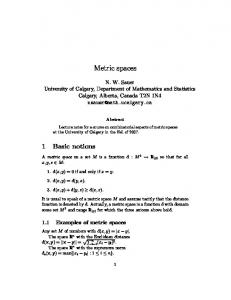
information objects. Features are typically defined in high-dimensional vector spaces or even generic metric spaces where pairs of elements can only be compared by distance functions. Considering such data, exact match has little meaning, and thus concepts of similarity are typically applied. From a formal point of view, the mathematical notion of metric space (see, for example, Kelly [1955]) provides a useful formalization of similarity or nearness. In this article, we assume objects to be elements of a metric space. Similarity searches have become fundamental in a variety of application areas, including multimedia information retrieval, data mining, pattern recognition, machine learning, computer vision, genome databases, data compression, and statistical data analysis. This problem was originally studied by the computational geometry community, where it is known as the closest point, nearest neighbor, or post office problem. However, it has recently attracted much attention in the database community, because of the increasingly growing need to deal with large volumes of data. Consequently, efficiency has become a matter of importance. Although a lot of work has been done to develop structures which are able to perform similarity searches quickly, the results are still not satisfactory, and much more research is needed. The necessary starting point to implement a similarity search algorithm is to consider a measurable distance (dissimilarity), which in turn allows objects to be ranked according to their distance with respect to a given reference (target or query) object. Similarity queries are defined by a query object and a constraint on the ranked list of data objects, which is typically specified as a distance threshold or a number of required objects. In any case, a query can be seen as a ball region and the qualifying objects are those that are contained in (or covered by) this region. In order to speed up retrieval in large collections of metric data, access methods have been developed. An excellent survey of methods for vector spaces can be found in Gaede and Gunther [1998], while a comprehensive list of techniques ´ for generic metric spaces is analyzed in Chavez et al. [2001]. The common underlying principle of such access methods is to divide searched data sets into partitions, and bound such partitions by regions. These partitions are stored in storage buckets (tree nodes, pages, or blocks of data). When a query is issued, only buckets corresponding to regions that overlap the query region need to be examined. This reduces the bucket access costs as well as the distance computation costs, since the number of distance computations is proportional to the number of accessed buckets. Contrary to partitions containing disjoint sets of objects, the partitions’ bounding regions can overlap. Consider the example in Figure 1 where data objects are divided into three partitions, distinguished by the white, black, and gray points, and bounded, respectively, by regions R1 , R2 , and R3 . Objects qualifying for a query region Q are retrieved by accessing partitions whose corresponding regions intersect Q. Although many proposals exist, access methods do not always perform well, as confirmed by theoretical studies [Beyer et al. 1999; Weber et al. 1998] conducted for vector spaces. When the probability of overlap between the query and data regions becomes high, the execution of a similarity query requires access ACM Transactions on Information Systems, Vol. 21, No. 2, April 2003.

194

•

Amato et al.

Fig. 1. Data partitions, data regions, and query regions.

to many data regions and partitioning is not actually useful. For instance, in Figure 1, the query region overlaps regions R1 , R2 , and R3 , so all of them should be accessed to answer the query. The number of data objects contained in the intersections depends on the distribution of data objects. There may be regions with a large intersection and few objects in common, but also regions with a small intersection and many objects in common, which happens when the intersection covers a dense area of the data object space. In this paper, we refer to this phenomenon as the proximity of regions and develop techniques for its quantification. The problem of region proximity in vector spaces was studied in Kamel and Faloutsos [1992] to decluster nodes of R-trees [Guttman 1984] for parallelism. In this paper, we develop proximity measures for general metric spaces, which naturally subsumes the case of vector spaces. We propose a technique with the objective of satisfying the following criteria: (1) the proximity is measured with sufficient precision; (2) the computational costs are low; (3) the approach can be applied to different metrics and data sets; (4) storage overheads are moderate. In this paper, we analyze the problem of the proximity of regions in metric spaces using a probabilistic approach. We validate the proposed technique by designing approximate search algorithms for the similarity range and the “nearest neighbors” queries that exploit the proximity measure. We develop an analytical model and perform extensive experimental evaluations, which demonstrate big improvements in retrieval efficiency. We also show that the precision of the proximity measure is fundamental for achieving a high-quality approximation. The rest of the paper is organized as follows. In Section 2 we present the necessary background. Section 3 discusses the proximity measure and its effective and efficient computation. In Section 4 we validate the proposed approaches. In Section 5 we introduce the problem of approximate similarity retrieval and apply the proximity measure to this problem. Results of the approximated similarity search are presented in Section 6. Section 7 compares our approach to an approximate similarity search with previous designs. Conclusions are drawn in Section 8. ACM Transactions on Information Systems, Vol. 21, No. 2, April 2003.

Region Proximity in Metric Spaces

•

195

2. PRELIMINARIES This section provides definitions of basic terms used in this article. In particular, we introduce metric spaces, present examples of distance functions, and define the notion of distance distribution. 2.1 Metric Spaces A metric space M = (D, d ) is defined by a domain of objects D and by a total (distance) function d , which satisfies for each triple of objects Ox , O y , Oz ∈ D the following properties: (1) (2) (3) (4)

d (Ox , O y ) = d (O y , Ox ) 0 < d (Ox , O y ) < ∞, Ox 6= O y d (Ox , Ox ) = 0 d (Ox , O y ) ≤ d (Ox , Oz ) + d (Oz , O y )

(symmetry) (nonnegativity) (identity) (triangle inequality)

We assume that the maximum distance never exceeds d m ; thus we consider a bounded metric space. Given the metric space M, we define a ball region Bx as Bx = Bx (Ox , rx ) = {Oi ∈ D | d (Ox , Oi ) ≤ rx } A ball region Bx is determined by a center Ox ∈ D and a radius rx ≥ 0. It includes objects from D with distances to Ox smaller than or equal to rx . 2.1.1 Metric Functions. The traditional way of measuring distances in vector spaces is to use a Minkowski-form distance. This set of distance measures is often designated as the L p distance and it is defined for vectors vx and v y as  1/ p n X | vx [ j ] − v y [ j ] | p  , p ≥ 1, (1) L p (vx , v y ) =  j =1

with L1 known as the city-block or Manhattan distance, and L2 the Euclidean distance. L p considers vector coordinates to be independent; thus distances are proportional to the closeness of vectors in a multidimensional space. However, vector coordinates can be dependent or correlated and this natural (though also subjective) cross-talk of dimensions should be taken into account [Faloutsos 1996]. One way to approach this problem is to use the quadratic-form distance 2 (vx , v y ) = (vx − v y )T A(vx − v y ), d qf

(2)

where A = [ai, j ] is a correlation matrix between dimensions of vectors vx and v y , and the superscript T indicates the vector transposition. This measure satisfies the metric postulates, provided the matrix is symmetric and ai,i = 1. Another example of a metric measure is the Levenshtein (also called the edit) distance to quantify similarity over strings. It is defined as the minimal number of string symbols that have to be inserted, deleted, or substituted to transform a string Ox into a string O y ; see, for example, Hall and Dowling [1980]. ACM Transactions on Information Systems, Vol. 21, No. 2, April 2003.

196

•

Amato et al.

Similarity of sets, also called the Jacard’s coefficient, is a measure that applies to nonvector data. Given two sets A and B, the similarity is defined as the ratio of the number of their common elements to the number of all different elements #(A ∩ B) , (3) ST (A, B) = #(A ∪ B) where #(C) is the number of elements in set C. Note that 1 − ST (A, B) is a metric distance function. A generalization of this measure is the Tanimoto similarity measure [Kohonen 1984] ST (vx , v y ) =

(vx , v y ) , kvx k2 + kv y k2 − (vx , v y )

(4)

which is defined for vectors with (vx , v y ) being the scalar product of vx and v y , and kvx k the Euclidean norm of vx . As a final example, consider the Hausdorff distance, which is used to compare shapes of images [Huttenlocker et al. 1993]. Here the compared objects are sets of relevant, for example high-curvature, points. 2.2 A Note on Distance Distribution Let D O be a continuous random variable corresponding to the distance d (O, O1 ), where O1 is a random object. The distance density f DO (x) represents the probability1 of distance x from object O. The corresponding distance distribution F DO (x) is the probability that a distance to O does not exceed x, which can be determined as Z x f DO (t) dt. (5) F DO (x) = 0

Given two different objects Ox , O y ∈ D, the corresponding distance distributions F DOx and F DO y are different functions. We can also say that F DOi represents the Oi ’s point of view of the domain D. However, it is not feasible to compute and maintain distance distributions with respect to all objects from D. An alternative solution may be to consider an overall distribution of distances over D. This can be defined as F (x) = Pr{d (O1 , O2 ) ≤ x},

(6)

where O1 and O2 are two independent random objects of D. The use of F (x) instead of F DO (x) has been investigated and justified in Ciaccia et al. [1998], where numerous synthetic and real-life files were tested. For all these data sets, the difference in using F (x) in place of F DO (x) was negligible. However, even if we neglect the computational complexity of a procedure that would be able to determine F (x), all objects from D are usually not known. In 1 We

are using continuous random variables, so, to be rigorous, the probability that they take a specific value is by definition zero. However, in order to simplify the explanation, we slightly abuse the terminology and use the term probability to give an intuitive idea of the behavior of the density function being defined.

ACM Transactions on Information Systems, Vol. 21, No. 2, April 2003.

Region Proximity in Metric Spaces

•

197

such cases, we compute an estimation of F (x), by considering distances between objects from a representative sample of D. 3. PROXIMITY Intuitively, the proximity of two ball regions is proportional to the number of objects that simultaneously occur in both of the regions. We define the proximity X (Bx , B y ) of ball regions Bx , B y as the probability that a randomly chosen object O ∈ D appears in both regions, that is: X (Bx , B y ) = Pr{d (O, Ox ) ≤ rx ∧ d (O, O y ) ≤ r y }.

(7)

Note that the proximity cannot be quantified by the amount of space covered by the regions’ intersection. Due to the lack of space coordinates in general metric spaces, such a quantity cannot be determined. In existing applications, such as Ciaccia et al. [1997] and Traina et al. [2000], a simplified measure of the proximity between two ball regions is used. Specifically, the proximity is computed through a function, linearly proportional to the overlap of the regions, which can be generalized as follows:  0, if rx + r y < d (Ox , O y ),    r + r − d (O , O ) x y x y trivial , if max(rx , r y ) ≤ min(rx , r y ) + d (Ox , O y ), (Bx , B y ) = X 2 · d m − d (Ox , O y )    2 · min(rx ,r y ) , otherwise. (8) 2 · d m − d (Ox , O y )

Equation (8) sets the proximity to zero when two ball regions do not overlap. The values are normalized to obtain proximity values in the range [0,1]. The proximity is 1 when both regions include all objects, that is when their radii are equal to the maximum distance d m . Although this proximity measure is simple to compute, it is not accurate because it does not take into account the distribution of objects in the space. As we discuss in Section 3.1 and verify later, the issue of proximity is far more complex. 3.1 Computational Difficulties of the Proximity Measure To precisely compute proximity according to Equation (7), the knowledge of distance distributions with respect to the regions’ centers is required. Since any object from D can become a region’s center, such knowledge is not likely to be obtained. As discussed in Section 2.2, we can assume, however, that the distribution depends on the distance between the regions’ centers, while it is (practically) independent of the centers themselves. This also implies that all pairs of regions with the same radii and constant distance between centers have on average the same proximity, no matter what their actual centers are. Consequently, we can approximate the proximity X (Bx , B y ) with the overall proximity Xdxy (rx , r y ) of pairs of regions having radii rx and r y , and whose distance between centers is d xy . Specifically, X (Bx , B y ) ≈ Xdxy (rx , r y ) = Pr{d (O, Ox ) ≤ rx ∧ d (O, Oy ) ≤ r y | d (Ox , Oy ) = d xy },

(9)

where Ox , Oy , and O are random objects. ACM Transactions on Information Systems, Vol. 21, No. 2, April 2003.

198

•

Amato et al.

Now, consider how Xdxy (rx , r y ) can be computed. Let X , Y , and DXY be continuous random variables corresponding, respectively, to distances d (O, Ox ), d (O, Oy ), and d (Ox , Oy ). The joint conditional density f X ,Y |DXY (x, y|d xy ) is the probability that distances d (O, Ox ) and d (O, Oy ) are, respectively, x and y, given that d (Ox , Oy ) = d xy . Then, Xdxy (rx , r y ) can be computed as Z rx Z r y f X ,Y |DXY (x, y|d xy ) dy dx. (10) Xdxy (rx , r y ) = 0

0

Unfortunately, an explicit form of f X ,Y |DXY (x, y|d xy ) is unknown. In Amato et al. [2000b], an analytic approach for obtaining proximity for a two-dimensional vector space is developed. However, the resulting computational costs, even for two dimensions, are too high for practical applications, and an extension to other metric spaces proved to be difficult. In addition, computing and maintaining joint conditional densities as discrete functions would result in a very high number of values. The function depends on three arguments so that the required storage space is O(n3 ), provided n is the number of samples used for each argument. This makes the approach totally unacceptable. We propose to compute the proximity measure using an approximation of appr f X ,Y |DXY (x, y|d xy ), designated as f X ,Y |DXY (x, y|d xy ), that is expressed in terms of the joint density f XY (x, y). Note that f XY (x, y) is simpler to determine than f X ,Y |DXY (x, y|d xy ). Since X and Y are independent random variables, f XY (x, y) = f X (x)· f Y ( y). Given the definition of the random variables X and Y , it is easy to show that f X (d ) = f Y (d ), so we can omit the name of the random variable and designate the joint density as f (d ). Such a density can be easily obtained by sampling from the data set. A preliminary version of this idea is published in Amato et al. [2000c]. The storage cost of this approach is acceptable, but the problem is how to transform the joint density into the joint conditional density. In the following, we put forward and investigate approximations that satisfy efficiency requirements and guarantee good quality results. 3.2 Effective and Efficient Proximity Measures Given objects Ox and O y with d (Ox , O y ) = d xy , the space of possible distances x = d (O, Ox ) and y = d (O, O y ), measured from an object O ∈ D, is constrained by the following triangular inequalities: x+ y ≥ d xy , x+d xy ≥ y, and y +d xy ≥ x. Figure 2 helps to visually identify these constraints. In the gray area, called the bounded area, the triangular inequality is satisfied, while in the white area, called the external area, the triangular inequality is not satisfied, so an object O with such distances to Ox and O y does not exist in D. In general, f X ,Y |DXY (x, y|d xy ) 6= f XY (x, y), because the joint density f XY (x, y) gives the probability that the distances d (O, Ox ) and d (O, Oy ) are x and y, no matter what the distance is between Ox and Oy . The difference between the two densities is immediately obvious when we consider the metric space postulates. Accordingly, f X ,Y |DXY (x, y|d xy ) is zero if x, y, and d xy do not satisfy the triangular inequality, because such distances simply cannot exist. However, f XY (x, y) is not restricted by such a constraint, and any pair of distances ACM Transactions on Information Systems, Vol. 21, No. 2, April 2003.

Region Proximity in Metric Spaces

•

199

Fig. 2. Area bounded by the triangular inequality.

0.00000025

0.00000025

0.000000225

0.000000225

0.0000002

0.0000002

0.000000175

0.000000175

0.00000015

0.00000015

0.000000125

0.0000001

0.0000001

0.000000075

0.000000075

Joint conditional density

y=5670

y=6370

y=4270

y=4970

y=2870

y=3570

y=1470

y=70

0 y=2170

y=5670

y=6370

y=4270

y=4970

y=2870

y=3570

y=1470

y=2170

y=70

y=770

0

70 70 0 x= 7 7 0 x= =14 17 0 x =2 87 0 x =2 57 0 x =3 27 0 x 4 7 x= =49 670 0 x =5 37 x =6 x

0.00000005 0.000000025

70 0 0 x= 77 47 0 x= =1 17 70 x =2 8 0 x =2 57 0 x =3 27 0 x 4 7 x= =49 670 0 x =5 37 x =6 x

0.00000005 0.000000025

y=770

0.000000125

Joint density

Fig. 3. Comparison between f X ,Y |DXY (x, y|d xy ) and f XY (x, y).

≤ d m is possible. To illustrate this, Figure 3 shows the joint conditional density f X ,Y |DXY (x, y|d xy ) for a fixed d xy and the joint density f XY (x, y). Note that the graph of the joint conditional density has values greater than zero only in the bounded area, and that quite high values are located near the edges. On the other hand, the joint density has values greater than zero also outside the bounded area. The graphs in Figure 3 are obtained using a two-dimensional uniformly distributed data set described in Section 4.1. These observations form the basis of our heuristics to obtain the approximate appr joint conditional density f XY|DXY (x, y|d xy ) by means of the joint density. The idea is to move f XY (x, y) densities from the external area into the bounded area. When distances x, y, and d xy satisfy the triangular inequality, the value of appr f XY|DXY (x, y|d xy ) depends on the specific strategy used to implement the previous appr idea; otherwise, f XY|DXY (x, y|d xy ) = 0. In this way, the integral over the bounded area is 1. This is the basic assumption of any probabilistic model that would be violated if the joint densities were simply trimmed off by the triangle inequality constraints. ACM Transactions on Information Systems, Vol. 21, No. 2, April 2003.

200

•

Amato et al.

Fig. 4. The four heuristics proposed to compute region proximity.

We have tried four different implementations of this heuristic, varying the strategy applied to move density values. Figure 4 provides a visual representation of the methods, where the circles represent the joint density function, while the arrows indicate directions in which the necessary quantities are moved from the external area to the bounded area. The strategies can be briefly characterized as follows. Orthogonal approximation. Collect points outside the bounded area and move them on top of the corresponding constraint following a direction that is orthogonal to the constraint. Parallel approximation. Collect points outside the bounded area and move them on top of the corresponding constraint following a direction that is parallel to the axis. Diagonal approximation. Collect points outside the bounded area and move them on top of the corresponding constraint following a direction that always passes through d m . Normalized approximation. Collect points outside the bounded area in order to determine a linear coefficient that modifies (increases) densities inside the bounded area. ACM Transactions on Information Systems, Vol. 21, No. 2, April 2003.

Region Proximity in Metric Spaces

•

201

Observe that for efficiency reasons, the proximity based on the orthogonal, parallel, and diagonal methods can be computed directly from the joint density f X ,Y (x, y) by integrating in the gray marked area, as illustrated in Figure 4. In this way, instead of moving densities to obtain the joint conditional density, the integration area is extended so that values of the joint density in the external area are considered as well. Specifically, Z bx (dxy ,rx ,r y ) Z b2y (x,dxy ,rx ,r y ) appr f X ,Y (x, y) dy dx. (11) X dxy (rx , r y ) = b1y (x,d xy ,rx ,r y )

0

In the following, we simplify the terminology by omitting the d xy , rx , and r y parameters in the integration bounds and use only the symbols bx (), b1y (x), and b2y (x). The integration bounds bx (), b1y (x), and b2y (x) are functions that are specific for each approximation method. The function bx () gives the integration range along the x axis, while b1y (x) and b2y (x) form the lower and upper bounds of the gray area along the y axis for a specific x. The normalized technique is even more simple because we only integrate in the bounded area restricted by the region radii (see the gray marked area in Figure 4) and we multiply the result by the normalization coefficient NC(d xy ) = 1/(1 − E(d xy )), where E(d xy ) is the integral of f XY (x, y) over the external area. A definition of the bounding functions bx (), b1y (x), and b2y (x) for all the methods does not present any particular mathematical complexity and is omitted here for the sake of brevity. A detailed specification can be found in Amato et al. [2000b] and Amato [2002]. 3.2.1 Computational Complexity. The computational cost of Equation (11) is clearly O(n2 ), where n is the number of samples needed for one integration. Since one of our major objectives is efficiency, such a cost is still high. However, we can transform the formula as follows: Z bx () Z b2y (x) Z bx () Z b2y (x) f XY (x, y) dy dx = f (x) f ( y) dy dx 0

b1y (x)

b1y (x)

0

Z =

0

bx ()

¡ ¡ ¢ ¡ ¢¢ f (x) · F b2y (x) − F b1y (x) dx. (12)

Provided the f (d ) and F (d ) functions are explicitly maintained in the main memory, Equation (12) can be computed with complexity O(n). This assumption is realistic even for quite high values of n, so the computational complexities of the orthogonal, parallel, and diagonal methods are linear. As far as the normalized method is concerned, we can see that the normalization coefficient is not restricted by specific region radii, and thus only depends on d xy . Such information can also be maintained in the main memory. Consequently, the computational complexity of the normalized method is also O(n). 4. VALIDATING THE APPROACHES TO THE PROXIMITY MEASURE In this section, we investigate the accuracy of the proposed approaches for computing the proximity. Before presenting the simulation results, we first ACM Transactions on Information Systems, Vol. 21, No. 2, April 2003.

•

202

Amato et al. HV1 Dataset 3.50E-04

2.50E-04

3.00E-04

HV2 Dataset 1.20E+00 1.00E+00

1.50E-04 1.00E-04

Density

2.50E-04

2.00E-04

Density

Density

UV Dataset 3.00E-04

2.00E-04 1.50E-04 1.00E-04

5.00E-05

0.00E+00 0

2000

4000 Distance

(a)

6000

8000

6.00E-01 4.00E-01 2.00E-01

5.00E-05

0.00E+00

8.00E-01

0.00E+00

0

2000

4000

6000

8000

0

0.5

Distance

(b)

1

1.5

2

Distance

(c)

Fig. 5. Distance density functions of the data sets used for the experiments.

characterize the data sets used to validate the approaches, describe the evaluation process, and define comparison metrics. 4.1 Data Sets We conducted our experiments using three data sets: one synthetic and two real-life data sets of image color features. The synthetic data set, called UV, is a set of vectors uniformly distributed in a two-dimensional space where vectors are compared through the Euclidean (L2 ) distance. The second data set, designated as HV1, represents color features of images. In this case, the features are represented as nine-dimensional vectors containing the average, standard deviation, and skewness of pixel values for each of the red, green, and blue channels [Stricker and Orengo 1995]. An image is divided into five overlapping regions, each one represented by a nine-dimensional color feature vector. This results in a 45-dimensional vector as a descriptor of one image. The distance function to compare two feature vectors is again the Euclidean (L2 ) distance. The third data set, called HV2, contains color histograms represented in 32 dimensions. This data set was obtained from the UCI Knowledge Discovery in Databases Archive [Hettich and Bay 1999]. The color histograms were extracted from the Corel image collection as follows: The HSV space is divided into 32 subspaces (colors), using eight ranges of hue and four ranges of saturation. The value for each dimension of a vector is the density of each color in the entire image. The distance function used to compare two feature vectors is the histogram intersection implemented as L1 . Data sets UV and HV1 contain 10,000 objects, while HV2 contains 50,000 objects. The distance density functions of all our data sets can be seen in Figure 5. Observe the differences in densities of the individual data collections that were selected to test proximity for qualitatively different metric spaces, that is, spaces characterized by different data (distance) distributions. 4.2 Experiments and Comparison Measures (rx , r y ) for all data sets as follows: We We computed the actual proximity Xdactual xy uniformly chose 100 values of d xy , rx , and r y in the range of possible distances. (rx , r y ) was computed for all possible combinations of the The proximity Xdactual xy chosen values. To accomplish this task, we found for each d xy 400 pairs of objects (Ox , O y ), that is, the centers of the balls, such that |d (Ox , O y ) − d xy | ≈ 0. For each pair of objects, we used the predefined values of rx and r y to generate ACM Transactions on Information Systems, Vol. 21, No. 2, April 2003.

Region Proximity in Metric Spaces

•

203

ball regions. Then, we only considered pairs of intersecting regions, because nonintersecting balls have 0 proximity and no verification is needed. For each pair of balls, we counted the number of objects in their intersection. The actual proximity was finally obtained by computing the average number of objects in the intersection for each generated configuration of d xy , rx , and r y and by normalizing (dividing by the total number of objects in the data set) such values to obtain the probability. We did not consider distances d xy of very low densities, because it was not possible to compute the actual proximity with sufficient precision—the data sets contained only very few objects at such distances. Once the actual proximity was determined, we computed the approximate proximity for the same values of d xy , rx , and r y . The comparison between the actual and the approximate proximity was quantified for each possible configuration as the absolute error ¯ ¯ appr (rx , r y ) − Xdxy (rx , r y )¯. ²(rx , r y , d xy ) = ¯ Xdactual xy An alternative way to evaluate our approaches would be to use the relative error, defined as the ratio of the absolute error and the actual proximity. However, our choice for the absolute error can be justified as follows. Suppose that the actual proximity is almost zero (e.g., 10−5 ), while the approximate proximity is exactly zero. In this case, the relative error is 1, that is, we have a high error. Consider now the opposite case where the actual proximity is zero, and our approximation is 10−5 . In this case, the relative error is ∞. However, given the meaning of proximity (see Section 1), and considering previous examples, we can say that such an approximation is good, because it almost gives the correct results. This means that the absolute error is a more objective measure, that is, more suitable for our purposes. Given the large number of experiments, we summarized the results by computing the average error ²µ0 (d xy ) for all pairs of radii at a given distance between the centers, and the average error ²µ00 (rx , r y ) for all distances between the ball centers at a given pair of radii, specifically: ²µ0 (d xy ) = Avgrx ry (²(rx , ry , d xy )) and ²µ00 (rx , r y ) = Avgdxy (²(rx , r y , dxy )). In a similar way, we computed the variance of the error for a given distance d xy : ²σ0 (d xy ) = Varrx ry (²(rx , ry , d xy )). The evaluation of ²µ0 is used to measure the average error of approximations for specific distances between the ball centers. However, ²µ0 alone is not sufficient to correctly judge the quality of the approximation. In fact, it is obtained as the average error for all possible values of rx and r y so that some peculiar behaviors may remain hidden. In this respect, the stability of the error must also be considered. For this purpose, we computed the variance ²σ0 . Note that high average errors and small variances may also provide good approximations. To illustrate this, suppose that we want to use the proximity to order (rank) a set of regions with respect to a reference region. The ranking results obtained ACM Transactions on Information Systems, Vol. 21, No. 2, April 2003.

•

204

Amato et al. UV dataset: variance of errors

UV dataset: average error

ε ,µ

1.40E-01

ε

1.20E-01

1.40E-02

,

σ

1.20E-02

1.00E-01

1.00E-02 Normalised Orthogonal Parallel Diagonal Trivial

8.00E-02 6.00E-02

Normalised Orthogonal Parallel Diagonal Trivial

8.00E-03 6.00E-03 4.00E-03

4.00E-02 2.00E-02

2.00E-03

0.00E+00 700

0.00E+00 700

1700

2700

3700

4700

1700

2700

dxy

dxy

3700

4700

HV1 dataset: average error

ε ,µ

1.80E-01

HV1 dataset: variance of errors

1.60E-01

1.60E-02

ε ,σ 1.40E-02

1.40E-01 1.20E-01

1.20E-02

Normalised Orthogonal Parallel Diagonal Trivial

1.00E-01 8.00E-02 6.00E-02

Normalised Orthogonal Parallel Diagonal Trivial

1.00E-02 8.00E-03 6.00E-03 4.00E-03

4.00E-02 2.00E-02

2.00E-03

0.00E+00 1000

0.00E+00 1000

2000

3000

dxy

4000

5000

6000

2000

HV2 dataset: average error

ε ,µ

3000

4000

5000

dxy

6000

HV2 dataset: variance of errors

3.00E-01

ε

2.50E-01

,

2.50E-02

σ 2.00E-02

2.00E-01

Normalised Orthogonal Parallel Diagonal Trivial

1.50E-01 1.00E-01

Normalised Orthogonal Parallel Diagonal Trivial

1.50E-02 1.00E-02 5.00E-03

5.00E-02 0.00E+00 0.4

0.6

0.8

1

1.2

1.4

1.6

0.00E+00 0.4

dxy

0.6

0.8

1

1.2

1.4

1.6

dxy

Fig. 6. Average and variance of errors given d xy .

through the actual and approximate proximity may turn out to be identical even though ²µ0 is quite high. In fact, when the variance of error is very small, it means that the error is almost constant, and the approximation somehow follows the behavior of the actual proximity. In this case, it is highly probable that the approximated proximity increases (or decreases) according to the trend of the actual one, thus guaranteeing the correct ordering. On the other hand, ²µ00 represents the average error from a different point of view and complements ²µ0 . It is determined for a given pair of radii (rx , r y ) by varying d xy . This measure offers a finer grained view on the error, since the average is only computed varying the distance d xy . 4.3 Observations on the Results Obtained For all data sets, the actual proximity was compared with our techniques and the trivial proximity (defined by Equation (8)). Figure 6 presents the average ACM Transactions on Information Systems, Vol. 21, No. 2, April 2003.

Region Proximity in Metric Spaces HV2: Trivial method

y=2.037 y=1.533 y=1.029 y=0.525 y=0.021 x=2.037

x=1.365

x=1.701

x=0.693

x=1.029

x=0.021

x=0.357

x=1.785

x=2.079

x=1.197

x=1.491

x=0.609

x=0.903

x=0.021

x=0.315

205

HV2: Parallel method

4.50E-01 4.00E-01 3.50E-01 ,, 3.00E-01 ε µ 2.50E-01 2.00E-01 1.50E-01 1.00E-01 y=2.037 5.00E-02 y=1.533 0.00E+00 y=1.029 y=0.525 y=0.021

4.50E-01 4.00E-01 3.50E-01 ,, 3.00E-01 ε µ 2.50E-01 2.00E-01 1.50E-01 1.00E-01 5.00E-02 0.00E+00

•

Fig. 7. Comparison between the errors of the trivial method and the parallel method given rx and r y for the HV2 data set.

error ²µ0 and its variance ²σ0 . Note that all the approximation methods outperform the trivial one, and the error of the trivial method may even be one order of magnitude higher. The same holds for the variance of the errors. For all the proposed techniques, ²σ0 is one order of magnitude smaller than the value obtained with the trivial technique. This implies that the trivial proximity may provide results that significantly differ from the actual proximity. On the other hand, the proposed methods provide very good and stable results. They have small variances as well as small errors, so they can be reliably used in practice. Although there is not a clear winner, the parallel method gives the best results in the most frequently used range of distances (see Figure 5). If we compare the proposed methods for the UV data set, we can see that the parallel method provides good and stable results. The quality of this method deteriorates, both in terms of ²µ0 and ²σ0 , for high values of d xy , which are not likely to occur in practice; see Figure 5(a). Here the best results are achieved through the normalized method. In the HV1 and HV2 data sets we can see again that the parallel method provides the best performance, though the differences with respect to the other techniques described are even less significant. Consider now the average error for a given pair of radii ²µ00 . For the sake of simplicity, we only compare ²µ00 for the parallel and the trivial methods. The results are shown in Figure 7. As an additional confirmation of the observation that we made for ²µ0 and ²σ0 , the error ²µ00 for our approximations is again significantly smaller than the one measured for the trivial method. In particular, the error of the trivial method is always quite high, while for a substantial range of rx and r y values, the error of the parallel method is close to zero. 5. APPROXIMATE SIMILARITY SEARCH USING PROXIMITY OF REGIONS In this section, we apply the proximity concept to design algorithms for the approximate similarity search. In this way, we justify the validity of our proximity measure in a real application environment. An extended abstract of such an idea is available in Amato et al. [2000a]. ACM Transactions on Information Systems, Vol. 21, No. 2, April 2003.

206

•

Amato et al.

The approximate similarity search executes queries faster at the price of some imprecision in the search results. In general, the idea is motivated by the following three observations: (1) A good data partitioning of many metric data sets is simply not possible, and resulting data regions typically have a high overlap. Consequently, many regions must be accessed to answer a query—the precise query execution costs are high. (2) Distance metrics used for searching are actually formalized approximations of actual similarity as perceived by human users. So very often a query asking for 10 nearest neighbors is practically equal to a request for 10 objects close to the reference—slightly approximate and precise results may be equally valuable. (3) Similarity based search processes are intrinsically iterative. In many cases, users are not able to specify query objects precisely and redefine queries depending on the results of previous retrievals, which could be not necessarily precise. To summarize, an efficient execution of elementary queries is of particular importance and users easily accept limited imprecision, especially in the initial and intermediate search results, if much faster responses can be achieved. We propose a new technique for the approximate similarity search, which was inspired by the following practical experience. In many cases, even if the query region overlaps a data region, no data objects appear in their intersection. This naturally depends on the data object distribution. There is no way to precisely determine if the intersection between the query region and a data region is empty without accessing the data region itself. However, not accessing regions without qualifying objects would certainly increase the performance of similarity search algorithms. The basic idea of our proposal is to use the proximity measure to decide if a region should be accessed or not, so only data regions with proximity to the query region greater than a specified threshold are accessed. Of course, some regions containing qualifying objects could be falsely discarded by our algorithm, so the results obtained are only approximate. When the threshold is set to zero, the search results are precise—the higher the proximity threshold, the less accurate the results, but the faster the query execution. We apply this idea to the similarity range and the nearest-neighbor queries and we verify its validity on real-life data sets. ´ Though many search structures for metric spaces exist [Chavez et al. 2001], most of them are only suitable for main memory implementations. In this article, we consider disk-oriented storage structures organizing partitions as tree hierarchies, such as the M-tree [Ciaccia et al. 1997] or the Slim-tree [Traina et al. 2000]. They are characterized by the following generic properties. Each node Ni of the tree is associated with a bounding region Bi . Entries of an internal node are pairs consisting of a pointer to a descending node plus a specification of the bounding region of this node (subtree). Entries of a leaf node are objects. Nodes of the leaf level represent a disjointed partitioning of the data set, so even ACM Transactions on Information Systems, Vol. 21, No. 2, April 2003.

Region Proximity in Metric Spaces

•

207

though bounding regions of two nodes overlap and share objects, each object belongs to exactly one node, that is, partition. 5.1 Similarity Search Queries Although several other forms of similarity queries exist, for example, the all pairs or the all nearest neighbor queries, we concentrate on the most fundamental forms of similarity queries, specifically the similarity range and the nearest neighbor queries. Consider DS ⊆ D as the data set to be indexed. The response to the similarity range query, range(Oq , rq ), for query object Oq and search radius rq is defined as range(Oq , rq ) = {Oi ∈ DS | d (Oq , Oi ) ≤ rq }, and the response to the nearest-neighbors query, nearest(Oq , k), for query object Oq and k nearest neighbors is defined as nearest(Oq , k) = {Oi ∈ DS | 1 ≤ i ≤ k ∧ ∀ j < k, d (O j , Oq ) ≤ d (O j +1 , Oq ) ∧ ∀ j > k, d (Ok , Oq ) ≤ d (O j , Oq )}. Note that similarity response sets can be considered as ordered (sorted, ranked) lists, where the position of an object in the list is determined by its distance with respect to Oq . 5.2 Existing Approaches to the Approximate Similarity Search In the following, we present a short survey of the most important approaches to the approximate similarity search in order to contrast our technique with its predecessors and highlight our contribution. Approximate algorithms are typically based either on early termination approximation strategies or approximate pruning strategies. In the first case the approximate similarity search algorithm stops before its natural termination, when the current result set is judged to be sufficiently accurate. In the second case, regions that are judged not to contain objects able to improve the current result set are discarded. A natural way to specify approximation is to use the concept of relative distance error ². Given ² > 0 and a query object Oq , object O A is within the relative error ² of object O N with respect to Oq , if d (Oq , O A ) ≤ (1 + ²)d (Oq , O N ). When O N is the nearest neighbor of Oq , O A is the approximate nearest neighbor of Oq . In terms of nearest neighbor search algorithms, if O A is the nearest neighbor found so far and if a candidate region cannot contain an object that is closer to Oq than O A , then this region does not need to be accessed. This idea was developed in Arya et al. [1998], where an approximate nearest neighbor algorithm was defined for data represented in vector spaces. This algorithm relies on the BBD tree, a main memory access method. The same idea was exploited in Zezula et al. [1998] to define an approximate nearest neighbor algorithm for data represented in generic metric spaces. In this case the algorithm relies on the M-Tree, which is a disk-based access method. Approximation techniques based on the relative distance error do not need auxiliary data, but the performance improvements are low. ACM Transactions on Information Systems, Vol. 21, No. 2, April 2003.

208

•

Amato et al.

The relative distance error idea was also used in Arya and Mount [1995] to propose an approximate similarity range search algorithm for data represented in vector spaces. Specifically, the proposed algorithm solves the counting version of the range search problem, where the number of objects satisfying the query is returned instead of the set of objects. This algorithm also relies on the BBD tree. Another two methods of approximate similarity search for generic metric spaces are proposed in Zezula et al. [1998]. The first technique uses the distance distribution to stop the nearest neighbors search as soon as the distance to the kth approximate nearest neighbor belongs to a user-defined percentage of shortest distances. The speedup of this technique is high, and the amount of auxiliary data is moderate (only the global distance distribution is maintained). The second technique applies a pragmatic stop condition to achieve the approximate nearest neighbors search. The algorithm iterates until the reduction of the distance between the query object and the kth approximate neighbor becomes sufficiently low. The speedup is high, no auxiliary data are used, but the effectiveness is not constrained by any implicit bounds. The approximation through relative error was combined in Ciaccia and Patella [2000] with a probabilistic condition that stops the algorithm when the confidence about the correctness of the result is above a certain threshold. This algorithm is called PAC-NN (Probably Approximately Correct Nearest Neighbor) since a bound on the probability of missing the correct result can be specified. The speedup is high, and the amount of auxiliary data, that is, the distance distribution, is moderate. However, this method is only defined for one nearest neighbor search. In order to decide if a node associated with the region should be accessed or not, the angle approximation strategy is suggested in Pramanik et al. [1999] and Pramanik and Li [1999]. It is based on the observation that in high-dimensional vector spaces the angles between candidate objects and the query object with respect to the center of the searched region fall within decreasing intervals of around π/2. The speedup is moderate, and no auxiliary data are needed. This method works only for vector spaces. 5.3 The Approximate Similarity Search Algorithms In the following, we present details of the approximate similarity range and nearest neighbors search algorithms that exploit the proximity concept. In principle, they are extensions of standard similarity search algorithms for treebased access methods. Since multiple tree branches have to be searched to evaluate these queries, both algorithms use a dynamic queue of pending requests, PR, containing pointers to nodes that have not been accessed and that might potentially contain relevant data. The presented algorithms are simplified and generic, not strictly related to any specific implementation. Given the proximity threshold x, the approximate range query, rangex (Oq , rq ), can be solved by Algorithm 5.3. The approximate nearest neighbor query, nearestx (Oq , k), is executed by Algorithm 5.3 which is an extension ACM Transactions on Information Systems, Vol. 21, No. 2, April 2003.

Region Proximity in Metric Spaces

•

209

Algorithm 5.1. Range. Input: query object Oq ; query radius rq ; proximity threshold x. Output: response set rangex (Oq , rq ). (1) Enter pointer to the root node into PR; empty rangex (Oq , rq ). (2) While PR 6= ∅, do: (3) Extract entry N from PR. Suppose that N is bounded by region B(Oi , ri ). (4) If X (B(Oq , rq ), B(Oi , ri )) > x then read N , exit otherwise. (5) If N is a leaf node then: (6) For each O j ∈ N do: (7) If d (Oq , O j ) ≤ rq then O j → rangex (Oq , rq ). (8) If N is an internal node: (9) For each child node Nc of N , bounded by region Bc (O j , r j ) do: (10) If X (B(Oq , rq ), Bc (O j , r j )) > x then insert pointer to Nc into PR. (11) End

Algorithm 5.2. Nearest neighbors. Input: query object Oq ; number of neighbors k; proximity threshold x. Output: response set nearestx (Oq , k). (1) Enter pointer to the root node into PR; fill nearestx (Oq , k) with k (random) objects; determine rq as the max. distance in nearestx (Oq , k) from Oq . (2) While PR 6= ∅, do: (3) Extract the first entry N from PR. Suppose that N is bounded by region B(Oi , ri ). (4) If X (B(Oq , rq ), B(Oi , ri )) > x then read N , go to 2 otherwise. (5) If N is a leaf node then: (6) For each O j ∈ N do: (7) If d (Oq , O j ) < rq then update nearestx (Oq , k) by inserting O j and removing the most distant from Oq ; set rq as the max. distance in nearestx (Oq , k) from Oq . (8) If N is an internal node: (9) For each child node Nc of N bounded by region Bc (O j , r j ) do: (10) If X (B(Oq , rq ), Bc (O j , r j )) > x then insert pointer to Nc into PR. (11) Sort entries in PR with descending proximity with respect to B(Oq , rq ). (12) End

of the algorithm that executes exact nearest neighbors queries with the minimum number of node accesses; see Hjaltason and Samet [1995] for the proof. In spite of the strong similarity between Algorithms 5.3 and 5.3, there are two main differences. First, the nearest neighbors algorithm maintains a dynamically shrinking query radius while the search radius (specified as input parameter) is constant for range queries. Second, the queue of pending requests PR does not assume any ordering for the range queries, while descending proximity with respect to the current query region is used for ordering in the approximate nearest neighbors algorithm. In both algorithms, the proximity plays a key role in the pruning strategy. When the proximity to the query region exceeds the threshold x, a data region is inserted into the queue of pending requests (point 10 in the algorithms). Proximity to the query region also acts as a trigger for accessing nodes (point 4 in ACM Transactions on Information Systems, Vol. 21, No. 2, April 2003.

210

•

Amato et al.

Fig. 8. Comparison between the 10 nearest neighbors obtained by the precise and approximate algorithms for two specific queries, using 0.01 as the threshold in the HV1 data set.

the algorithms). Of course, there could be nodes that contain qualifying objects and that are discarded since their proximity to the query region is smaller than x. These qualifying objects are consequently lost—false dismissals may occur. The threshold x is used to tune the trade-off between the efficiency and effectiveness. High values of x result in a high performance but less effective approximations, because more qualifying objects may be dismissed. Small values of x give very good approximations, but because few regions are discarded, the query execution is more expensive. When x is zero, the exact similarity search is performed.

6. EXPERIMENTAL EVALUATION In this section, we report results of an experimental evaluation of our algorithms for an approximate similarity search. In order to compare the exact and approximate search algorithms, Section 6.1 defines a number of effectiveness and efficiency measures. Actual experiments are performed on two real-life files, separately for the range and nearest neighbors queries. Before presenting and discussing in detail the results of our experiments, we report in Figure 8 an illustrative comparison between the exact and the approximate similarity searches. The figure presents search results for 10 nearest neighbors of query objects Q 1 and Q 2 , separately for the exact (NN) and the approximate (ANN) algorithms using 0.01 as the threshold in the HV1 data set. For each retrieved object, the object identifier (OID) and its distance from the query are reported. Objects that are simultaneously found by the exact and approximate algorithms are typed in bold. The last column reports the costs needed to execute the queries as the number of tree node reads. If we consider the first three objects in the approximate response to Q 1 , we can see that these objects are in the precise response on positions 4, 8, and 10. However, the cost of the approximate algorithm is only 11 while that of the exact algorithm is 1465. Similarly, the first two approximate results of query Q 2 correspond, respectively, to objects in positions four and seven in the exact response set. The cost of the approximate algorithm is 15 while the exact search needs 1503 tree node reads, that is, disk accesses. ACM Transactions on Information Systems, Vol. 21, No. 2, April 2003.

Region Proximity in Metric Spaces

•

211

6.1 Measures of Performance Assessing the quality of an approximate similarity search algorithm involves measurements of the improvement in efficiency and the accuracy of approximate results, because of the natural tradeoff between these two quantities. The improvement in efficiency, IE, of the approximate search algorithms with respect to the exact ones is defined as IE =

cost(oper) , cost(oper A )

(13)

where cost is a function that counts the number of tree nodes accessed during query execution, oper is either range(Oq , rq ) or nearest(Oq , k), and oper A corresponds to the approximate versions. Alternatively, search costs could be considered as the number of distance computations, but experiments demonstrate that these two quantities are strongly correlated. To provide a definition of the accuracy measures, we need the following notation: Let Ord be a list containing all elements of DS ordered with respect to their distance from the query object Oq . Ord(Oi ) denotes the position of object Oi in the list. It can be obtained as Ord(Oi ) = #(range(Oq , d (Oq , Oi ))). We use this ordered list as a reference to assess the accuracy of our algorithms. The range query, range(Oq , rq ), returns the ordered list S of l ≤ n objects. The approximate range search algorithm retrieves the ordered list S A ⊆ S of l A ≤ l objects. The nearest-neighbors query, nearest(Oq , k), retrieves the ordered list S containing k objects and the approximate search algorithm retrieves the ordered list S A of the same length k. Note that our approximate similarity search algorithms can miss objects. However, they do not modify the ordering among the objects found, with respect to the exact ordering. Therefore we have that, if OiA , O jA ∈ S A and Ord(OiA ) < Ord(O jA ), then S A (OiA ) < S A (O jA ) and consequently Ord(OiA ) ≥ S A (OiA ). Provided the query response sets are not empty, two well-known measures— recall and precision—can be applied to quantify the quality of approximation. In our case, these measures can be defined as Recall =

#(S ∩ S A ) #S

(14)

and #(S ∩ S A ) . (15) #S A However, the direct use of these measures is not sufficient to assess the quality of approximation in our framework. We explain this by considering the range and nearest neighbors queries separately. In the case of range queries, the precision is always 1, because S A ⊆ S. Consequently, only the Recall is a viable measure, so we use it to asses the accuracy of range queries. In the case of nearest neighbors queries, the cardinalities of precise and approximate response sets are identical; thus the recall and precision are evaluated at the same value. In addition, recall and precision do not consider response sets as Precision =

ACM Transactions on Information Systems, Vol. 21, No. 2, April 2003.

212

•

Amato et al.

ranked lists because any element in a set is of equal importance. Let us consider the following examples: Example 1. We search for one nearest neighbor. The approximate algorithm retrieves the second exact nearest neighbor instead of the first one. Example 2. We search for one nearest neighbor. The approximate algorithm retrieves the 10,000th exact nearest neighbor instead of the first one. Example 3. We search for 10 nearest neighbors. The approximate algorithm only misses the first exact nearest neighbor. Thus, the second exact nearest neighbor is in first position, the third in second, etc. The 11th nearest neighbor is in position 10. Example 4. We search for 10 nearest neighbors. The approximate algorithm misses only the 10th exact nearest neighbor. Thus, the first exact nearest neighbor is in first position, the second in second, etc. The 11th nearest neighbor is in position 10. In Examples 1 and 2, precision and recall evaluate to zero, no matter which object is found as an approximate nearest neighbor. However, an approximation where the second, rather than the 10,000th, exact nearest neighbor is found as the approximate nearest neighbor should be considered as preferable. In fact, only one object is skipped in the first case, while in the second case, 9999 better objects are ignored. In Examples 3 and 4 both, precision and recall, are 0.9. However, the result in Example 4 should be considered as a better approximation, since the error appears only in the 10th position, while in the first example the best object is missing and all other objects are shifted by one position. Note that objects can only be shifted in such a way that they are placed in a better position. An alternative way of assessing the accuracy of the approximate nearest neighbors search algorithm is to measure the correlation between the approximate ordered list and the exact ordered list. This issues have been discussed in Diaconis [1988], Dwork et al. [2001], Narasimhalu et al. [1997], and Critchlow [1985]. A popular measure to assess the correlation between two ranked lists is the Sperman footrule distance [Diaconis 1988]. Lists where only a part of the entire set of objects are ranked can be compared by the induced footrule distance. In our specific case, the induced footrule distance, which we call the error on the position (EP), can be defined as ¡ ¢ ¡ ¢¢ Pk ¡ Ord OiA − S A OiA . (16) EP = i=1 k · #DS Let us evaluate the accuracy of previous examples using EP and suppose that the cardinality of the data set is n = 10,000. In Example 1, we have EP = (2−1)/n = 1/10,000 = 0.0001, while in Example 2, we have EP = (10,000 −1)/n = 9999/10,000 = 0.9999. Obviously, EP reflects the trivial fact that the approximation in Example 1 is much better than in Example 2. In Example 3 EP = 10/(10·10,000) = 0.0001, while in Example 4 EP = 1/(10·10,000) ACM Transactions on Information Systems, Vol. 21, No. 2, April 2003.

Region Proximity in Metric Spaces

•

213

= 0.00001. The result set of Example 4 is 10 times better than that of Example 3. 6.2 Experimental Environment The approximate similarity search algorithms have been implemented as an extension of the M-tree [Ciaccia et al. 1997]—the M-tree code is available from http://www-db.deis.unibo.it/research/Mtree/. Data sets HV1 and HV2, described in Section 4.1, were used as the test-bed, the page size of the M-tree was set to 4K bytes, and the parallel approach was used to compute the proximity. Determining distance distributions represents a cost overhead of our system, computed only once for a given data set. Even though the computational complexity is O(n2 ), the necessary cost is not actually high. For example, computation of distance distributions for a database of 10,000 objects, with 10% of objects chosen as samples, took about 2 min. We executed similarity range queries with radii such that the smallest and the largest radii retrieved approximately between 1% and 20% of objects in the data sets. Given a query radius, the range queries were executed for proximity thresholds 0 ≤ x ≤ 0.06. Nearest neighbors queries were executed for the same proximity thresholds, varying k between 1 and 50. Subjective effects of particular positions of query objects in the data domain were eliminated by testing each proximity threshold with 50 different query objects. Query objects were not part of the data set, but followed the same data distribution. Average values were computed for Recall, EP, and the improvement in efficiency IE. In particular, for the range queries we plotted IE versus x and Recall; for the nearest neighbors queries we plotted IE versus x and EP. The results obtained are summarized in Figures 9 and 10 for the range queries and in Figures 11 and 12 for the nearest neighbors queries. 6.3 Comments on Results Given a data set and a query object, the best improvements in efficiency are achieved when the query response set size is small or alternatively when the corresponding query region has a small radius (the smaller the better). In our experiments, the response sets for range queries contained on average far more than 100 objects (1% of 10,000). Consequently, our approach seems to offer better performance for nearest-neighbors queries with small k rather than for range queries. In order to avoid a wrong interpretation of our experiments, the following generic properties should always be considered. First, a query evaluation process is a function of the query, that is, the query object and the distance constraint, and the available configuration of the supporting storage structure. Accordingly, any comparison of the exact and approximate versions is only reliable under these fixed conditions. Second, the improvement in efficiency is a relative measure that is constrained on the one hand by the exact search cost (the maximum) and on the other hand by the minimum execution cost—even an approximate query cannot be solved with zero costs. Provided the minimum cost is fixed for all queries, bigger improvements in efficiency can be achieved ACM Transactions on Information Systems, Vol. 21, No. 2, April 2003.

214

•

Amato et al. HV1 - Range search 7 6

IE

5

r=1800 r=2200 r=2600 r=3000

4 3 2 1 0

0.02

0.04

0.06

Threshold HV1 - Range search 7 6

IE

5

r=1800 r=2200 r=2600 r=3000

4 3 2 1 0

0.2

0.4

0.6

0.8

1

Recall

Recall

HV1 - Range search 1 0.9 0.8 0.7 0.6 0.5 0.4 0.3 0.2 0.1 0

r=1800 r=2200 r=2600 r=3000

0

0.01

0.02

0.03

0.04

0.05

0.06

Threshold

Fig. 9. Improvement in efficiency (IE) as a function of the proximity threshold (x) and the Recall. Range queries, HV1 data set.

for queries with high exact search costs. Such a situation often happens when the data partitioning results in highly overlapping regions, which is common for high-dimensional vector spaces. The improvements are typically registered in hundreds, which is not possible to achieve for low-dimensional spaces where ACM Transactions on Information Systems, Vol. 21, No. 2, April 2003.

Region Proximity in Metric Spaces

•

215

HV2 - Range search 13 11

IE

9

r=0.6384 r=0.7896 r=0.9408 r=1.092

7 5 3 1 0

0.02

0.04

0.06

Threshold

HV2 - Range search 13 11

IE

9

r=0.6384 r=0.7896 r=0.9408 r=1.092

7 5 3 1 0

0.2

0.4

0.6

0.8

1

Recall

Recall

HV2 - Range search 1 0.9 0.8 0.7 0.6 0.5 0.4 0.3 0.2 0.1 0

r=0.6384 r=0.7896 r=0.9408 r=1.092

0

0.02

0.04

0.06

Threshold

Fig. 10. Improvement in efficiency (IE) as a function of the proximity threshold (x) and the Recall. Range queries, HV2 data set.

even the precise similarity search is efficient. For this reason, we do not show results for the two-dimensional UV data set described in Section 4.1. 6.3.1 Range Queries. Let us consider the results for range queries more closely. The improvement in efficiency decreases when the query radius grows. In both data sets, the improvements obtained are less than one order of ACM Transactions on Information Systems, Vol. 21, No. 2, April 2003.

216

•

Amato et al. HV1 - NN search 800 700 600 k=1 k=3 k=10 k=50

IE

500 400 300 200 100 0 0

0.01

0.02

0.03

0.04

0.05

0.06

Threshold HV1 - NN search 800 700 600 k=1 k=3 k=10 k=50

IE

500 400 300 200 100 0 0

0.005

0.01

0.015

0.02

0.025

0.03

EP HV1 - NN search 0.03 0.025

EP

0.02

k=1 k=3 k=10 k=50

0.015 0.01 0.005 0 0

0.01

0.02

0.03

0.04

0.05

0.06

Threshold

Fig. 11. Improvement in efficiency (IE) as a function of the proximity threshold (x) and the position error (EP). Nearest neighbors queries, HV1 data set.

magnitude. As expected, IE increases as the Recall measure decreases—we do not report results for Recall = 0. Results seem to be better for the HV1 data set rather than the HV2 data set. For instance, when the query radius is 2200, a query in HV1 can be executed on average 6.5 times faster, with Recall = 0.2, that is, 20% of objects retrieved by the exact search are found by ACM Transactions on Information Systems, Vol. 21, No. 2, April 2003.

Region Proximity in Metric Spaces

•

217

HV2 - NN search 800 700 600 k=1 k=3 k=10 k=50

IE

500 400 300 200 100 0 0

0.01

0.02

0.03

0.04

0.05

0.06

Threshold HV2 - NN search 800 700 600 k=1 k=3 k=10 k=50

IE

500 400 300 200 100 0 0

0.005

0.01

0.015

0.02

0.025

EP HV2 - NN search 0.025 0.02 k=1 k=3 k=10 k=50

EP

0.015 0.01 0.005 0 0

0.01

0.02

0.03

0.04

0.05

0.06

Threshold

Fig. 12. Improvement in efficiency (IE) as a function of the proximity threshold (x) and the position error (EP). Nearest neighbors queries, HV2 data set.

the approximate search. When the HV2 data set is used, results are slightly better in terms of improvement in efficiency, while the Recall measure returns worse results than for the HV1 data set. In fact, improvements in efficiency bigger than 3 typically result in Recall close to zero. For all radii considered and the improvement in efficiency equal to 6.5, the Recall measure is about 0.05. ACM Transactions on Information Systems, Vol. 21, No. 2, April 2003.

218

•

Amato et al.

6.3.2 Nearest Neighbors Queries. There are no significant differences between tests performed on different data sets. For instance, the approximate algorithm can find the nearest neighbor in HV1 60 times faster with EP = 0.0005. This means that the approximate nearest neighbor is on average actually the fifth nearest neighbor. However, provided the precise search takes 1 min to compute, the approximated result is obtained in 1 s. The approximate algorithm can perform much faster for lower precision values. For example, a 300 times faster approximate search implies an error in position EP = 0.003. In this case, the approximate nearest neighbor is the 30th actual neighbor, but even queries which would require 5 min to get precise results can still be performed through approximation in 1 s. 6.3.3 Analysis and General Properties. We have previously observed that in the case of a nearest neighbors search the improvement in efficiency (IE) is higher for lower values of k. Our experiments have shown that after a certain number of iterations of the approximate nearest neighbor algorithm, all entries contained in the pending request (PR) queue are suddenly discarded and the algorithm terminates. This is the main reason for the big improvement in performance. We call the iteration in which the remaining entries are discarded the cut-off iteration. We have observed that small values of k anticipate the occurrence of the cut-off iteration, as explained as follows: i. The proximity of two ball regions is smaller than or equal to the probability that a randomly chosen point belongs to the smaller of the two regions. This probability can be approximated by F (r), where F (see Section 2.2) is the overall distance distribution and r is the radius of the smaller region. ii. At each iteration of the nearest neighbors search algorithm, the query radius is changed and set to the distance between the query and the current kth nearest neighbor. Let x be the approximation threshold. When the dynamic radius of the query region (rq ) is reduced so that x > F (rq ), then all regions in the pending request (PR) queue are pruned (due to property (i)), so the cut-off iteration occurs and the search algorithm terminates. iii. At any specific iteration of the nearest neighbors search algorithm, higher k values result in a larger query radius. To illustrate this, consider Figure 13, which relates the current query radius and the number of iteration steps of the exact nearest neighbors search algorithm, separately for k = 1, 3, and 10. Observe that the query radii for k = 1 are systematically below those for k = 3, and these are systematically below those for k = 10. This means that a lower k systematically results in smaller query regions. Given a specific approximation threshold x, let r q be the maximum radius such that x > F (r q ). Figure 13 shows that r q is reached faster with small values of k and may never be reached when x is too small or when k is too big. Since the cost for an exact similarity search is almost independent of k, IE is higher for lower values of k. Previous arguments can also be used to explain the better performance improvements observed for approximate nearest neighbor queries with respect to range queries. In fact, given that the query radius is fixed during the execution ACM Transactions on Information Systems, Vol. 21, No. 2, April 2003.

Region Proximity in Metric Spaces

•

219

Fig. 13. Trend of the query radius during the exact nearest-neighbors search execution.

of the range search algorithm, the cut-off iteration either never occurs or else it is the very first iteration. However, in the second case, even if the execution cost is very low, the obtained result set is empty since all regions are discarded so that, in practice, larger query radii should be used and very large improvements are difficult to obtain. 6.3.4 Reliability of Results. As previously stated, our tests were performed using 50 different queries and computing the average values of efficiency and accuracy. However, it is also useful to know how stable the average values are and how much they differ in specific cases. In order to provide an estimation, we have computed the average positive and negative errors (deviations) with respect to the average improvement in efficiency and accuracy. Intentionally, we did not use the variance or the standard deviation, because these measures do not distinguish between positive and negative errors. Results are shown in Figure 14 for 10 nearest neighbors searches in HV1. Similar results were obtained for other settings of the experiments. Though the deviations from the average values seem to be high, it is important to understand that this does not represent a mistake. In fact, different query objects intrinsically result in different execution costs that form the basis of measures such as IE. 6.3.5 Analytical Performance Model. The proposed technique for approximated search can be more effective if it is possible to determine the system parameters—in particular the proximity threshold—in proper relation to the desired performance improvement and quality of approximation. Even if this paper is not focused to fully investigate this topic, in the following we present a complete performance model for range queries that relates the proximity threshold (x) to IE and Recall. Similarly, a performance model for nearest neighbor queries can be defined. Consider an M-tree structure composed of M nodes, N1 , . . . , N M , covered by regions of radii r1 , . . . , r M . The estimated improvement in efficiency of the ACM Transactions on Information Systems, Vol. 21, No. 2, April 2003.

•

220

Amato et al. HV1 - 10 NN

300

250

IE

200

150

100

50

0 0

0.01

0.02

0.03

0.04

0.05

0.06

0.07

0.05

0.06

0.07

Threshold

HV1 - 10 NN 0.045 0.04 0.035 0.03

EP

0.025 0.02 0.015 0.01 0.005 0 0

0.01

0.02

0.03

0.04 Threshold

Fig. 14. Positive and negative average errors for a 10 nearest neighbors search in HV1.

approximate range search algorithm can be defined as IEest =

estCost(range(Oq , rq )) , estCost(rangex (Oq , rq ))

where the estimated cost of the exact range query is, according to Ciaccia et al. ACM Transactions on Information Systems, Vol. 21, No. 2, April 2003.

Region Proximity in Metric Spaces

•

221

[1998], computed as estCost(range(Oq , rq )) =

M X

F (ri + rq ).

i=1

The estimated cost of an approximate range query estCost(rangex (Oq , rq )) can be obtained as follows: Let us define the function access(d , rq , ri , x) such that given a query region B(Oq , rq ) and a region B(Oi , ri ) bounding the tree node Ni , access(d (Oq , Oi ), rq , ri , x) returns 1 if Ni is accessed by the approximate similarity search algorithm, and zero otherwise: ( 1 if X d (rq , ri ) > x, access(d , rq , ri , x) = 0 otherwise. Since it is not realistic to know the distance of Oi from all possible query objects Oq ’s, we use the distance density f to compute the probability that a node Ni , whose bounding region has radius ri , is accessed by any query with radius rq as follows: Z dm Paccess(rq , ri , x) = f (z)access(z, rq , ri , x) dz. 0

The estimated cost of an approximate range search, rangex (Oq , rq ), is finally obtained as the sum of the access probabilities of all nodes of the tree: estCost(rangex (Oq , rq )) =

M X

Paccess(rq , ri , x).

i=1

The results of the evaluation of the model are given in Figure 15a, where the estimated and experimental values of IE for the HV1 data set are shown as a function of x. Note that the graphs demonstrate that this model is very precise. Let us now discuss how Recall can be estimated for an approximate range query rangex (Oq , rq ). Given that objects retrieved by the approximate algorithm are a subset of those retrieved by the exact algorithm, the estimate of Recall (Recallest ) can be determined according to Equation (14) as Recallest =

estRetrieved(rangex (Oq , rq )) , estRetrieved(range(Oq , rq ))

where, estRetrieved(·) is the estimate of the selectivity, relative to the entire data set, for the query in question. As suggested in Ciaccia et al. [1998], the percentage, with respect to the whole data set, of objects retrieved by an exact range query can be computed as estRetrieved(range(Oq , rq )) = F (rq ). The percentage, with respect to the whole data set, of objects retrieved by an approximate range query can be estimated as follows: We define a function retInNode(d , rq , ri , x), such that given a query region B(Oq , rq ) and a leaf node Ni bounded by the data region B(Oi , ri ), retInNode(d (Oq , Oi ), rq , ri , x) gives the ACM Transactions on Information Systems, Vol. 21, No. 2, April 2003.

222

•

Amato et al. HV1 - Range search 7 Meas. r=1800 Meas. r=2200 Meas. r=2600 Meas. r=3000 Est. r=1800 Est. r=2200 Est. r=2600 Est. r=3000

6

IE

5 4 3 2 1 0

0.02

0.04

0.06

Threshold

a)

Recall

HV1 - Range search 1 0.9 0.8 0.7 0.6 0.5 0.4 0.3 0.2 0.1 0

Meas. r=1800 Meas. r=2200 Meas. r=2600 Meas. r=3000 Est. r=1800 Est. r=2200 Est. r=2600 Est. r=3000 0

0.02

0.04

0.06

Threshold

b) Fig. 15. Comparison between the measured and expected IE and Recall for range queries in the HV1 data set.

percentage, with respect to the whole data set, of objects retrieved in Ni . This function can be defined as follows: ( ni 1 X d (ri , rq ) if X d (ri , rq ) > x, retInNode(d , rq , ri , x) = #DS F (ri ) 0 otherwise. where ni is the number of entries in a leaf node Ni . This definition can be explained by observing that the percentage of objects, with respect to the entire data set, contained simultaneously in B(Oi , ri ) and B(Oq , rq ) is the proximilty Xd (Oi , Oq ) (ri , rq ). However, this does not correspond to the percentage of objects actually retrieved from Ni . In fact, the region B(Oi , ri ) may overlap other regions that bound nodes different from Ni . But objects contained in regions’ intersections are stored in just one of the involved nodes. Therefore the actual number of objects contained in Ni should also be taken into account. Statistically, the percentage, with respect to the whole data set, of objects covered by ACM Transactions on Information Systems, Vol. 21, No. 2, April 2003.

Region Proximity in Metric Spaces

223

HV2 - NN search

HV1 - NN search 160

200 180 160 140 120 100 80 60 40 20 0

140 120 100 k=10, Probabilistic k=10, Trivial

IE

IE

•

k=10, Probabilistic k=10, Trivial

80 60 40 20 0

0

0.01

0.02

0.03

0.04

0

0.05

0.01 0.02 0.03 0.04 0.05 0.06 EP

EP

Fig. 16. Comparison of the trivial and probabilistic approximation techniques. ni B(Oi , ri ) is F (ri ), while #DS is the percentage of objects contained in Ni . In the case where all objects covered by B(Oi , ri ) are exclusively contained in Ni , then ni is statistically equal to F (ri ), so the amount of objects retrieved the term #DS is, as expected, X d (ri , rq ). In the other cases, the value obtained by computing the proximity between the query region and the node bounding region is proportionally reduced. To estimate the percentage of objects retrieved by any query region with radius rq in the leaf node Ni bounded by a region with radius ri , we use the distance density: Z dm estRetInNode(rq , ri , x) = f (z)retInNode(z, rq , ri , x) dz. 0

The estimated percentage of objects retrieved by the approximate range query rangex (Oq , rq ) is estRetrieved(rangex (Oq , rq )) =

L X

estRetInNode(rq , ri , x),

i=1

where L is the number of leaf nodes. The measured values of Recall are in good agreement with those estimated using the analytical model (Figure 15b). 7. COMPARISON WITH OTHER TECHNIQUES In this section, we compare our technique with some of the approaches introduced in Section 5.2. We also examine the case where the probabilistic proximity is substituted by the trivial one. 7.1 The Trivial Versus the Probabilistic Proximity We first investigated the performance of approximated search algorithms when the trivial (as defined by Equation (8)) or the probabilistic proximity measures are used. In Figure 16, we report the results of the comparison for k = 10 with the HV1 and HV2 data sets; the graphs show the relationship between the error on the position EP and the improvement in efficiency IE. The use of the probabilistic proximity measure gives a significant improvement in performance compared to the use of the trivial proximity measure. For example, when ACM Transactions on Information Systems, Vol. 21, No. 2, April 2003.

224

•

Amato et al.

IE

HV1 - k=1- Large range of improvement 500 450 400 350 300 250 200 150 100 50 0

Error Proximity PAC eps=4 PAC eps=3 Distance reduction

0

0.005

0.01

EP

a)

HV1 - k=1- Small range of improvement 15 13 Error Proximity PAC eps=4 PAC eps=3 Distance reduction

IE

11 9 7 5 3 1 0

0.0001

0.0002

0.0003

EP

b) Fig. 17. Comparison with other techniques.

EP = 0.01, the probabilistically approximated query performed 70 times faster than the precise query and about 25 times faster than the approximated query with the trivial proximity. Such behavior was identical for both the tested data sets. Similar results have been observed for other values of k. 7.2 Performance Comparison with Previous Designs We compared our approach to approximation with the techniques based on (a) the relative distance error [Zezula et al. 1998], (b) the probability of missing the nearest neighbor (PAC-NN) [Ciaccia and Patella 2000], and (c) the analysis of the distance reduction [Zezula et al. 1998]. Since all these techniques were implemented on M-trees, we used an identical storage structure support. As discussed in Section 5.2, existing approximation approaches only consider nearest neighbors queries. Therefore, we do not provide a performance comparison for range queries. We compared the improvement in efficiency IE of approximate nearest neighbors queries at different levels of the quality of approximation (measured with EP). First, system parameters were chosen so that the comparison was made for high improvements in efficiency; see Figure 17a. Then, the experiments were repeated for smaller improvements in efficiency; see Figure 17b. The reported ACM Transactions on Information Systems, Vol. 21, No. 2, April 2003.

Region Proximity in Metric Spaces

•

225

experimental results were obtained by processing the HV1 data set—similar results were also observed for the HV2 data set. Since the PAC-NN algorithm is only defined for k = 1, this query is shown in Figure 17. We also tested the other two techniques for higher values of k and we obtained comparable results. Note that the PAC-NN technique uses two approximation parameters. One is used to bound the relative distance error (²); the other is used to bound the probability of error (δ) . Since the properties of the relative distance error technique are tested separately, we chose two fixed values of ² (² = 3 and ² = 4) and we varied δ in order to have the desired improvement in efficiency. The relative distance error technique gave poor results. It exhibited a good quality of approximation but with a very limited improvement in efficiency. Actually the experimental values for this method are very close to the origin in the graph of Figure 17a. The results reported in Figure 17b show that this technique gave the lowest level of improvement (at fixed EP values) among all the tested methods. At fixed EP levels, the distance reduction method exhibited a lower performance than the proximity method, both for big and small improvements in efficiency. There was practically no difference between the proximity method and the PAC-NN method, independently of ², in the case of considerable improvements. In case of smaller improvements, the proximity method seemed slightly better. All these comparisons were true for one nearest-neighbor query, which is the only type of query processed by the PAC-NN method. 8. CONCLUSIONS Efficient and effective methods to compute the proximity of metric ball regions have been proposed and evaluated. In accordance with our objectives, the proposed methods were found to be flexible and only required that distance measures be metric. Effectiveness of the methods was high and depended only on the overall distance distribution. The computational complexity of the proposed proximity measures was linear, and thus it was also applicable at run-time. The storage overheads for maintaining needed distance distribution functions (histograms) were low. Assuming only the generic metric postulates, our results are automatically valid for the important class of vector spaces. We also proposed and experimentally tested a new approach to the approximate similarity search where the proximity concept plays the key role. The proposed approach to approximation was easy to implement and it worked for the nearest neighbor and the range similarity queries. Previous designs have only considered the nearest neighbors search, sometimes even restricted to one neighbor. Although our idea was implemented as an extension of the M-tree, applications to other tree search structures are straightforward. We specified a number of measures to assess the trade-off between the achieved speedup and the quality of approximation. Our experimental results on real-life data files were positive, and efficiency improvements of two orders of magnitude can even be achieved for realistic approximations. We proved that the precision of proximity estimates strongly determines the quality of ACM Transactions on Information Systems, Vol. 21, No. 2, April 2003.

226

•

Amato et al.

approximation. We also developed an analytical model, which relates userdefined proximity thresholds to the measures of efficiency and effectiveness. Future research plans concern further applications of regions’ proximity, which would help to improve the performance of metric data structures. We are also considering other application areas, such as data mining, clustering, or searching the Web. REFERENCES AMATO, G. 2002. Approximate similarity search in metric spaces. Ph.D. thesis, Computer Science Department, University of Dortmund, Dortmund, Germany. Available online at: http://pcerato2.iei.pi.cnr.it/amato/thesis/. AMATO, G., RABITTI, F., SAVINO, P., AND ZEZULA, P. 2000a. Approximate similarity search in metric data by using region proximity. In First DELOS Network of Excellence Workshop—Information Seeking, Searching and Querying in Digital Libraries (Zurich, Switzerland, Dec. 11-12). ERCIM, Sophia Antipolos, France, 101–106. AMATO, G., RABITTI, F., SAVINO, P., AND ZEZULA, P. 2000b. Computing proximity of metric regions. Tech. Rep. B4-16-09-00, IEI-CNR, Italy. Available online at: http://pc-erato2.iei.pi.cnr.it/amato/ papers/proximityTR.pdf. AMATO, G., RABITTI, F., SAVINO, P., AND ZEZULA, P. 2000c. Estimating proximity of metric ball regions for multimedia data indexing. In ADVIS2000, First Biennial International Conference on Advances in Information Systems, Izmir, Turkey, October 2000. Lecture Notes in Computer Science, vol. 1909. Springer Verlag, Berlin, Germany, 71–78. ARYA, S. AND MOUNT, D. M. 1995. Approximate range searching. In Symposium on Computational Geometry 1995. 172–181. ARYA, S., MOUNT, D. M., NETANYAHU, N. S., SILVERMAN, R., AND WU, A. Y. 1998. An optimal algorithm for approximate nearest neighbor searching in fixed dimensions. J. ACM 45, 6, 891–923. BEYER, K. S., GOLDSTEIN, J., RAMAKRISHNAN, R., AND SHAFT, U. 1999. When is “nearest neighbor” meaningful? In Database Theory—ICDT ’99, 7th International Conference, Jerusalem, Israel, January 10-12, 1999, Proceedings, C. Beeri and P. Buneman, Eds. Lecture Notes in Computer Science, vol. 1540. Springer, Berlin, Germany, 217–235. CHA´ VEZ, E., NAVARRO, G., BAEZA-YATES, R., AND MARROQU´ıN, J. L. 2001. Searching in metric spaces. ACM Comput. Surv. 33, 3 (Sept.), 273–221. CIACCIA, P. AND PATELLA, M. 2000. Pac nearest neighbor queries: Approximate and controlled search in high-dimensional and metric spaces. In Proceedings of the 16th International Conference on Data Engineering, 28 February–3 March, 2000, San Diego, California, USA. IEEE Computer Society Press, Los Alamitos, CA, 244–255. CIACCIA, P., PATELLA, M., AND ZEZULA, P. 1997. M-tree: An efficient access method for similarity search in metric spaces. In VLDB’97, Proceedings of 23rd International Conference on Very Large Data Bases, August 25–29, 1997, Athens, Greece, M. Jarke, M. J. Carey, K. R. Dittrich, F. H. Lochovsky, P. Loucopoulos, and M. A. Jeusfeld, Eds. Morgan Kaufmann, San Francisco, CA, 426–435. CIACCIA, P., PATELLA, M., AND ZEZULA, P. 1998. A cost model for similarity queries in metric spaces. In Proceedings of the Seventeenth ACM SIGACT-SIGMOD-SIGART Symposium on Principles of Database Systems, June 1–3, 1998, Seattle, Washington. ACM Press, New York, NY, 59– 68. CRITCHLOW, D. E. 1985. Metric Methods for Analyzing Partially Ranked Data. Lecture Notes in Statistics, vol. 34. Springer Verlag, Berlin, Germany. DIACONIS, P. 1988. Group Representations in Probability and Statistics. IMS Lecture Notes— Monograph Series, vol. 11. Institute of Mathematical Statistics, Hawyard, CA. DWORK, C., KUMAR, R., NAOR, M., AND SIVAKUMAR, D. 2001. Rank aggregation methods for the Web. In Proceedings of WWW10, 10th International World Wide Web Conference, May 1–5, 2001, Hong Kong. ACM Press, New York, NY, 613–622. FALOUTSOS, C. 1996. Searching Multimedia Databases by Content. Kluwer Academic Publishers, Dordrecht, The Netherlands. ACM Transactions on Information Systems, Vol. 21, No. 2, April 2003.

Region Proximity in Metric Spaces

•

227

GAEDE, V. AND GUNTHER, O. 1998. Multidimensional access methods. ACM Comput. Surv. 30, 2, 170–231. GUTTMAN, A. 1984. R-trees: A dynamic index structure for spatial searching. In Proceedings of the 1984 ACM SIGMOD International Conference on Management of Data, Boston, MA. ACM Press, New York, NY, 47–57. HALL, P. AND DOWLING, G. 1980. Approximate string matching. ACM Comput. Surv. 12, 4 (Dec.), 381–402. HETTICH, S. AND BAY, S. D. 1999. The uci kdd archive. Department of Information and Computer Science, University of California, Irvine, Irvine, CA. Available online at: http://kdd.ics.uci.edu. HJALTASON, G. AND SAMET, H. 1995. Ranking in spatial databases. In SSD’95, Portland, ME, August, 1995. Lecture Notes in Computer Science, vol. 951. Springer Verlag, Berlin, Germany, 83–95. HUTTENLOCKER, D., KLANDERMAN, G., AND RUCKLIDGE, W. 1993. Comparing images using the Hausdorff distance. IEEE Trans. Patt. Anal. Mach. Intell. 15, 9 (Sept.), 850–863. KAMEL, I. AND FALOUTSOS, C. 1992. Parallel r-trees. In Proceedings of the ACM SIGMOD Conference, June, 1992. ACM Press, New York, NY, 195–204. KELLY, J. 1955. General Topology. D. Van Nostrand, New York, NY. KOHONEN, T. 1984. Self-Organization and Associative Memory. Springer-Verlag, Berlin, Germany. NARASIMHALU, A. D., KANKANHALLI, M. S., AND WU, J.-K. 1997. Benchmarking multimedia databases. Multimedia Tools Appl. 4, 3, 333–356. PRAMANIK, S., ALEXANDER, S., AND LI, J. 1999. An efficient searching algorithm for approximate nearest neighbor queries in high dimensions. In ICMCS 1999, IEEE International Conference on Multimedia Computing and Systems, June 7–11 , 1999, Florence, Italy, vol. 1. IEEE Computer Society, Press, Los Alamitos, CA. PRAMANIK, S. AND LI, J. 1999. Ab-tree: Angle based index tree for approximate nearest neighbor search. Tech. Rep., Michigan State University, Department of Computer Science. Available online at: http://www.cse.msu.edu/pramanik/research/papers/AB-tree.pdf. STRICKER, M. AND ORENGO, M. 1995. Similarity of color images. In Storage and Retrieval for Image and Video Databases III SPIE Proceedings 2420. Spie Press, Bellingham, WA, 381–392. TRAINA, C., TRAINA, A., SEEGER, B., AND FALOUTSOS, C. 2000. Slim-trees: High performance metric trees minimizing overlap between nodes. In EDBT 2000, Proceedings of the 7th EDBT International Conference, March 2000, Konstanz, Germany. 51–65. WEBER, R., SCHEK, H.-J., AND BLOTT, S. 1998. A quantitative analysis and performance study for similarity-search methods in high-dimensional spaces. In VLDB’98, Proceedings of 24th International Conference on Very Large Data Bases, August 24–27, 1998, New York City, New York, USA, A. Gupta, O. Shmueli, and J. Widom, Eds. Morgan Kaufmann, San Francisco, CA, 194–205. ZEZULA, P., SAVINO, P., AMATO, G., AND RABITTI, F. 1998. Approximate similarity retrieval with m-trees. VLDB J. 7, 4, 275–293. Received June 2001; revised May 2002, January 2003; accepted January 2003

ACM Transactions on Information Systems, Vol. 21, No. 2, April 2003.