data. We applied the approach for viewpoint estimation on a Multiview car dataset, a head pose ... on pose recovery (3D viewpoint estimation) from local fea-.
Regression from Local Features for Viewpoint and Pose Estimation Marwan Torki Ahmed Elgammal Department of Computer Science Rutgers University, New Brunswick, NJ, USA {mtorki,elgammal}@cs.rutgers.edu
Abstract In this paper we propose a framework for learning a regression function form a set of local features in an image. The regression is learned from an embedded representation that reflects the local features and their spatial arrangement as well as enforces supervised manifold constraints on the data. We applied the approach for viewpoint estimation on a Multiview car dataset, a head pose dataset and arm posture dataset. The experimental results show that this approach has superior results (up to 67% improvement) to the state-of-the-art approaches in very challenging datasets .
1. Introduction Many problems in computer vision can be formulated as regression problems where the goal is to learn a continuous real-valued function from visual inputs. For example the estimation of the viewpoint of an object, head pose, a person’s age from face images, illumination direction, joint angles of an articulated object, limb position, etc. In many of these problems, a regression function is learned from a vectorized representation of the input. For example, in head pose estimation, researchers typically learn regression from vectorized representation of the raw image intensity, e.g., [14, 3, 8, 25, 9]. In the last decade, there have been a tremendous interest in recognition from highly discriminative local features such as SIFT [13], Geometric Blur [5], etc., Most research on generic object recognition from local features have focused on recognizing objects from a single viewpoint or from limited viewpoints, e.g., frontal cars, side view cars, rear cars, etc. Very recently, there have been some interesest on object classification from multi-view setting [6, 11, 20, 19, 12, 21]. There have been also some promising results on pose recovery (3D viewpoint estimation) from local features for generic object class [20, 19, 12, 21]. The problem of object classification from multi-view setting and pose recovery are coined together. Pose (viewpoint) recovery is a fundamental problem that has been long studied for rigid
objects with no within class variability [7]. A very challenging task is to solve for the pose for a generic object class, e.g., recovering the pose of a chair instance that was never seen before in training. Most of recent work on viewpoint estimation from local features are based on formulating the problem as a classification problem [19, 20, 12, 22, 23, 21] where the viewpoint is discretized into a few number of bins, 4, 8, or 16, and a classifier is used to decide the viewpoint. Obviously, the accuracy of such classifiers is limited by how coarse the viewpoint is discretized. Such treatment does not facilitate the continuous estimation of the viewpoint and can not interpolate between the learned views. Viewpoint estimation is fundamentally a continuous regression problem, where the goal is to learn a regression function from the input; similarly, other problems such as posture estimation. The question we address in this paper is how to learn a regression function from local features: their descriptors and their spatial arrangement. Local features are designed to have some geometric invariant properties. For example, SIFT [13] is view invariant. From two close viewpoints, we expect to see the same local features. Such local features can be useful in viewpoint estimation only if we consider apart views. If our goal is to accurately recover the viewpoint, local features’ descriptors only are not enough. It is obvious that the spatial arrangement of the features will play a more important role in this case. Recent work have addressed this though encoding the spatial information through a pyramid spatial subdivision [16], or through enforcing geometric constraints at test time [12]. Relative distances between parts have also been used [19, 20] In this paper we introduce an approach for learning a regression function from local features. The approach is based on the feature embedding approach introduced in [24] where it was shown that an embedded representation that encodes both the features’ descriptors and their spatial arrangement can be achieved. In this paper we show how such an embedding can be used to achieve regression from local features that takes into consideration the features’
Estimated view point for a rotated car using our approach 400
Angle
300
Ground Truth Estimated Angle Training Samples
200
100
0 0
20
40 60 80 100 Frame Number (Pluses indicates training samples)
120
(a) Estimated Angle and Ground Truth
(b) Sample Views
Figure 1: Regression on a single car: (Left) Absolute Error computed using our approach is plotted with the ground truth, they are very close to each other. (Right) sample views of the car with features detected on it.
descriptors and their spatial arrangement. The regression is achieved by defining a proper kernel in the embedding space. We also show how a supervised manifold constraints can be enforced in the embedding. For example, for viewpoint estimation, we can enforce that the viewpoints lie on a one dimensional manifold. In the resulting embedding space, image similarity can be measured in a way that reflect the smooth changes in the functions to be learned, e.g. the smooth changes in viewpoint. Therefore, we can learn a regression function from local features that can accurately estimate viewpoint from a small number of training example and a small number of features. The experimental results show that this approach has superior results to the stateof-the-art approaches in very challenging datasets (e.g. in a challenging multiview car data set we have 67% improvement over the state-of-the-art result [16]). Figure 1 shows an example of our results in estimating the viewpoint of a car from local features. In this example we used 30 instances for learning, ≈ 12◦ apart, with 200 local features, with no correspondences established. The learned regression function can estimate the viewpoint with less than two degrees error.
2. Kernel Regression Framework The training data is a set of input images, each represented with a set of features. Let us denote the input images (sets of features) by X 1 , X 2 , · · · X K , where each image is represented by X k = {(xki ∈ R2 , fik ∈ RF )}, i = 1, · · · , Nk . Here xki denotes the feature spatial location and fik is the feature descriptor and F denotes the feature descriptor dimension. For example, the feature descriptor can be a SIFT, HOG, etc. Notice that the number of features in each image might be different. We use Nk to denote the number of feature points in the k-th image.PLet N be the K total number of points in all sets, i.e., N = k=1 Nk . Each input image is associated with a real-value, v k ∈ R, for example, v k can be the angle representing the viewpoint, or the head pose of the k-th image. Therefore, the input is pairs in the form (X k , v k ). For simplicity, here we show how regression can be done to real numbers, extension to real-valued vectors is straight forward. Extension to real-valued vectors is necessary for problems like articu-
lated posture estimation where joint angles are estimated. The goal is to learn a regularized mapping function g : R2 ×RF 2 → R. Notice that unlike traditional regression, the input to such a function here is a set of features from an image with any number of features. This function should minimize a regularized risk criteria, which can be defined as X
kg(X k ) − v k k + λΦ [g]
(1)
k
where the first term measures the error in the approximation, the second term is a smoothness function on g for regularization, and λ is a regularization parameter. From the representer theorem [10] we know that such a regularized regression function admits a representation in the form of linear combination of kernels around the training datapoints (or a subset of them). Therefore, we seek a regression in the form X bj K(X, X j )
v = gˆ(X) =
(2)
j
Therefore, it is suffice to define a suitable positive definite kernel K(·, ·) that measures the similarity between images that takes into consideration the local features and their spatial arrangement. Once such kernel is defined we can solve the coefficients bj by solving a system of linear equations [17].
3. Kernel-based Regression from Local Features 3.1. Feature-Spatial Embedding In this section we summarize the local feature embeding framework introduced by Torki et al. [24]. The goal of the approach is to achieve an embedding of a collection features from training images in a way that preserves two constraints: Inter-image feature affinity and Intra-image spatial affinity. Two data kernels based on the affinities in the spatial and descriptor domains separately are assumed. The spatial affinity (structure) is computed within each image and is represented by a weight matrix Skij = Ks (xki , xkj ). Here xki denotes the image coordinate of the i-th feature in the k-th image and Ks (·, ·) is a spatial kernel local to
the k-th image that measures the spatial proximity between features within each image. The feature affinity between image p and q is represented by a weight matrix Upq where p q Upq ij = Kf (fi , fj ) that captures the similarity in the descriptor domain between the i-th feature in image p and the j-th feature in image q, using a descriptor space kernel Kf (·, ·) . To achieve a joint feature-spatial embedding space satisfying the constraints mentioned above, the following objective function in the embedding coordinates Y is minimized Φ(Y ) =
XX k
kyik −yjk k2 Skij +λ
XX p,q
i,j
kyip −yjq k2 Upq ij , (3)
i,j
where k, p and q are image indeces and i, j are feature indeces within each image. The two terms in the objective function try to preserve the spatial arrangement and the feature descriptor similarity respectively. This objective function can be rewritten using one set of weights defined on the whole set of input points as: Φ(Y ) =
XX p,q
kyip − yjq k2 Apq ij ,
(4)
i,j
where A is defined as a block matrix with its diagonal blocks set to the spatial affinity matrices Sk and its pq block is the feature affinity matrix Upq . The weight matrix A is an N × N symmetric matrix where N is the number of features in all images. It was shown that the objective function Eq. 4 reduces to the problem of Laplacian embedding [15] of the point set defined by the weight matrix A. The result is a feature embedding space that jointly captures the similarity of the feature descriptors and local spatial arrangement. Each image is represented in the embedding space by a set of embedding coordinates corresponding to its features. Embedding the features in a new image amounts to solving an out-of-sample problem. However, this is not similar to traditional out-of-sample solutions, which learn a mapping function between the input space and the embedding space [4], since here the input is a set of features with two different kernels defined. In [24] a solution was proposed for this special out of sample problem. Given a set of feature in a new image X ν = {(xνi , fiν )}, the feature affinity is computed, denoted by Uν where Uνij = Kf (fiν , fjτ ) where fjτ are samples from the training features. The spatial affinity local to the new image is also computed, denoted by Sν where Sνij = Ks (xνi , xνj ). The embedding can be achieved by solving an optimization problem that tries to keep the coordinate of the previously embedding coordinate, yˆiτ ’s, unchanged, i.e., min s.t.
tr(Y T LY) , yiτ = yˆiτ , i = 1, · · · , N τ
stacked and L is the laplacian of the matrix A is defined as A=
Aτ Uντ
Uντ Sν
!
T
.
(6)
3.2. Enforcing Manifold Locality Constraint To achieve a smooth image similarity kernel from local features, we learn an embedded representation of the features and their spatial arrangement, as was described in Sec 3.1. Let yik ∈ Rd denotes the embedding coordinate of point (xki , fik ), where d is the dimensionality of the embedding space, a set of embedded point coordinates � i.e, wekseek for each input feature set X k . Y k = y1k , · · · , yN k The embedding approach as described in section 3.1 satisfies two constrains: Inter-image feature affinity and Intraimage spatial structure. Besides these two constraints, we need to add a third constraint that enforces manifold locaity, we denote that by Supervised Manifold Locality Constraint. The idea is to enforce existing manifold structure in the data, features from images neighboring each other on the manifold should be embedded close to each other. For example, if images are labeled with viewpoints, such label can be used to define a neighborhood for each image. Since we are using the labels to define the neighborhood, this is a supervised enforcement of the data manifold constraint. Enforcing the manifold constraints have been shown to highly improve regression results in many applications [3, 18, 25, 9]. However all these applications used vectorized representations of the raw intensity. We can enforce the manifold constraint in a supervised way from the labels v k . This can be achieved by amending the objective function in 3 by supervised weights between images as Φ(Y ) =
XX k
kyik −yjk k2 Skij +λ
XX p,q
i,j
kyip −yjq k2 w(p, q)Upq ij ,
i,j
(7)
where w(p, q) denotes a weight function that measure the supervised affinity between images X p and X q as implied by their labels v p and v q . There are many ways to define such weights. If we set all the weights to one, we reduce to an unsupervised embedding as in Eq 3. The weights can be set to reflect labels distances, i.e., w(p, q) = G(v p −v q ). For example a Gaussian function can be used or alternatively, the weights can be set to reflect neighborhood structure by using a uniform window kernel. Therefore the matrix A can be redefined as Apq ij =
�
Skij G(v p − v q ) · Upq ij
p=q=k p 6= q
(8)
3.3. Feature Embedding based Regression (5)
here Y is the embedding of coordinate of all points properly
Since each image is represented in the embedding space by a set of Euclidean coordinates in that space, the similarity in the embedding space can be measured by a suitable
Table 1: Regression on a single car set kernel that measures the distance between any two sets of embedded features representing two images. There are a variety of similarity measures that can be used. For robustness, we use a percentile-based Hausdorff distance, defined as l%
l%
Hl (X p , X q ) = max{max min kyip − yjq k, max min kyip − yjq k} j
i
i
j
(9)
where l is the percentile used. Since this distance is measured in the feature embedding space, it reflects both feature similarity and shape similarity. However this distance is not a metric and, therefore, does not guarantee a positive semidefinite kernel. Therefore we use this measure to compute a positive definite matrix H+ by computing the eigen vectors corresponding to the positive eigenvalues of the original Hpq = Hl (X p , X q ). The regression problem now can be solved by using kernels based on matrix H+ in the embedding space, e.g., Radial Basis Function (RBF) kernels are used. Therefore, we can solve for the regression parameter in Eq. 2. Given the learned regression function, it can be applied to any new image. However, the features in that new image has to be mapped first to the embedding space. Therefore, the regressor for a new test image X will be in the form v = gˆ(X) =
X
bj K(O(X), Y j )
(10)
j
where O(X) is a function that maps the features in a test image X into a set of coordinates in the embedding space, i.e., O(X) : {(xi , fi )} −→ {yi } The out of sample solution described earlier can be used to obtain such a function in a closed form.
3.4. Image Manifold based regression: The regression can be also learned from an image manifold embedding space, which can be obtained using the similarity kernel defined on the feature embedding space. This is a second embedding where each image is represented by a single point in a Euclidean space. However the problem with this approach is that for any test image two out of sample problems have to be solved: Frist, out of sample on the features should be used to map them to the feature embedding space. Second, the embedded set of features has to be used to achieve the image coordinate in the image embedding space using a second out of sample. The advantage of learning a regressor from the image embedding space is that enforcing manifold constraints on the images can be easier in that space. However, a two stage embedding and two out of sample problems disencourages this approach. Our experiments showed that learning the regression from the feature embedding space with the manifold locality constraint enforced produces similar results to the image manifold based regression.
Train 30 30 30 30 30 30 15 30 40 30 30 30
Supervised Yes/30◦ Yes/30◦ Yes/30◦ Yes/30◦ Yes/30◦ Yes/30◦ Yes/30◦ Yes/30◦ Yes/30◦ Yes/45◦ Yes/60◦ No/∞
Dim 20 40 80 100 160 200 100 100 100 100 100 100
MAE◦ 2.34 2.06 2.04 1.94 1.93 1.95 5.47 1.94 1.84 1.94 2.09 2.16
std(AE) 1.99 1.65 1.64 1.63 1.63 1.59 4.21 1.63 1.66 1.5 1.66 1.83
4. Experiments 4.1. Regression on a single car example We use a single car sequence (first car) from the dataset introduced by [16] to demonstrate the different setups for our approach and to show the effect of the different parameters. The sequence contains 118 views of a rotating car. We changed the following parameters: 1) The number of training images to learn the feature embedding, which are also used as RBF centers: 15, 30, and 40. 2) The dimensionality of the embedding space: 20, 40, 80, 100, 160, and 200. 3) Manifold supervision neighborhood size: 30◦ , 45◦ , 60◦ , and ∞, where ∞ means unsupervised embedding. We change one parameter at a time while we fix all other parameters with a default value (shown in bold above) . In all experiments we fix the RBF scale to 0.05 of the median Haussdorff distance in the data. We measure the mean and standard deviation of the absolute error (MAE, std(AE)), between the estimated and the ground truth viewpoints. Table 1 shows the obtained results for various settings. Fig 1 shows the estimated and ground truth angles for the default base case: 30 training samples, 100 dimensions, 30◦ neighborhood. The MAE in this case is 1.94◦ . From the table we can see that, in general, the accuracy in the regression does not change much with the change in the parameters. We can see that when the number of training images increased from 15 to 30 the mean absolute error dropped to half of its value, increasing the training size after that does not change the accuracy much. Also we can see that the dimensionality of the embedding space is insignificantly affecting the MAE. Notice that the there is an error in the ground truth itself of the same order as the error in the estimation. So, this experiment basically shows that we can achieve accurate regression on a single object from local features from a small number of sparse training samples. Additional plots and sequences can be seen in supplemental material. In the next experiment we show results on the whole dataset.
4.2. Multi-View Car Dataset In this experiment we used the ‘Multi-View Car Dataset’ that was introduced recently in [16], which captures 20 rotating cares in an auto show. The dataset is very challenging since the cars are accompanied with much clutter even within the detected bounding boxes. It has large class variation in appearance, shape, and texture of the cars in this dataset. We use this data set since it provides finely discretized viewpoint ground truth, the discretization varies in each car sequence. However, there are some drawbacks and challenges in this dataset: 1) The high within-class variation makes it hard for a regressor or classifier to generalize. 2) Ground truth accuracy problems: The viewpoint is calculated using the time of capturing assuming a constant velocity, which affects the ground truth. There are some frames of the same car that have the same time stamp but there is a slight change in the pose. Also, in few frames, the cars are partially occluded by passing people. 3) Some cars are highly symmetric from a side view, that makes classifiers subject to 180◦ reflection error in some views. Such reflection error exist in other datasets as well and reported in the results of [16, 19, 22]. 4) Some cars are very odd, and it is very hard , even for humans, to discriminate between whether the car front or rear is facing the camera. The dataset has been used for viewpoint classification in [16] where the viewpoint was discretized into 16 bins. In [16] their goal was to classify the car pose using a bagof-words technique that is based on a spatial pyramid of histograms. They build 16 SVM classifiers for the 16 bins to cover the 360 range of rotation (i.e., bin size is 22.5 ◦ ). We use the results of [16] as a baseline since it incorporates both the features and their spatial arrangement through the spatial pyramid structure. The approach proposed in [16] resulted in 41.69% viewpoint classification accuracy from bounding box input. In contrast, given a similar 16 bin setting, our approach results in 70% accuracy using the same bounding box as inputs, that is over 67% improvement over the state of the art result. In our regression experiment, we use the same split of training and test sets as [16]. The dataset contains 20 sequences for 20 rotating cars. The total number of images is 2137, the first ten cars are used for training (1103 images) and the last ten cars for testing (1034 images). We used only 135 images (sampled randomly from 4 sequences of train data) to learn an initial feature embedding. Each image is represented using 50 geometric blur features [5]. The initial feature embedding is then expanded using out-of-sampling to include all the training images with maximum of 350 features per images (the number of features extracted per image varies). We learn our regression model using Radial Basis Functions (RBF) as described in section 2. We examine the effect of “supervision”, i.e., enforcing the view manifold con-
straint on the initial embedding by defining a neighborhood for each image not to exceed 45◦ difference. For quantitative evaluation, we use the Mean Absolute Error (MAE) between the estimated and ground truth viewpoint. In addition we also used the MAE of 90% percentile of the absoulte errors and the 95% percentile of the absoulte errors. These are used because, typically, a very small percentage of the test data produces very large error (180◦ ) due to reflection, which biases the MAE. While MAE is a good measure for validating regression accuracy, it is not suitable for comparison with classification-based viewpoint estimation approaches which uses discrete bins, such as [16, 19, 22]. Therefore, we also used the estimated viewpoint to compute the error in discretized viewpoint classifier. For example, to achieve an equivalent of a 16 bin viewpoint classifier, we compute the percentage of test samples that satisfies AE ≤ 22.5, where the absolute error AE = |Est.Angle − GroundT ruth|. With this measure we can compare to the 16 bin classifier used in [16]. To achieve an equivalent of an 8 bin viewpoint classifier, we also compute the percentage of test samples that satisfies AE ≤ 45 For comparative evaluation we evaluate different supervised and unsupervised setting within our framework as described in section 3.1, in addition we used the results from [16] as a baseline. We also evaluated a support vector regressor (SVR) based on our framework. For each setting we evaluated the 10/10 split as described above and also a leave one out split (learn on 19 cars and test on 1). We show our results in table 2, we observe the following: – The MAE is ranging from 33.9◦ to 40.60◦ , which seems to be a large error. However, this might be misleading because if we compare reported results in [22] in which they learn classifiers for 8 bins, the reported average accuracy on the diagonal of the confusion matrix is 66%. In this case this means only 66% of the testing set is recovered within the bins and any error adds at least 45 ◦ . The last two columns of table 2 show that around 65% of testing samples are giving AE < 22.5 ◦ and around 80% or more are giving AE < 45 ◦ . The source of the higher MAE is then coming from few instances with large reflection errors (around 180 degrees), this also clear in the percentiles MAEs. Comparing our results to the reported confusion matrices in [16, 22]1 we can find that our approach has a lower reflection effect in the estimated angles. This can be noted in Fig. 3, only few test samples lies in the last bin of the histogram. – As we can see the supervised setting is giving the best results for this dataset. This confirms that enforcing the neighborhood constraint on the manifold is in fact boosting the regression results. 1 The confusion matrix in [16] was shown without the actual numbers in it, we obtained the actual values from the authors of [16].
Table 2: Regression on Multi-View car dataset, baseline and different variants of our approach Method Results [16] (Baseline) Unsupervised(RBF) - 50% split Unsupervised(RBF) - Leave One Out Supervised (RBF) - 50% split supervised (RBF) - Leave One Out Unsupervised(SVR) - 50% split Supervised (SVR) - 50% split
MAE 90% percentile – 27.17 22.57 19.4 23.13 29.52 25.23
MAE 95% percentile – 32.65 27.12 26.7 26.85 34.44 30.63
MAE
AE