Regular and Chaotic Motions of the Parametrically Forced Pendulum: Theory and Simulations Eugene I. Butikov St. Petersburg State University, Russia E-mail:
[email protected] Abstract. New types of regular and chaotic behaviour of the parametrically driven pendulum are discovered with the help of computer simulations. A simple qualitative physical explanation is suggested to the phenomenon of subharmonic resonances. An approximate quantitative theory based on the suggested approach is developed. The spectral composition of the subharmonic resonances is investigated quantitatively, and their boundaries in the parameter space are determined. The conditions of the inverted pendulum stability are determined with a greater precision than they have been known earlier. A close relationship between the upper limit of stability of the dynamically stabilized inverted pendulum and parametric resonance of the hanging down pendulum is established. Most of the newly discovered modes are waiting a plausible physical explanation.
1. Introduction An ordinary rigid planar pendulum whose suspension point is driven periodically is a paradigm of contemporary nonlinear dynamics. Being famous primarily due to its outstanding role in the history of science, this rather simple mechanical system is also interesting because the differential equation that describes its motion is frequently encountered in various problems of modern physics. Mechanical analogues of different physical systems allow a direct visualization of their motion (at least with the help of simulations) and therefore can be very useful in gaining an intuitive understanding of complex phenomena. Depending on the frequency and amplitude of forced oscillations of the suspension point, this apparently simple mechanical system exhibits an incredibly rich variety of nonlinear phenomena characterized by amazingly different types of motion. Some modes of such parametrically excited pendulum are quite simple indeed and agree well with our intuition, while others are very complicated and counterintuitive. Besides the commonly known phenomenon of parametric resonance, the pendulum can execute many other kinds of regular behavior. Among them we encounter a synchronized non-uniform unidirectional rotation in a full circle with a period that equals either the driving period or an integer multiple of this period. More complicated regular modes are formed by combined rotational and oscillatory motions synchronized (locked in phase) with oscillations of the pivot. Different competing modes can coexist at the same values of the driving amplitude and frequency. Which of these modes is eventually established when the transient is over depends on the starting conditions.
Parametrically Forced Pendulum: Theory and Simulations
2
Behavior of the pendulum whose axis is forced to oscillate with a frequency from certain intervals (and at large enough driving amplitudes) can be irregular, chaotic. The pendulum makes several revolutions in one direction, then swings for a while with permanently (and randomly) changing amplitude, then rotates again in the former or in the opposite direction, and so forth. For other values of the driving frequency and/or amplitude, the chaotic motion can be purely rotational, or, vice versa, purely oscillatory, without revolutions. The pendulum can make, say, one oscillation during each two driving periods (like at ordinary parametric resonance), but in each next cycle the motion (and the phase orbit) is slightly (and randomly) different from the previous cycle. Other chaotic modes are characterized by protracted oscillations with randomly varying amplitude alternated from time to time with full revolutions to one or the other side (intermittency). The parametrically forced pendulum can serve as an excellent physical model for studying general laws of the dynamical chaos as well as various complicated modes of regular behavior in simple nonlinear systems. A widely known interesting feature in the behavior of a rigid pendulum whose suspension point is forced to vibrate with a high frequency along the vertical line is the dynamic stabilization of its inverted position. Among recent new discoveries regarding the inverted pendulum, the most important are the destabilization of the (dynamically stabilized) inverted position at large driving amplitudes through excitation of period2 (“flutter”) oscillations [1]-[2], and the existence of n-periodic “multiple-nodding” regular oscillations [3]. In this paper we present a quite simple qualitative physical explanation of these phenomena. We show that the excitation of period-2 “flutter” mode is closely (intimately) related with the commonly known conditions of parametric instability of the non-inverted pendulum, and that the so-called “multiple-nodding” oscillations (which exist both for the inverted and hanging down pendulum) can be treated as high order subharmonic resonances of the parametrically driven pendulum. The spectral composition of the subharmonic resonances in the low-amplitude limit is investigated quantitatively, and the boundaries of the region in the parameter space are determined in which these resonances can exist. The conditions of the inverted pendulum stability are determined with a greater precision than they have been known earlier. We report also for the first time about several new types of regular and chaotic behaviour of the parametrically driven pendulum discovered with the help of computer simulations. Most of these exotic new modes are rather counterintuitive. They are still waiting a plausible physical explanation. Understanding such complicated behavior of this simple system is certainly a challenge to our physical intuition. 2. The physical system We consider the rigid planar pendulum whose axis is forced to execute a given harmonic oscillation along the vertical line with a frequency ω and an amplitude a, i.e., the motion of the axis is described by the following equation: z(t) = a sin ωt
or z(t) = a cos ωt.
(1)
The force of inertia Fin (t) exerted on the bob in the non-inertial frame of reference associated with the pivot also has the same sinusoidal dependence on time. This force is equivalent to a periodic modulation of the force of gravity. The simulation is based on a numerical integration of the exact differential equation for the momentary angular deflection ϕ(t). This equation includes the
Parametrically Forced Pendulum: Theory and Simulations
3
torque of the force of gravity and the instantaneous value of the torque exerted on the pendulum by the force of inertia that depends explicitly on time t: a ϕ¨ + 2γ ϕ˙ + (ω02 − ω 2 sin ωt) sin ϕ = 0. (2) l The second term of Eq. (2) takes into account the braking frictional torque, assumed to be proportional to the momentary angular velocity ϕ˙ in the mathematical model of the simulated system. The damping constant γ is inversely proportional to the quality factor Q commonly used to characterize the viscous friction: Q = ω0 /2γ. We note that oscillations about the inverted position can be formally described by the same differential equation, Eq. (2), with negative values of ω02 = g/l. When this control parameter ω02 is diminished through zero to negative values, the constant (gravitational) torque in Eq. (2) also reduces down to zero and then changes its sign to the opposite. Such a “gravity” tends to bring the pendulum into the inverted position ϕ = π, destabilizing the equilibrium position ϕ = 0 of the unforced pendulum. 3. Subharmonic resonances An understanding about pendulum’s behavior in the case of rapid oscillations of its pivot is an important prerequisite for the physical explanation of subharmonic resonances (“multiple-nodding” oscillations). Details of the physical mechanism responsible for the dynamical stabilization of the inverted pendulum can be found in [4]. The principal idea is utterly simple: Although the mean value of the force of inertia Fin (t), averaged over the short period of these oscillations, is zero, the averaged over the period value of its torque about the axis is not zero. The reason is that both the force Fin (t) and the arm of this force vary with time in the same way synchronously with the axis’ vibrations. This non-zero torque tends to align the pendulum along the direction of forced oscillations of the axis. For given values of the driving frequency and amplitude, the mean torque of the force of inertia depends only on the angle of the pendulum’s deflection from the direction of the pivot’s vibration. In the absence of gravity the inertial torque gives a clear physical explanation for existence of the two stable equilibrium positions that correspond to the two preferable orientations of the pendulum’s rod along the direction of the pivot’s vibration. In the presence of gravity, the inverted pendulum is stable with respect to small deviations from this position provided the mean torque of the force of inertia is greater than the torque of the force of gravity that tends to tip the pendulum down. This occurs when the following condition is fulfilled: a2 ω 2 > 2gl, or (a/l)2 > 2(ω0 /ω)2 (see, e.g., [4]) However, this is only an approximate criterion of dynamic stability of the inverted pendulum, which is valid only for small amplitudes of forced vibrations of the pivot (a ¿ l). Below we obtain a more precise criterion [see Eq. (5)]. The complicated motion of the pendulum whose axis is vibrating at a high frequency can be considered approximately as a superposition of two rather simple components: a “slow” or “smooth” component ψ(t), whose variation during a period of forced vibrations is small, and a “fast” (or “vibrational”) component. This approach was first used by Kapitza [5] in 1951. Being deflected from the vertical position by an angle that does not exceed θmax [where cos θmax = 2gl/(a2 ω 2 )], the pendulum will execute relatively slow oscillations about this inverted position. This slow motion is executed both under the mean torque of the force of inertia and the force of gravity. Rapid oscillations caused by forced vibrations of the axis superimpose on this slow
Parametrically Forced Pendulum: Theory and Simulations
4
motion of the pendulum. With friction, the slow motion gradually damps, and the pendulum wobbles up settling eventually in the inverted position. Similar behavior of the pendulum can be observed when it is deflected from the lower vertical position. The frequencies ωup and ωdown of small slow oscillations about the inverted and hanging down vertical positions are given by the approximate 2 2 expressions ωup = ω 2 (a/l)2 /2 − ω02 and ωdown = ω 2 (a/l)2 /2 + ω02 , respectively. These √ formulas yield ωslow = ω(a/l)/ 2 for the frequency of small slow oscillations of the pendulum with vibrating axis in the absence of the gravitational force.
Figure 1. The spatial path, phase orbit, and graphs of stationary oscillations with the period that equals six periods of the oscillating axis. The graphs are obtained by a numerical integration of the exact differential equation, Eq. (2), for the momentary angular deflection of the pendulum
When the driving amplitude and frequency lie within certain ranges, the pendulum, instead of gradually approaching the equilibrium position (either dynamically stabilized inverted position or ordinary downward position) by the process of damped slow oscillations, can be trapped in a n-periodic limit cycle locked in phase to the rapid forced vibration of the axis. In such oscillations the phase trajectory repeats itself after n driving periods T . Since the motion has period nT , and the frequency of its fundamental harmonic equals ω/n (where ω is the driving frequency, this phenomenon can be called a subharmonic resonance of n-th order. For the inverted pendulum with a vibrating pivot, periodic oscillations of this type were first described by Acheson [3], who called them “multiple-nodding” oscillations. An example of such stationary oscillations whose period equals six periods of the axis is shown in Fig. 1. The left-hand upper part of the figure shows the complicated spatial trajectory of the pendulum’s bob at these multiple-nodding oscillations. The left-hand lower part shows the closed looping trajectory in the phase plane (ϕ, ϕ). ˙ Right-hand side of Fig. 1, alongside the graphs of ϕ(t) and ϕ(t), ˙ shows also their harmonic components and the graphs of the pivot oscillations. The fundamental harmonic whose period equals six driving periods dominates in the spectrum. We may treat it as a subharmonic (as an
Parametrically Forced Pendulum: Theory and Simulations
5
“undertone”) of the driving oscillation. This principal harmonic describes the smooth component of the compound period-6 oscillation. We emphasize that the modes of regular n-periodic oscillations (subharmonic resonances), which have been discovered in investigations of the dynamically stabilized inverted pendulum, are not specific for the inverted pendulum. Similar oscillations can be executed also (at appropriate values of the driving parameters) about the ordinary (downward hanging) equilibrium position. Actually, the origin of subharmonic resonances is independent of gravity, because such synchronized with the pivot “multiple-nodding” oscillations can occur in the absence of gravity about any of the two equivalent dynamically stabilized equilibrium positions of the pendulum with a vibrating axis. The natural slow oscillatory motion is almost periodic (exactly periodic in the absence of friction). A subharmonic resonance of order n can occur if one cycle of this slow motion covers approximately n driving periods, that is, when the driving frequency ω is close to an integer multiple n of the natural frequency of slow oscillations near either the inverted or the ordinary equilibrium position: ω = nωup or ω = nωdown . In this case the phase locking can occur, in which one cycle of the slow motion is completed exactly during n driving periods. Synchronization of these modes with the oscillations of the pivot creates conditions for systematic supplying the pendulum with the energy needed to compensate for dissipation, and the whole process becomes exactly periodic. The slow motion (with a small angular excursion) can be described by a sinusoidal time dependence. Assuming ωdown,up = ω/n (n driving cycles during one cycle of the slow oscillation), we find for the minimal driving amplitudes (for the boundaries of the subharmonic resonances) the values p mmin = 2(1/n2 ∓ k), (3) where k = (ω0 /ω)2 . The limit of this expression at n → ∞ gives the mentioned √ earlier for the inverted pendulum: mmin = −2k √ approximate condition of stability = 2(ω0 /ω) (here k < 0, |k| = |ω02 /ω 2 |). The spectrum of stationary n-periodic oscillations consists primarily of the fundamental harmonic A sin(ωt/n) with the frequency ω/n, and two high harmonics of the orders n − 1 and n + 1. To improve the theoretical values for the boundaries of subharmonic resonances, Eq. (3), we use a trial solution ϕ(t) with unequal amplitudes of the two high harmonics. Since oscillations at the boundaries have infinitely small amplitudes, we can exploit instead of Eq. (2) the linearized (Mathieu) equation (with γ = 0). Thus we obtain the critical (minimal) driving amplitude mmin at which n-period mode ϕ(t) can exist: m2min =
2 [n6 k(k − 1)2 − n4 (3k 2 + 1) + n2 (3k + 2) − 1] . n4 [n2 (1 − k) + 1]
(4)
The limit of mmin , Eq. (4), at n → ∞ gives an improved formula for the lower boundary of the dynamic stabilization of the √ inverted pendulum instead of the commonly known approximate criterion mmin = −2k: p mmin = −2k(1 − k) (k < 0). (5) The minimal amplitude mmin that provides the dynamic stabilization is shown as a function of k = (ω0 /ω)2 (inverse normalized driving frequency squared) by the left curve (n → ∞) in Fig. 2. The other curves to the right from this boundary show the
Parametrically Forced Pendulum: Theory and Simulations
6
Figure 2. The driving amplitude at the boundaries of the dynamic stabilization of the inverted pendulum and subharmonic resonances
dependence on k of the minimal driving amplitudes for the subharmonic resonances of several orders (the first curve for n = 6 and the others for n values diminishing down to n = 2 from left to right). At positive values of k these curves correspond to subharmonic resonances of the hanging down parametrically excited pendulum. Subharmonic oscillations of a given order n (for n > 2) are possible to the left of k = 1/n2 , that is, for the driving frequency ω > nω0 . The curves in Fig. 2 show that as the driving frequency ω is increased beyond the value nω0 (i.e., as k is decreased from the critical value 1/n2 toward zero), the threshold driving amplitude (over which n-order subharmonic oscillations are possible) rapidly increases. The limit of a very high driving frequency (ω/ω0 → ∞), in which the gravitational force is insignificant compared to the force of inertia, or, which is essentially the same, the limit of zero gravity (ω0 /ω → 0), corresponds to k = 0, that is, to the points of intersection of the curves in Fig. 2 with the m-axis. The continuations of these curves further to negative k values describe the transition through zero gravity to the “gravity” directed upward, which is equivalent to the case of an inverted pendulum in ordinary (directed downward) gravitational field. Therefore the same curves at negative k values give the threshold driving amplitudes for subharmonic resonances of the inverted pendulum. ‡ Smooth non-harmonic oscillations of a finite angular excursion are characterized by a greater period than the small-amplitude harmonic oscillations executed just over the parabolic bottom of this well. Therefore large-amplitude period-6 oscillations shown in Fig. 1 (their swing equals 55◦ ) occur at a considerably greater value of the ‡ Actually the curves in Fig. 2 are plotted not according to Eq. (4), but rather with the help of a somewhat more comlicated formula (not cited in this paper), which is obtained by holding one more high order harmonic component in the trial function.
Parametrically Forced Pendulum: Theory and Simulations
7
driving amplitude (a = 0.265 l) than the critical (threshold) value amin = 0.226 l. By virtue of the dependence of the period of non-harmonic smooth motion on the swing, several modes of subharmonic resonance with different values of n can coexist at the same amplitude and frequency of the pivot. 4. The upper boundary of the dynamic stability When the amplitude a of the pivot vibrations is increased beyond a certain critical value amax , the dynamically stabilized inverted position of the pendulum loses its stability. After a disturbance the pendulum does not come to rest in the up position, no matter how small the release angle, but instead eventually settles into a finite amplitude steady-state oscillation (about the inverted vertical position) whose period is twice the driving period. This loss of stability of the inverted pendulum has been first described by Blackburn et al. [1] (the “flutter” mode) and demonstrated experimentally in [2]. The latest numerical investigation of the bifurcations associated with the stability of the inverted state can be found in [6]. The curve with n = 2 in Fig. 2 shows clearly that both the ordinary parametric resonance and the period-2 “flutter” mode that destroys the dynamic stability of the inverted state belong essentially to the same branch of possible steady-state period2 oscillations of the parametrically excited pendulum. Indeed, the two segments of this curve that meet at k = 0.25 (that is, at ω ≈ 2ω0 ) describe the well known boundaries of the principle parametric resonance. Therefore the upper boundary of dynamic stability for the inverted pendulum can be found directly from the linearized differential equation of the system. In √ the case ω0 = 0 (which corresponds to the absence of gravity) we find mmax = 3( 13 − 3)/4 = 0.454, and the corresponding ratio √ of amplitudes of the third harmonic to the fundamental one equals A3 /A1 = −( 13 − 3)/6 = −0.101. A somewhat more complicated calculation in which higher harmonics (up to the 7th) in ϕ(t) are taken into account yields for mmax and A3 /A1 the values that coincide (within the assumed accuracy) with those cited above. These values agree well with the simulation experiment in conditions of the absence of gravity (ω0 = 0) and very small angular excursion of the pendulum. When the normalized amplitude of the pivot m = a/l exceeds the critical value mmax = 0.454, the swing of the period-2 “flutter” oscillation (amplitude A1 of the fundamental harmonic) √ increases in proportion to the square root of this excess: A1 ∝ a − amax . This dependence follows from the nonlinear differential equation of the pendulum, Eq. (2), if sin ϕ in it is approximated as ϕ−ϕ3 /6, and agrees well with the simulation experiment for amplitudes up to 45◦ . As the normalized amplitude m = a/l of the pivot is increased over the value 0.555, the symmetry-breaking bifurcation occurs: The angular excursions of the pendulum to one side and to the other become different, destroying the spatial symmetry of the oscillation and hence the symmetry of the phase orbit. As the pivot amplitude is increased further, after m = 0.565 the system undergoes a sequence of period-doubling bifurcations, and finally, at m = 0.56622 (for Q = 20), the oscillatory motion of the pendulum becomes replaced, at the end of a very long chaotic transient, by a regular unidirectional period-1 rotation. Similar (though more complicated) theoretical investigation of the boundary conditions for period-2 stationary oscillations in the presence of gravity allows us to obtain the dependence of the critical (destabilizing) amplitude mmax of the pivot on the driving frequency ω. In terms of k = (ω0 /ω)2 this dependence has the following
Parametrically Forced Pendulum: Theory and Simulations form: mmax = (
p
117 − 232k + 80k 2 − 9 + 4k)/4.
8
(6)
The graph of this boundary is shown in Fig. 2 by the curve marked as n = 2. The critical driving amplitude tends to zero as k → 1/4 (as ω → 2ω0 ). This condition corresponds to ordinary parametric resonance of the hanging down pendulum, which is excited if the driving frequency equals twice the natural frequency. For k > 1/4 (ω < 2ω0 ) Equation (6) yields negative m whose absolute value |m| corresponds to stationary oscillations at the other boundary (to the right of k = 0.25, see Fig. 2). If the driving frequency exceeds 2ω0 (that is, if k < 0.25), a finite driving amplitude is required for infinitely small steady parametric oscillations even in the absence of friction. The continuation of the curve n = 2 to the region of negative k values corresponds to the transition from ordinary downward gravity through zero to “negative,” or upward “gravity,” or, which is the same, to the case of inverted pendulum in ordinary (directed down) gravitational field. Thus, the same formula, Eq. (6), gives the driving amplitude (as a function of the driving frequency) at which both the equilibrium position of the hanging down pendulum is destabilized due to excitation of ordinary parametric oscillations, and the dynamically stabilized inverted equilibrium position is destabilized due to excitation of period-2 “flutter” oscillations. We can interpret this as an indication that both phenomena are closely related and have common physical nature. All the curves that correspond to subharmonic resonances of higher orders (n > 2) lie between this curve and the lower boundary of dynamical stabilization of the inverted pendulum. 5. New types of regular and chaotic motions In this section we report about several new modes of regular and chaotic behavior of the parametrically driven pendulum, which we have discovered recently in the simulation experiments. As far as we know, such modes haven’t been described in the literature. Figure 3 shows a regular period-8 motion of the pendulum, which can be characterized as a subharmonic resonance of a fractional order, specifically, of the order 8/3 in this example. Here the amplitude of the fundamental harmonic (whose frequency equals ω/8) is much smaller than the amplitude of the third harmonic (frequency 3ω/8). This third harmonic dominates in the spectrum, and can be regarded as the principal one, while the fundamental harmonic can be regarded as its third subharmonic. Considerable contributions to the spectrum are given also by the 5th and 11th harmonics of the fundamental frequency. Approximate boundary conditions for small-amplitude stationary oscillations of this type (n/3-order subresonance) can be found analytically from the linearized differential equation by a method similar to that used above for n-order subresonance: we can try as ϕ(t) a solution consisting of spectral components with frequencies 3ωt/n, (n − 3)ωt/n, and (n + 3)ωt/n: ϕ(t) = A3 sin(3ωt/n)+An−3 sin[(n−3)ωt/n]+An+3 sin[(n+3)ωt/n].(7) For the parametrically driven pendulum in the absence of gravity such a calculation gives the following expression for the minimal driving amplitude: √ 3 2(n2 − 32 ) √ mmin = . (8) n2 n2 + 32
Parametrically Forced Pendulum: Theory and Simulations
9
Figure 3. The spatial path, phase orbit, and graphs of stationary oscillations that can be treated as a subharmonic resonance of a fractional order (8/3)
The analytical results of calculations for n ≥ 8 agree well with the simulations, especially if one more high harmonic is included in the trial function ϕ(t).
Figure 4. The spatial path, phase orbit, and graphs of period-18 oscillations
One more type of regular behavior is shown in Fig. 4. This mode can be characterized as resulting from a multiplication of the period of a subharmonic resonance, specifically, as tripling of the six-order subresonance in this example.
Parametrically Forced Pendulum: Theory and Simulations
10
Comparing this figure with Fig. 1, we see that in both cases the motion is quite similar during any cycle of six consecutive driving periods each, but in Fig. 4 the motion during each next cycle of six periods is slightly different from the preceding cycle. After three such cycles (of six driving periods each) the phase orbit becomes closed and then repeats itself, so the period of this stationary motion equals 18 driving periods. However, the harmonic component whose period equals six driving periods dominates in the spectrum (just like in the spectrum of period-6 oscillations in Fig. 1), while the fundamental harmonic (frequency ω/18) of a small amplitude is responsible only for tiny divergences between the adjoining cycles consisting of six driving periods.
Figure 5. The spatial path, phase orbit, and graphs of period-10 oscillations
Such multiplications of the period are characteristic of large amplitude oscillations at subharmonic resonances both for the inverted and hanging down pendulum. Figure. 5 shows a stationary oscillation with a period that equals ten driving periods. This large amplitude motion can be treated as originating from a period-2 oscillation (that is, from ordinary principal parametric resonance) by a five-fold multiplication of the period. The harmonic component with half the driving frequency (ω/2) dominates in the spectrum. But in contrast to the preceding example, the divergences between adjoining cycles consisting of two driving periods each are generated by the contribution of a harmonic with the frequency 3ω/10 rather than of the fundamental harmonic (frequency ω/10) whose amplitude is much smaller. One more example of complicated steady-state oscillation is shown in Fig. 6. This period-30 motion can be treated as generated from the period-2 principal parametric resonance first by five-fold multiplication of the period (resulting in period10 oscillation), and then by next multiplication (tripling) of the period. Such largeperiod stationary regimes are characterized by small domains of attraction consisting of several disjoint islands on the phase plane. Other modes of regular behavior are formed by unidirectional period-2 or period4 (or even period-8) rotation of the pendulum or by oscillations alternating with
Parametrically Forced Pendulum: Theory and Simulations
11
Figure 6. The spatial path, phase orbit, and graphs of period-30 oscillations.
revolutions to one or to both sides in turn. Such modes have periods constituting several driving periods. At large enough driving amplitudes the pendulum exhibits various chaotic regimes. Chaotic behaviour of nonlinear systems has been a subject of intense interest during recent decades, and the forced pendulum serves as an excellent physical model for studying general laws of the dynamical chaos [6] – [14]. Next we describe several different kinds of chaotic regimes, which for the time being have not been mentioned in the literature. Poincar´e mapping, that is, a stroboscopic picture of the phase plane for the pendulum taken once during each driving cycle after initial transients have died away, gives an obvious and convenient means to distinguish between regular periodic behavior and persisting chaos. A steadystate subharmonic of order n would be seen in the Poincar´e map as a systematic jumping between n fixed mapping points. When the pendulum motion is chaotic, the points of Poincar´e sections wander randomly, never exactly repeating. Their behavior in the phase plane gives an impression of the strange attractor for the motion in question. Figure. 7 shows an example of a purely oscillatory two-band chaotic attractor for which the set of Poincar´e sections consists of two disjoint islands. This attractor is characterized by a fairly large domain of attraction in the phase plane. The two islands of the Poincar´e map are visited regularly (strictly in turn) by the representing point, but within each island the point wanders irregularly from cycle to cycle. This means that for this kind of motion the flow in the phase plane is chaotic, but the distance between any two initially close phase points within this attractor remains limited in the progress of time: The greatest possible distance in the phase plane is determined by the size of these islands of the Poincar´e map. Figure. 8 shows the chaotic attractor that corresponds to a slightly reduced friction, while all other parameters are unchanged. Gradual reduction of friction causes
Parametrically Forced Pendulum: Theory and Simulations
12
Figure 7. Chaotic attractor with a two-band set of Poincar´ e sections
Figure 8. Chaotic attractor with a strip-like set of Poincar´ e sections.
the islands of Poincar´e sections to grow and coalesce, and to form finally a strip-shaped set occupying considerable region of the phase plane. As in the preceding example, each cycle of these oscillations (consisting of two driving periods) slightly but randomly varies from the preceding one. However, in this case the large and almost constant amplitude of oscillations occasionally (after a large but unpredictable number of cycles) considerably reduces or, vice versa, increases (sometimes so that the pendulum makes
Parametrically Forced Pendulum: Theory and Simulations
13
a full revolution over the top). These decrements and increments result sometimes in switching the phase of oscillations: the pendulum motion, say, to the right side that occurred during even driving cycles is replaced by the motion in the opposite direction. During long intervals between these seldom events the motion of the pendulum is purely oscillatory with only slightly (and randomly) varying amplitude. This kind of intermittent irregular behavior differs from the well-known so-called tumbling chaotic attractor that exists over a relatively broad range of the parameter space. The tumbling attractor is characterized by random oscillations (whose amplitude varies strongly from cycle to cycle), often alternated with full revolutions to one or the other side.
Figure 9. An oscillatory six-band chaotic attractor.
Figure 9 illustrates one more kind of strange attractors. In this example the motion is always purely oscillatory, and nearly repeats itself after each six driving periods. The six bands of Poincar´e sections make two groups of three isolated islands each. The representing point visits these groups in alternation. It also visits the islands of each group in a quite definite order, but within each island the points continue to bounce from one place to another without any apparent order. The six-band attractor has a rather extended (and very complicated in shape) domain of attraction. Nevertheless, at these values of the control parameters the system exhibits multiple asymptotic states: The chaotic attractor coexists with several periodic regimes. Chaotic regimes exist also for purely rotational motions. Poincar´e sections for such rotational chaotic attractors can make several isolated islands in the phase plane. A possible scenario of transition to such chaotic modes from unidirectional regular rotation lies through an infinite sequence of period-doubling bifurcations occurring when a control parameter (the driving amplitude or frequency or the braking frictional torque) is slowly varied without interrupting the motion of the pendulum. However, there is no unique route to chaos for more complicated chaotic regimes described above.
Parametrically Forced Pendulum: Theory and Simulations
14
6. Concluding remarks The behavior of the parametrically excited pendulum discussed in this paper is much richer in various modes than we can expect for such a simple physical system relying on our intuition. Its nonlinear large-amplitude motions can hardly be called “simple.” The simulations show that variations of the parameter set (dimensionless driving amplitude a/l, normalized driving frequency ω/ω0 , and quality factor Q) result in different regular and chaotic types of dynamical behavior. In this paper we have touched only a small part of existing stationary states, regular and chaotic motions of the parametrically driven pendulum. The pendulum’s dynamics exhibits a great variety of other asymptotic rotational, oscillatory, and combined (both rotational and oscillatory) multiple-periodic stationary states (attractors), whose basins of attraction are characterized by a surprisingly complex (fractal) structure. Computer simulations reveal also intricate sequences of bifurcations, leading to numerous intriguing chaotic regimes. Most of them remained beyond the scope of this paper, and those mentioned here are still waiting a plausible physical explanation. With good reason we can suppose that this seemingly simple physical system is inexhaustible. References [1] Blackburn J A, Smith H J T, Groenbech-Jensen N 1992 Stability and Hopf bifurcations
in an inverted pendulum Am. J. Phys. 60 (10) 903 – 908 [2] Smith H J T, Blackburn J A 1992 Experimental study of an inverted pendulum Am. J.
Phys. 60 (10) 909 – 911 [3] Acheson D J 1995 Multiple-nodding oscillations of a driven inverted pendulum Proc.
Roy. Soc. London A 448 89 – 95 [4] Butikov E I 2001 On the dynamic stabilization of an inverted pendulum Am. J. Phys.
69 (7) 755 – 768 [5] Kapitza P L 1951 Dynamic stability of the pendulum with vibrating suspension point [6] [7] [8] [9] [10] [11] [12] [13] [14]
Soviet Physics – JETP 21 (5) 588 – 597 (in Russian), see also Collected papers of P. L. Kapitza edited by D. Ter Haar, Pergamon, London (1965), v. 2, pp. 714 – 726. Sang-Yoon Kim and Bambi Hu 1998 Bifurcations and transitions to chaos in an inverted pendulum Phys. Rev. E 58, (3) 3028 – 3035 McLaughlin J B 1981 Period-doubling bifurcations and chaotic motion for a parametrically forced pendulum J. Stat. Physics 24 (2) 375 – 388 Koch B P, Leven R W, Pompe B, and Wilke C 1983 Experimental evidence for chaotic behavior of a parametrically forced pendulum Phys. Lett. A 96 (5) 219 – 224 Leven R W, Pompe B, Wilke C, and Koch B P 1985 Experiments on periodic and chaotic motions of a parametrically forced pendulum Physica D 16 (3) 371 – 384 Willem van de Water and Marc Hoppenbrouwers 1991 Unstable periodic orbits in the parametrically excited pendulum Phys. Rev. A 44 (10) 6388 - 6398 Starrett J and Tagg R 1995 Control of a chaotic parametrically driven pendulum Phys. Rev. Lett. 74, (11) 1974 – 1977 Clifford M J and Bishop S R 1998 Inverted oscillations of a driven pendulum Proc. Roy. Soc. London A 454 2811 – 2817 Sudor D J, Bishop S R 1999 Inverted dynamics of a tilted parametric pendulum Eur. J. Mech. A/Solids 18 517 – 526 Bishop S R, Sudor D J 1999 The ‘not quite’ inverted pendulum Int. Journ. Bifurcation and Chaos 9 (1) 273 – 285