Regular and Chaotic Oscillations of a Rotating Pendulum. 1. Udo Backhaus, H. Joachim Schlichting. 1 In: G. Marx (Ed.): Chaos in Education II. Vesprem ...
Regular and Chaotic Oscillations of a Rotating Pendulum1 Udo Backhaus, H. Joachim Schlichting Intention
Description of the system
One reason of the great success of classical physics is the ability to predict the evolution of a system from which the dynamics (equation of motion) and the initial values are known. But this ability falls with chaotic systems. Because of the exponential Increase of small errors in the initial conditions of a chaotic system every prediction of Its behaviour becomes Impossible in shortest time.
The system simulated by us is a linear pendulum whose bob is supported not by a string, which could become slack, but by a light rigid rod pivoted to a support rotating with an angular velocity ω at a distance r around a vertical axis (you may imagine the gondola of a round-about.). Its plane of oscillation is spanned by the vertical axis and the “gallows”.
For a long time physicists thought that the chaotic behaviour of a system is due to its complexity. But recently, one found that very simple systems may become chaotic, too. As important as this realisation is the manner of the transition from order to chaos. This transition follows some general patterns: the system announces the breakdown of the deterministic behaviour. Of course, the knowledge of these patterns is of great practical Interest.
In the withrotating system of coordinates there are two forces acting on the gondola along its path: the tangent components of the gravitational and the centrifugal force. Therefore, the equation of motion reads 2 lδ!! = − g sin δ + ω ( r + l sin δ ) cos δ 2 2 δ!! = −ω 0 sin δ + ω (α + sin ) cos δ
The rotating pendulum presented here allows to study the transitions between regular and chaotic motions by means of computational simulations. Thereby, complete Feigenbaum scenarios and other transitions may be obtained. The numerical resuits are described in more detail in [1].
with ω 0 = 2
l
, α=
r l
By muitiplying with δ and integrating once one gets the effective potential U (. 2):
Fig. 1: Effective potential for four different values of Ω2. The pictures of this paper are obtained with Ω2 = 2.5.
Fig. 2: The rotating pendulum: coordinates and derivation of the equation of motion
1
g
In: G. Marx (Ed.): Chaos in Education II. Vesprem (Hungary) 1987, pp. 312 - 317.
1
1 d !2 d d 2 d δ + − cos δ + Ω 2 dt dt dt dt
α + 1 sin δ sin δ ] = 0 2
this point is called a point attractor (fig. 3). A periodic driving force causes a steady oscillation of the pendulum; the trajectory In phase space will be-
or
U = ω 0 (1 − cos δ ) + Ω ω 0 2
2
α + 1 sin δ sin δ 2
2
ω
ω0
⋅Ω =
To be more realistic. we take Into account the friction In the support. In order to get stationary oscillations we therefore have to Introduce an additional driving force. The equation of motion thus reads:
Fig. 3: Without driving force the behaviour of the pendulum In attracted by a point attractor
2 2 2 δ!! = − ρδ! − ω 0 sin δ + Ω ω 0 (α + sin ) cos δ + f sin ω a t
There are three interesting limiting cases which may be studied: -
f = 0: free oscillations of the pendulum,
-
Ω = 0: normal pendulum,
-
α = 0: rotating pendulum without gallows.
Method of calculation For Integration the equation of motion is transformed into a system of three differential equations of first order:
x! := y y : = δ! ⇒ y! : = − ρ y − ω z! := ω z := ω t
F Fig. 4: : Limit cycle: Periodic driving force causes different steady oscillations depending on the Initial conditions)
x := δ
a
2 0
2
2
sin x + Ω ω 0
(α
+ sin x ) cos x + f sin z
come a closed loop: now, the attractor is a limit cycle (fig. 4).
a
which is solved by the Runge-Kutta method of fourth order (see appendix). In most of the cases considered a step width of 50 steps/period turned out to be sufficient. The program is written in PASCAL for a ATARI 1040 personal computer. The pictures of this paper are obtained with the following parameters: −1
−1
The pendulum possesses different coexistent limit cycles: starting with different initial conditions often leads to different final behaviour, sometimes (as in fig. 4) but not always according to the two “valleys” of the potential. The set of initial conditions evolving to a certain attractor is called the catchment region or the basin of attraction of that attractor. For Instance, our "Julia" at the top of this paper shows the catchment region of a point attractor coexisting with a chaotic attractor (see below) obtained with a system very similar to that of this paper (see at the end of this paper).
−1
ω 0 = 1s , ω a = 1s , α = 0, Ω = 2.5, ρ = 0.85s . 2
The attractor concept For the description of dissipative systems the concept of attractors is fundamental. An attractor is a figure in phase space attracting the behaviour of a system with Increasing time. Aithough defined in the abstract phase space it allows to describe und to devellop chaotic behaviour by means of geometric methods.
In 1963 Lorenz 12) found an additional final behaviour: the chaotic attractor also called a strange attractor. Its strangeness is due to the global stability and the local instability of its structure: Because of the exponential Increase of errors different initial conditions may cause a totally different behaviour on the microscopic level but the phase trajectories fill the same region In phase space.
For instance, without driving force the rotating pendulum will come to rest at the equilibrium angle irrespective of the initial conditions. In phase space the trajectory will contract to a point. That’s why
2
(fig. 5 a). However, increasing f above 0.7445 two alternating amplitudes of oscillation are observed In the (δ, t)-diagram (fig. 5 b). In phase space two driving cycles are needed for the trajectory to be
Period doubling With small values for the amplitude f of the driving force the pendulum reaches a simple limit cycle
Fig. 5: Transition from order to chaos with increasing driving amplitude. a) f = 0.72, b) f = 0.752, c) f = 0.775, d) f = 0.782, e) f = 0.809. Each motion in demonstrated by the (δ,t)- diagram, the phase projection (δ , δ! ) and the corresponding fourier spectrum.
3
of the ordered way into chaos of a large class of systems.
closed. In the fourier spectrum an additional peak appears at one half of the driving frequency. Further Increase of the driving amplitude causes further period doublings (fig. 5 c, d) until at about f = 0.78 the regular motion breaks down: the chaotic attractor occurs for the first time (fig. 5 e).
The method of reducing the dimensionality of the phase space by strobocopic registration of the system coordinates was Introduced by Poincaré [4]. Therefore, it is called an Poincaré " section of the phase space. Fig. 7 shows a Poincaré section of a chaotic attractor.
Feigenbaum scenario To get an overview over all period doublings the displacement angles are stroboscopically registered synchronously with the driving force (sin z = 0) and plotted against the driving amplitude after the transients have settled to the final behaviour. The Feigenbaum diagram constructed in this way (fig. 6) is of great importance not one for the System presented here. As Feigenbaum [3] showed it is typical
Until now, we restricted our interest to oscillations with small amplitudes around one of the equilibrium angles and oscillation minimas near the maximum of the potential at δ = 00. Therefore, the behaviour of the pendulum described so far represents only a small part of all its possibilities. Further increasing of the driving force causes the oscillation to “splash” over into the other valley of the potential at about f = 0.81 (fig. 8). In the following parameter interval (0.8 < f < 1.7) an alternating sequence of chaotic and regular behaviour is obtained in which different kinds of transitions (besides period doubling e.g. intermittency [5]) may be observed.
Fig. 6: Transition from order to chaos an Feigenbaum diagram: 100 values of the displacement angle δ at the times defined by sin z = 0 are plotted for 550 values of f after the decay of transients (after 50 driving periods). The framed picture shows a magnification of the f-Interval [O.79400, 0.79461] (200 values of δ after 200 driving periods).
Fig. 8: The behaviour of the pendulum In a wide parameter range. The region of fig. 7 in framed.
Experimental realisation The rotating pendulum allows to study transitions between order and chaos which are of
Fig. 7: Poincaré section of a chaotic attractor obtained at f = 1.35 4
Importance for a large class of systems. However, It has the disadvantage to be difficult to realize experimentally. That’s why we recently investigated the behaviour of another kind of rotating pendulum in more detail [6]: a wheel rotating around its axis and bound elastically to an equilibrium position (“Pohlsches Rad”). By means of an additional mass excentrically fixed to the wheel the restoring force becomes nonlinear and the potential takes on a form very similar to that shown In fig. 2. The results obtained by simulation of that system are very similar
to those presented in this paper. Moreover, the numerical results can be verified experimentally for some important parameter intervalls [7].
Change(x+k1[1]*deltah, y+k1[2]*deltah, z, k2); Change(x+k2[1]*deltah, y+k2[2]*deltah, z, k3); z: = z + omagaA * deltah;
APPENDIX: Listing of the Integration Pro-
Change(x+k3[1]*delta, y+k3[2]*delta, z, k4);
cedure (PASCAL) and program options
t: = t + delta;
The procedure listed below demonstrates how to calculate the following state (x, y, z, t) of the pendulum from a given one by integrating the equation of motion by means of the Runge-Kutta method of fourth order.
x: = x + (k1[1] + k2[1] + k2[1] + k3[1] + k3[1] + k4[1]) * deltas; y: = y + (k1[2] + k2[2] + k2[2] + k3[2] + k3[2] + k4[2]) * deltas;
The following variables must be declared globally: -
f,
-
rho ( = ρ )
-
omega0 = ω 0 ,
-
omega = ω
-
omegaA ( = ω a ) ,
-
alpha ( = α ) and
-
-
The term sin (z) takes only 2*step+1 different values. The program may be accelerated by storageing these values in an array.
(
(
END; (* RungeKutta *)
2
2
)
Our program offers the following options: - Plot of the effective potential for different values of α and Ω,
),
- different presentations of the motion:
delta (stepwidth of integration (= period/step where period = 2π/omegaA and step = number of integration steps per period of the driving force)).
-
movielike plotting,
-
diagram plotting the displacement angle against time
-
attractor In the three-dimensional phase space (δ , δ!, t ) ,
-
deltah and deltas (= the second and the sixth part of delta).
two-dimensional phase projection (δ , δ! ) , and the possibility to change the presentation during the calculation.
PROCEDURE RungeKutta (VAR x, y, z, t : REAL);
-
TYPE chg = ARRAY [1. .2] OF REAL;
Before performing the calculation the following parameters may be chosen:
-
amplitude of driving force f,
PROCEDURE Change (x, y, z: REAL; VAR k: chg);
-
length of the gallows α,
-
coefficient of friction ρ,
VAR Sinus: REAL;
-
Initial values of displacement δ0 , and velocity δ!0
BEGIN (* Change *)
-
stepwidth for integration,
k [1] : =y;
-
number of periods presented at once on the screen and
-
number of table the calculated values are to be stored in.
VAR k1, k2, k3, k4 : chg;
Sinus: = sin(x); k[2]:= rho*y – omoga0 * Sinus + omega * cos(x) * (alpha + Sinus) + f * sin(z); (* equation of motion ) END; ( Change *)
-
During the calculation it is possible to change
-
the presentation of the motion,
BEGIN (* RungeKutta *)
-
the dimensions of the diagram and
Change(x, y, z, k1);
-
the parameters f, α and ρ.
z: = z + omegaA * deltah;
5
-
Little additional programs offer further possibilitis:
-
the plot of Poincaré' sections (see fig. 7),
-
later presentation of calculated tables,
-
fourier transformations of calculated tables (see fig. 5
-
calculation of Feigenbaum diagrams plotting the displacement δ when the phase of the driving force vanishes against the amplitude of the driving force (see fig. 6, 8); during calculation all values of δ are stored,
-
later study of Feigenbaum diagrams with aditional acoustic demonstration of the oscillations for arbitrary values of f.
Literature [1] U. Backhaus, H. J. Schlichting: Ein Karussell mit chaotischen Möglichkeiten. Praxis der Naturwissenschaften/Physik 36, 14 (1987) [2] E. N. Lorenz: Deterministic nonperiodic flow. J. Atmos. Sci. 20, 130 (1963) [3] M. Feigenbaum: Universal Behaviour In Nonlinear Systems. Los Alamos Science 1, 4 (1981) [4] H. Poincaré: Les méthodes nouvelles de la méchanique cek~ste. Paris: Gauthier-Villars 1892 [5] J. M. P. Thompson, H. B. Stewart: Nonlinear Dynamics and Chaos. Chicester: Wiley 1986 [6] U. Backhaus, H. J. Schlichting: Auf der Suche nach Ordnung im Chaos. Der mathematisch naturwissenschaftliche Unterricht 42 (1989) (to be published) [7] K. Luchner, R. Worg: Chaotische Schwingungen. Praxis der Naturwissenschaften (Physik) 35, 9 (1986)
6