CHAOS
VOLUME 10, NUMBER 1
MARCH 2000
REGULAR ARTICLES
Entropy computing via integration over fractal measures Wojciech Słomczyn´skia) Instytut Matematyki, Uniwersytet Jagiellon´ski, ul. Reymonta 4, 30–059, Krako´w, Poland
Jarosław Kwapien´b) Instytut Fizyki Ja¸drowej im. H. Niewodniczan´skiego, ul. Radzikowskiego 152, 31–305, Krako´w, Poland
Karol Z˙yczkowskic) Instytut Fizyki im. M. Smoluchowskiego, Uniwersytet Jagiellon´ski, ul. Reymonta 4, 30–059, Krako´w, Poland
共Received 20 January 1999; accepted for publication 10 August 1999兲 We discuss the properties of invariant measures corresponding to iterated function systems 共IFSs兲 with place-dependent probabilities and compute their Re´nyi entropies, generalized dimensions, and multifractal spectra. It is shown that with certain dynamical systems, one can associate the corresponding IFSs in such a way that their generalized entropies are equal. This provides a new method of computing entropy for some classical and quantum dynamical systems. Numerical techniques are based on integration over the fractal measures. © 2000 American Institute of Physics. 关S1054-1500共99兲01204-5兴 Dedicated to the memory of Marin Poz´niak
An iterated function system 共IFS兲 consists of a certain number k of functions F i ,i⫽1, . . . ,k, which act randomly with given probabilities p i ,i⫽1, . . . ,k. An IFS may, therefore, be concerned as a combination of deterministic and stochastic dynamics. For sufficiently contracting functions one can prove 共under some irreducibility conditions兲 that IFS generates a unique invariant measure 共see Sec. II兲. Generically8,9 this measure is localized on a fractal set. As it was described, e.g., in the elegant book of Barnsley10 IFSs may be used to produce interesting fractal images, or to encode and transmit graphics via computer. For the majority of commonly analyzed and applied IFSs the probabilities p i are constant. For example, such IFSs have been used to construct multifractal energy spectra of certain quantum systems11 and to investigate the one-dimensional random-field Ising model12 or second order phase transitions.13 On the other hand, with some classical and quantum dynamical systems one can associate in a natural way IFSs with place-dependent probabilities.6,14–19 In the present paper such IFSs will be called iterated function systems of the second kind, on the analogy of position-dependent gauge transformations.20 We estimate the Kolmogorov–Sinai and Re´nyi dynamical entropies of certain IFSs of the second kind, using various numerical methods, which can be also applied in the general case. We use similar procedures to analyze the properties of the invariant measures of these IFSs and demonstrate their multifractal character. Eventually, we show that one can calculate the entropy of certain dynamical systems constructing IFSs with the same entropy. We give several examples that illustrate this new method of computing entropy.
In order to characterize quantitatively properties of a given nonlinear system, one often uses the notion of the dynamical entropy. It describes the asymptotic changes of the system entropy in time. Since analytical computing of this quantity is possible only for a limited number of simple models, it is important to develop efficient numerical techniques for this purpose. In this article we propose a method of computing the dynamical entropy by averaging the static Boltzmann-Shannon entropy. The integration is performed over a suitably chosen measure, which in the general case displays fractal properties. I. INTRODUCTION
Chaos in a classical dynamical system can be defined by the positiveness of the Kolmogorov-Sinai (KS) dynamical entropy.1 This quantity, characterizing dynamical properties of a system, and defined via an asymptotic limit 共time tending to infinity兲 is in general not easy to obtain analytically. On the other hand, numerical computing of dynamical entropy from time series requires advanced techniques.2,3 Also in the quantum case estimating, so called, coherent states 共CS兲 quantum entropy4–7 is not a simple task. In the present paper we propose a method of computing dynamical entropy of a system by finding an appropriate iterated function system with the same entropy. a兲
Electronic mail:
[email protected] Electronic mail:
[email protected] c兲 Also at: Centrum Fizyki Teoretycznej PAN, Al. Lotniko´w 32/46, 02-668 Warszawa, Poland. Electronic mail:
[email protected] b兲
1054-1500/2000/10(1)/180/9/$17.00
180
© 2000 American Institute of Physics
Downloaded 21 Nov 2001 to 128.8.92.79. Redistribution subject to AIP license or copyright, see http://ojps.aip.org/chaos/chocr.jsp
Chaos, Vol. 10, No. 1, 2000
Entropy computing
This paper is organized as follows. In the next section the definitions of IFSs of the first and second kind are recalled and their basic properties are considered. In Sec. III we discuss briefly several methods of analytical and numerical computing of dynamical entropy of an IFS. In Sec. IV we study generalized dimensions of measures which are invariant under the action of a one-dimensional IFS. Section V presents a detailed analysis of a family of IFSs of the second kind and their invariant measures. Certain integrals over these measures are calculated. Moreover we compute the Re´nyi entropies, generalized dimensions and multifractal spectra of these measures. In the subsequent section we investigate the connection between one-dimensional dynamical systems and IFSs of the second kind. In particular, IFSs associated to asymmetric tent map, logistic map, and ‘‘hut map’’ are analyzed and their entropies are calculated. We also show how one can apply this method to compute CSquantum entropy. Concluding remarks are contained in the last section. In this paper we present only the results and numerical calculations. For the proofs we refer the reader to a forthcoming publication.
II. ITERATED FUNCTION SYSTEMS AND THEIR INVARIANT MEASURES
An iterated function system 共IFS兲 is specified by k functions transforming a metric space into itself and k placedependent probabilities which characterize the likelihood of choosing a particular map at each step of the evolution of the system. Under certain contractivity and irreducibility conditions one can prove the existence of a unique attractive invariant measure for an IFS, as well as ergodic and central limit theorems. Miscellaneous results of this type have been established since the late thirties 共some of them have been proved independently by several authors兲—see for instance Refs. 14, 15, 21–33, and references therein. In the present paper we study IFSs F⫽ 兵 F i ,p i :i ⫽1, . . . ,k 其 that fulfill the following 共rather strong兲 assumptions which guarantee veracity of the above mentioned theorems: General assumption: „1… X is a compact metric space; „2… F i :X→X, i⫽1, . . . ,k are Lipschitz functions with the Lipschitz constants L i ⬍1; „3… p i :X→ 关 0,1兴 , i⫽1, . . . ,k are Ho¨lder continuous k p i (x)⫽1 for each x苸X; functions fulfilling 兺 i⫽1 „4… p i (x)⬎0 for every x苸X and i⫽1, . . . ,k. Such IFSs are often called hyperbolic. Unless otherwise stated we assume that all IFSs under consideration are hyperbolic. Let us recall briefly several basic facts on IFSs. The IFS F⫽ 兵 F i , p i :i⫽1, . . . ,k 其 generates the following Markov operator V acting on M (X) 共the space of all probability measures on X兲: k
共 V 兲共 B 兲 ⫽
兺
i⫽1
冕
⫺1
Fi
(B)
p i共 兲 d 共 兲 ,
共2.1兲
181
where 苸M (X) and B is a measurable subset of X. This operator describes the evolution of probability measures under the action of F. The related Markov process can be defined in the following way. As a probability space we take the code space ⍀⫽ 兵 1, . . . ,k 其 N and we put P x for the probability measure on ⍀ given by P x 共 i 1 , . . . ,i n 兲 ª P x 共 兵 苸⍀: 共 j 兲 ⫽i j , j⫽1, . . . ,n 其 兲 ªp i 1 共 x 兲 p i 2 共 F i 1 共 x 兲兲 ••• ⫻ p i n 共 F i n⫺1 共 F i n⫺2 共 . . . 共 F i 1 共 x 兲兲兲兲兲 , 共2.2兲 where x苸X,i j ⫽1, . . . ,k, j⫽1, . . . ,n;n苸N. Then the formulas Z xn 共 兲 ⫽F (n) 共 F (n⫺1) 共 . . . 共 F (1) 共 x 兲兲兲兲 ,
Z x0 共 兲 ⫽x, 共2.3兲
for x苸X, 苸⍀,n苸N define the requested Markov stochastic process on (⍀, 兵 P x 其 x苸X ). One can show that for an IFS which fulfills our assumption there exists a unique invariant probability measure satisfying the equation V ⫽ 共the proof of this claim can be found in Ref. 14兲. This measure is attractive, i.e., V n converges weakly to for every 苸M (X) if n→⬁ or, in other words, 兰 X u dV n tends to 兰 X u d for every continuous u:X→R. Thus, in order to obtain the exact value of 兰 X u d , it is sufficient to find the limit of the sequence 兰 X u dV n for an arbitrary initial measure . For instance, taking equal to a Dirac delta measure ␦ x for some x苸X we obtain the integral of u over the invariant measure as the limit of the sequence k
U n :⫽
兺
i 1 , . . . ,i n ⫽1
P x 共 i 1 , . . . ,i n 兲 u 共 x i 1 , . . . ,i n 兲 ,
共2.4兲
where x i 1 , . . . ,i n ªF i n (F i n⫺1 ( . . . (F i 1 (x)))). After Barnsley10 共see also Ref. 34兲 we call this method of computing integrals over the invariant measure deterministic algorithm. To find the integral numerically we can also employ the ergodic theorem for IFSs.15,21,22,26,31,32 Any initial point x苸X iterated by the IFS generates a random sequence (z 0 ⫽x,z 1 , . . . ,z n , . . . ), where z i ªZ xi . Then
冕
1 u 共 x 兲 d 共 x 兲 ⫽ lim X n→⬁ n
n⫺1
兺
i⫽0
u共 zi兲,
共2.5兲
with probability one, i.e., except of a set of measure P x zero. Moreover, if u fulfills the Lipschitz condition, we can evaluate the rate of convergence in the ergodic theorem utilizing the central limit theorem for IFS.15,30 This leads to a probabilistic 共Monte Carlo兲 numerical method of computing integrals over the invariant measure which was called random iterated algorithm by Barnsley.10 We have successfully applied both techniques to compute numerically various integrals, including those necessary to estimate the dynamical entropy of IFS 共see Sec. III兲. Finally, let us look at the evolution of densities under the action of IFS. If m is a finite measure on X and F i (i⫽1, . . . ,k) are nonsingular 关i.e., m(A)⫽0 implies
Downloaded 21 Nov 2001 to 128.8.92.79. Redistribution subject to AIP license or copyright, see http://ojps.aip.org/chaos/chocr.jsp
182
Sl”omczyn´ski, Kwapien´, and Z˙yczkowski
Chaos, Vol. 10, No. 1, 2000
m(F ⫺1 i (A))⫽0 for each measurable A傺X], then the IFS F generates a Markov operator on the space of densities 共with respect to m) on X, also called the Frobenius–Perron operator.35 It is so if, for instance, X is an interval in R and 兵 F i :i⫽1, . . . ,k 其 are diffeomorphisms. It follows from Eq. 共2.1兲 that the Frobenius–Perron operator M associated with F is given in this case by the formula M 关 ␥ 兴共 x 兲 ⫽
⫺1 兺i p i共 F ⫺1 i 共 x 兲兲 ␥ 共 F i 共 x 兲兲
冏
冏
dF ⫺1 i 共x兲 dx
, 共2.6兲
where the sum goes over all 1⭐i⭐k such that x苸F i (X), for ␥ a density and x苸X. If probabilities p i are constant then we will say that an IFS is of the first kind. IFSs with place-dependent probabilities will be called IFSs of the second kind 共they also appear in the literature under the name of learning systems兲.
III. ENTROPY OF IFS
Let be the attractive invariant measure for the IFS F ⫽ 兵 F i ,p i :i⫽1, . . . ,k 其 . We define the probability measure P on the code space ⍀⫽ 兵 1, . . . ,k 其 N by P 共 i 1 , . . . ,i n 兲 ª P 共 兵 苸⍀: 共 j 兲 ⫽i j , j⫽1, . . . ,n 其 兲 ª
冕
X
P x 共 i 1 , . . . ,i n 兲 d 共 x 兲 ,
共3.1兲
for i j ⫽1, . . . ,k, j⫽1, . . . ,n;n苸N. It is easy to show that this measure is invariant with respect to the shift on ⍀. Now we can define the partial entropies as k
H 共 n 兲 ª⫺
i1
兺 P 共 i 1 , . . . ,i n 兲 ln P 共 i 1 , . . . ,i n 兲 , , . . . ,i ⫽1 n
共3.2兲
and the relative entropies by G 共 1 兲 ªH 共 1 兲 ,
G 共 n 兲 ⫽H 共 n 兲 ⫺H 共 n⫺1 兲 ,
for n⬎1. 共3.3兲
The dynamical entropy of Kolmogorov and Sinai can be extracted from both sequences, i.e., K 1 ⫽limn→⬁ G(n) ⫽limn→⬁ H(n)/n. The usage of relative entropies is often advantageous, since the convergence of H(n)/n is slow 共usually as 1/n), while in many cases the sequence G(n) converges to the KS-entropy exponentially fast.2,36 Note that the entropy of a stochastic system like an IFS, can be defined in several different ways.37 Here we are interested in the dynamics induced by an IFS in the k-symbols code space, which leads to the entropy finite and bounded by ln k. The concept of dynamical KS-entropy is based on the notion of the Boltzmann–Shannon entropy function which can be multifariously generalized.38 In this paper we discuss the two versions of Re´nyi entropy defined in Ref. 6 for any real q⫽1. The first one, often used in the literature, corresponds to the limit of partial entropies ˜ q ªlim sup K n→⬁
冋
1 1 ln n 1⫺q
k
兺
i 1 , . . . ,i n ⫽1
册
关 P 共 i 1 , . . . ,i n 兲兴 q . 共3.4兲
The other one, based on the notion of Re´nyi conditional entropy,39 is defined via relative entropies:
冋
1 ln 1⫺q
K q ªlim sup n→⬁
k
兺
i 1 , . . . ,i n ⫽1
P 共 i 1 , . . . ,i n 兲
册
⫻共 P 共 i 1 , . . . ,i n 兲 / P 共 i 1 , . . . ,i n⫺1 兲兲 q⫺1 .
共3.5兲
For q⫽0 both quantities are equal to the topological entropy K 0 ⫽ln k and the KS-entropy is obtained for both quantities in the limit q→1. On the other hand, in general, the two versions of Re´nyi entropies are different 共see Secs. III and V兲. The computation of entropy K q is more straightforward ˜ q and an analytical treatment is possible in some than K cases, on the other hand, its relation to the thermodynamical formalism seems to be less clear. Both definitions give us some form of the Re´nyi dynamical entropy for the dynamics generated by an IFS in the k-symbols code space and for the specific partition of this space into k rectangles labeled by the first symbol. Note, however, that if one defines the 共partition independent兲 Re´nyi dynamical entropy taking simply the supremum over all finite partitions 共as for the KS-entropy兲, this leads to trivial dependence: K q ⫽⬁, q⬍1; K q ⫽K 1 , q⭓1.40 Consequently, from now on, we shall discuss only the Re´nyi entropy for the above mentioned k-elements partition. For an IFS of the first kind 共with constant probabilities p i ) both Re´nyi entropies are equal and can be written down explicitly41,42 ˜ q⫽ K q ⫽K
1 ln共 p q1 ⫹ p q2 ⫹•••⫹ p qk 兲 , 1⫺q
共3.6兲
for q⫽1. The KS-entropy is obtained by calculating the limit k ˜ 1 ⫽⫺ 兺 i⫽1 p i ln pi . Observe limq→1 K q , which gives K 1 ⫽K that for an IFS of the first kind, the value of the entropy does not depend on the character of functions F i . For an IFS of the second kind one cannot directly apply formula 共3.6兲, since the probabilities are place dependent. A natural generalization for this case is possible,6,43 viz., one has to average the Re´nyi entropy performing an integral over the invariant measure K q⫽
1 ln 1⫺q
冕
k
兺 共 p i共 x 兲兲 q d 共 x 兲 .
X i⫽1
共3.7兲
In the limit q→1, corresponding to KS-entropy, this formula gives K 1 ⫽⫺
冕
k
兺
X i⫽1
p i 共 x 兲 ln关 p i 共 x 兲兴 d 共 x 兲 .
共3.8兲
Moreover, one can show that the relative entropies converge to the limiting value K q exponentially.43 Now, to compute the entropy, it suffices to apply one of the two methods of calculating the integral over the invariant measure of an IFS presented in Sec. II. ˜ q one may consider the modified To estimate entropy K ˜ IFS Fq ⫽ 兵 F i ,p i (q):i⫽1, . . . ,k 其 with the probabilities ˜p i (q) proportional to p qi , that is, given by the formula
Downloaded 21 Nov 2001 to 128.8.92.79. Redistribution subject to AIP license or copyright, see http://ojps.aip.org/chaos/chocr.jsp
Chaos, Vol. 10, No. 1, 2000
Entropy computing
冒兺 k
˜p i 共 q 兲共 x 兲 ⫽ 共 p i 共 x 兲兲 q
共3.9兲
共 p j 共 x 兲兲 q
j⫽1
for x苸X,i⫽1, . . . ,k, and q苸R. Note that a similar method was used for one-dimensional IFSs of the first kind in Ref. 12. It is easy to prove that the IFS Fq satisfies our general assumption, and hence, a unique invariant probability measure q exists. Then one can derive43 the following inequality: ˜ q⭓ 共 1⫺q 兲 K
冕
X
k
ln
兺 共 p i共 x 兲兲 q d q共 x 兲 ,
共3.10兲
i⫽1
˜ q for q⬍1, and which provides a lower bound for entropy K an upper bound for q⬎1. In examples we analyze 共see Secs. V C and VI B兲 this bound is actually very close to the exact ˜ q calculated numerically. Furthermore, value of the entropy K the integral on the right-hand side of Eq. 共3.10兲 can be relatively easily computed 共see Sec. II兲, whereas the convergence in Eq. 共3.4兲 seems to be rather slow, namely as n ⫺1 .
IV. DIMENSIONS OF INVARIANT MEASURE FOR IFS
In this section we assume that a one-dimensional (X傺R) IFS F⫽ 兵 F i , p i :i⫽1, . . . ,k 其 is given, where F i are diffeomorphisms fulfilling the general assumption from Sec. II and the following separation condition: int F i (X)艚int F j (X)⫽0” for i⫽ j, i, j⫽1, . . . ,k, where int F i (X) denotes the interior of the set F i (X). Our aim is to calculate the generalized dimensions D q of the invariant measure for F. These quantities were introduced and analyzed by Grassberger, Hentschel, and Procaccia44,45 共for more information see Refs. 46–48兲, and D 0 is just the Hausdorff dimension of the invariant measure. The correlation dimension D 2 for certain IFSs has been recently studied by Chin, Hunt, and Yorke.49 Let us consider the following pressure function:
冋
1 P 共 q, 兲共 x 兲 ⫽:lim sup ln n n→⬁
兺
P x 共 i 1 , . . . ,i n 兲
册
⫻ 兩 (F i n ⴰ . . . ⴰF i 1 ) ⬘ 共 x 兲 兩 ⫺ ,
q
共 q 兲 , q⫺1
冒兺 k
˜p i 共 q, 兲共 x 兲 ⫽ 共 p i 共 x 兲兲 q 兩 F ⬘i 共 x 兲 兩 ⫺
j⫽1
共 p j 共 x 兲兲 q 兩 F ⬘j 共 x 兲 兩 ⫺
共4.3兲
for x苸X,i⫽1, . . . ,k, q⬎0, and 苸R. Again it is easy to prove that the IFS Fq, fulfills our general assumption, and hence, admits a unique invariant probability measure q, . Then one can show43 that the following inequality holds: ¯q, 共 q⫺1 兲 D q ⭐ 共 q⫺1 兲 D
共4.4兲
¯ q ⫽¯ is the solution of the equation where (q⫺1)D
冕
X
k
¯ ¯ 共 p i 共 x 兲兲 q 兩 F ⬘i 共 x 兲 兩 ⫺ d q, 共 x 兲 ⫽0, 兺 i⫽1
ln
共4.5兲
for q⬎0. This provides a lower bound for the generalized dimension D q for q⬍1, and an upper bound for q⬎1. In all the cases we study in Secs. V C and VI B this bound 共which can be relatively easily computed兲 is actually very close to the value of the dimension D q calculated numerically. In order to calculate the generalized dimensions D q we use the ‘‘boxcounting’’ algorithm, which in this case yields better results than the algorithm of Grassberger and Procaccia3,45 applied to the time series extracted from the IFS. Note that if 兩 F i⬘ (x) 兩 ⬅L⬎0 for all i⫽1, . . . ,k, then the generalized en˜q tropies and dimensions are related by a simple formula K ⫽⫺D q ln L 共a relation between both quantities for IFSs of the first kind was examined in Ref. 12兲. Scaling properties of the invariant measure could be described with the aid of its multifractal spectrum f ( ␣ ) ⫽infq 兵 ␣ q⫹(1⫺q)D q 其 共for more information on multifractal spectrum see Refs. 3, 46, 47, and 53兲.
A. Cantor measures
共4.1兲
for q⭓0 and 苸R. In the sequel we assume that the limit in Eq. 共4.1兲 does not depend on x and the generalized dimensions D q are given by the formula D q⫽
˜ i (q, ): Namely, we consider the modified IFS Fq, ⫽ 兵 F i ,p ˜ i⫽1, . . . ,k 其 with the probabilities p i (q, ) given by
V. MULTIFRACTALS GENERATED BY IFS OF THE SECOND KIND
k
i 1 , . . . ,i n ⫽1
183
共4.2兲
where (q)⫽ is the only solution of the equation P(q, ) ⫽0. For the IFS of the first kind this assumption was heuristically verified by Halsey et al.50 共see also Ref. 47兲. Moreover, Bohr and Rand51,52 showed that it holds for the IFS generated by expanding maps on the interval 共‘‘cookiecutters’’兲. To estimate the generalized dimension D q we can use the technique already introduced in the preceding section.
Let us consider a family of IFSs 兵 X⫽ 关 0,1兴 , k⫽2; F 1 (x) ⫽ x/3,F 2 (x) ⫽ (x⫹2)/3; p 1 (x)⫽(1⫺a)⫹(2a ⫺1)x, p 2 (x)⫽a⫹(1⫺2a)x for x苸X 其 , where a苸 关 0,1兴 . It is easy to see that these IFSs fulfill our general assumption for a苸(0,1), which guarantees the existence of a unique invariant measures a and veracity of the other results mentioned in Secs. II, III, and IV. For a⫽1 one can prove the existence of a unique attractive invariant measure as well as the ergodic theorem 共but not the central limit theorem兲 using more refined results which may be found in Ref. 15 or Ref. 26. On the other hand, for a⫽0, the IFS attracts every measure into a linear combination of two Dirac deltas localized at points 0 and 1. Hence, there exists a whole family of invariant measures 兵 r ␦ 0 ⫹(1⫺r) ␦ 1 :r苸 关 0,1兴 其 in this case. An IFS of the first kind is obtained for a⫽1/2, since the probabilities p 1 (x)⫽ p 2 (x)⬅1/2 do not depend on x. The invariant measure 1/2 is spread uniformly over the Cantor set. The generalized fractal dimension is constant D q ⫽D 0
Downloaded 21 Nov 2001 to 128.8.92.79. Redistribution subject to AIP license or copyright, see http://ojps.aip.org/chaos/chocr.jsp
184
Sl”omczyn´ski, Kwapien´, and Z˙yczkowski
Chaos, Vol. 10, No. 1, 2000
for x苸 关 0,1兴 . Similarities and differences between densities approximating the standard Cantor measure 1/2 and the measure 1 are displayed in Fig. 1. Due to constant probabilities, in the first case the measure 1/2 covers uniformly the Cantor set 关Figs. 1共a兲–1共c兲兴. On the other hand, for the IFS of the second kind, the place-dependent probabilities induce a highly non-uniform distribution of the measure 1 关Figs. 1共d兲– 1共f兲兴. For example, in each connected component of the support of the density ␥ n it can be expressed as a polynomial in x of nth degree. Note that, if ␥ n achieves its maximum at x n , then ␥ n⫹1 (x n )⫽0. One may expect, therefore, that the measure 1 is multifractal. B. Integration over fractal measures
FIG. 1. First three iterations of the uniform density on X⫽ 关 0,1兴 by two IFSs
兵 F 1 (x)⫽x/3,F 2 (x)⫽(x⫹2)/3其 attracting to the Cantor set. 共a兲–共c兲 are obtained for IFS (a⫽1/2) with constant probabilities p 1 (x)⫽p 2 (x)⫽1/2, while 共d兲–共f兲 for IFS (a⫽1) with place-dependent probabilities p 1 (x) ⫽x,p 2 (x)⫽1⫺x.
⫽ln 2/ln 3, which implies a singular multifractal spectrum concentrated at ␣ 1 ⫽ln 2/ln 3 with f ( ␣ 1 )⫽ ␣ 1 . The generalized Re´nyi entropy for this IFS can be directly obtained from Eq. 共3.6兲. It gives K q ⫽ln 2 for all q苸R. The Cantor measure 1/2 can thus be called both uniform 共constant generalized dimension兲 and balanced 共constant Re´nyi entropy兲.41 In the case a⫽1 the probabilities are place-dependent (p 1 (x)⫽x;p 2 (x)⫽1⫺x) and define an IFS of the second kind. In order to understand the nature of the measure 1 , let us consider the iterations ␥ n ⫽M 1 ( ␥ n⫺1 ) of the initially uniform density ␥ 0 with respect to the Frobenius–Perron operator M 1 given by Eq. 共2.6兲. We simplify the notation by introducing the ‘‘box’ functions x→⌰ a,b (x)ª⌰(x⫺a)⌰(b⫺x), with the Heaviside function ⌰ given by ⌰(y)⫽0, for y⬍0, and ⌰(y)⫽1, for y⭓0. The uniform density in X can thus be written as ␥ 0 ⫽⌰ 0,1 . Formula 共2.6兲 allows us to obtain for instance the first two iterations of ␥ 0
␥ 1 共 x 兲 ⫽9x⌰ 0,1/3共 x 兲 ⫹9 共 1⫺x 兲 ⌰ 2/3,1共 x 兲
共5.1兲
and
␥ 2 共 x 兲 ⫽3 5 x 2 ⌰ 0,1/9共 x 兲 ⫹3 4 共 x⫺3x 2 兲 ⌰ 2/9 , 3/9共 x 兲 ⫹3 4 共 3x⫺2 兲共 1⫺x 兲 ⌰ 6/9 , 7/9共 x 兲 ⫹3 5 共 1⫺x 兲 2 ⌰ 8/9,1共 x 兲 ,
共5.2兲
Let us now calculate the integrals of certain functions u over the invariant measures 1/2 and 1 . Let us find, for example, the mean (u A (x)⫽x) and the mean square (u B (x)⫽x 2 ) for these measures. Iterating the uniform density ␥ 0 by the Frobenius–Perron operator M 1/2 we get the sequences of integrals U A n (1/2) ⫽ 兰 X u A (x) ␥ n (x)dx⫽1/2 共independently of n) and U B n (1/2) ⫽ 兰 X u B (x) ␥ n (x)dx⫽3(1 ⫺3 ⫺2n⫺2 )/8. Consequently, two integrals in question read 兰 X xd 1/2(x)⫽1/2 and 兰 X x 2 d 1/2(x)⫽3/8. Computing integrals over the measure 1 it is advantageous to start with an initially singular measure. To demonstrate the convergence rate explicitly we take a one parameter family of measures consisting of a combination of two delta peaks localized in both ends of the unit interval: r ⫽r ␦ 0 ⫹(1⫺r) ␦ 1 , where r苸 关 0,1兴 . Iterating this measure with respect to the Markov operator V 1 given by Eq. 共2.1兲 we compute the r-dependent integrals of both functions U A n (1) ⫽ 21 关 1⫹(⫺ 31 ) n 兴 ⫺r(⫺ 31 ) n → 12 and U B n (1) ⫽ 31 关 1⫹2(⫺ 31 ) n 兴 ⫺r(⫺ 31 ) n → 31 . Both sequences tend to their limits independently of the parameter r, which contributions into the integral decay with n as 3 ⫺n . Since both measures 1/2 and 1 are symmetric with respect to x⫽1/2, the first moments 具 x 典 are equal, however, already the second moments reveal the difference. In a similar way an integral of a function over the Cantor set may be expressed as a limit of the sum of 2 n terms 共multiplied by the appropriate weights兲, which probe the function on the ends of the intervals composing the Cantor set. In some cases this result can be put into a form of an infinite product. For example the characteristic function of the uniform Cantor measure 1/2 is given by Ref. 54 共see also Ref. 55兲
冕
1
0
⬁
e d 1/2共 x 兲 ⫽e itx
兿 cos n⫽1
it/2
冉 冊
t . 3n
共5.3兲
Due to fast convergence this form is particularly useful for numerical evaluation. In general, computing the integrals over multifractal measures generated by IFSs of the second kind one has to rely on numerical methods described in Sec. II. For IFSs with small number of functions the deterministic algorithm based on Eq. 共2.4兲 provides more precise results than the random iterated algorithm 共2.5兲. The latter seems to be more efficient for IFSs consisting of many functions.
Downloaded 21 Nov 2001 to 128.8.92.79. Redistribution subject to AIP license or copyright, see http://ojps.aip.org/chaos/chocr.jsp
Chaos, Vol. 10, No. 1, 2000
Entropy computing
185
measure we observed that the numerical algorithm, providing reliable results for q⭓1, definitely ceases to work for negative q.
VI. DYNAMICAL SYSTEM AND IFS
FIG. 2. Quantities characterizing the invariant measure for ‘‘Cantor’’ IFS of ˜ q 共solid the second kind (a⫽1): 共a兲 Re´nyi entropies K q 共dashed line兲, K line兲; 共b兲 scaling spectra g( ␣ ) 共dashed line兲, ˜g ( ␣ ) 共solid line兲; 共c兲 fractal ¯ q 共solid line兲, D q 共stars兲; 共d兲 multifractal spectrum f ( ␣ ). dimensions D
Let us consider a dynamical system 共quantum or classical兲 endowed with an invariant measure and a partition of the phase space. We shall look for an IFS with the entropy equal to the entropy of the dynamical system with respect to the given partition. This IFS represents, in a sense, the backward evolution of the system.43 Having such an IFS we could apply formulas for the entropy of IFS given in Sec. III and so we would obtain a new method of computing the dynamical entropy of the system. We illustrate this procedure on two examples: The Re´nyi entropy of certain 1D 共onedimensional兲 dynamical systems and the coherent states 共CS兲 entropy of certain quantum systems. A. One-dimensional dynamical systems
C. Computing of entropies and dimensions via integration over the fractal measures
The entropy of the IFSs can be expressed as an integral of the Re´nyi 共or Boltzmann–Shannon兲 entropy function over the invariant measure a 关see Eqs. 共3.7兲 and 共3.8兲兴 for K q , or estimated by the respective integral over the measure qa ˜ q . Note that, comparing the latter case 关see Eq. 共3.10兲兴 for K with the former, the natural logarithm interchanges with the integral over X. ˜ q of the Numerically computed Re´nyi entropies K q and K measure 1 are displayed in Fig. 2共a兲 关however, formula 共3.10兲 is valid only for q⬎0 in this case兴. As expected, both entropies depend substantially on the Re´nyi parameter q, which means that the invariant measure 1 is not balanced. Note that the inflection point of the curve K q is situated not at q⫽0 but at some negative q c . Making use of the integrals U A n (1) and U B n (1) we obtain analytical results K 2 ⫽(ln 3)/2 and K 3 ⫽(ln 2)/2 directly from Eq. 共3.7兲. Re´nyi entropies allow one to compute the scaling spectra via the Legendre transform: g( ␣ )⫽infq 兵 ␣ q⫹(1⫺q)K q 其 and ˜g ( ␣ ) ˜ q 其 关see Fig. 2共b兲兴. The common maxi⫽infq 兵 ␣ q⫹(1⫺q)K mum of the scaling spectra gives the topological entropy K 0 ⫽ln 2. Observe that the spectrum g( ␣ ) acquires also negative values. This does not contradict the interpretation of the scaling spectrum given by Bohr and Rand,51 which is applicable for ˜g ( ␣ ). Let us recall that the Hausdorff dimension D 0 of 1 is the same as for the standard Cantor measure 1/2 共or any other invariant measure a for a⬎0) and equals D 0 ⫽ln 2/ln 3⬇0.631. The generalized dimensions are given by ˜ /ln 3 and can be fairly approximated by D ¯ 共see Sec. D q ⫽K q q IV兲. In Fig. 2共c兲 we compare these quantities with those obtained by the box-counting algorithm and observe that the difference is very small. As expected, the generalized dimension decreases with the Re´nyi parameter q 共for example, D 1 ⬇0.47 and D 2 ⬇0.41), which confirms the multifractal property of the measure 1 关see also Fig. 2共d兲兴. For this
Let us consider a piecewise continuously differentiable map f : 关 0,1兴 → 关 0,1兴 . We assume that there exist subintervals k A i , f (A i )⫽ 关 0,1兴 , A i (i⫽1, . . . ,k) such that 关 0,1兴 ⫽艛 i⫽1 and 兩 f ⬘ 兩 ⬎0 in the interior of A i , for each i. Let us suppose that f admits an absolutely continuous invariant measure k and let us denote its density by . The partition 兵 A i 其 i⫽1 is generating in this case, i.e., the dynamical entropy with respect to this partition is equal to the dynamical entropy of the system. With the map f we can associate an IFS F ⫽ 兵 F i ,p i :i⫽1, . . . ,k 其 given by F i 共 x 兲 ⫽ f 兩 A⫺1 共 x 兲 i
共6.1兲
and p i共 x 兲 ⫽
共 F i 共 x 兲兲 兩 F ⬘i 共 x 兲 兩 , 共 x 兲
共6.2兲
for x苸 关 0,1兴 and i⫽1, . . . ,k 共this is a particular case of the general construction from Refs. 17 and 18兲. Note that the k are just continuous branches of the inverse functions (F i ) i⫽1 of f 共see Fig. 3兲. It is well known that the measure is also invariant for the IFS F.14,15,18 Clearly, the generalized entropies 关given by Eqs. 共3.4兲 and 共3.5兲兴 are in both cases equal, as the probabilities P (i 1 , . . . ,i n ) are the same. In general, the most difficult stage in this construction is to show that the IFS F satisfies the assumptions which guarantee the truthfulness of formulas 共3.7兲 and 共3.8兲. In the present paper we analyze three examples: asymmetric ‘‘tent’’ map, ‘‘igloo’’ map 共better known as the logistic map兲 and ‘‘hut’’ map given by: 共a兲 Tent map: f (y)⫽y/r for 0⭐y⬍r and f (y)⫽(1 ⫺y)/(1⫺r) for r⭐y⭐1 共where r苸(0,1) is a parameter兲 with the constant invariant density ⫽1. Then F 1 (x)⫽rx, F 2 (x)⫽(r⫺1)x⫹1, p 1 (x)⫽r, and p 2 (x)⫽1⫺r for x 苸 关 0,1兴 关Figs. 3共a兲 and 3共b兲兴; 共b兲 Igloo map: f (y)⫽4y(1⫺y) for y苸 关 0,1兴 . In this case the invariant density has the form (y)
Downloaded 21 Nov 2001 to 128.8.92.79. Redistribution subject to AIP license or copyright, see http://ojps.aip.org/chaos/chocr.jsp
186
Sl”omczyn´ski, Kwapien´, and Z˙yczkowski
Chaos, Vol. 10, No. 1, 2000
FIG. 4. Quantities characterizing the invariant measure of the IFS related to ˜ q 共solid line兲; the quantum system: 共a兲 Re´nyi entropies K q 共dashed line兲, K ˜ 共b兲 scaling spectra g( ␣ ) 共dashed line兲, g ( ␣ ) 共solid line兲; 共c兲 fractal dimen¯ q 共solid line兲, D q 共stars兲; 共d兲 multifractal spectrum f ( ␣ ). sions D
FIG. 3. Attaching an IFS to a 1D dynamical system: 共a兲 The tent map, and 共b兲 functions F 1 and F 2 of the corresponding IFS; 共c兲 and 共d兲 analogous pictures for the igloo 共logistic兲 map; 共e兲 and 共f兲 analogous pictures for the hut map.
⫽1/( 冑y(1⫺y)) for y苸 关 0,1兴 . Then F 1 (x)⫽ 冑 冑 (1⫺ 1⫺x)/2, F 2 (x)⫽(1⫹ 1⫺x)/2, and p 1 (x)⫽ p 2 (x) ⫽1/2 for x苸 关 0,1兴 关Figs. 3共c兲 and 3共d兲兴; 共c兲 Hut map: f (y)⫽(⫺1⫹ 冑9⫺16兩 y⫺1/2兩 )/2 for y 苸 关 0,1兴 . The invariant density is given by (y)⫽y⫹1/2 for y苸 关 0,1兴 . Then F 1 (x)⫽(x 2 ⫹x)/4, F 2 (x)⫽1⫺((x 2 ⫹x)/4), p 1 (x)⫽(x 2 ⫹x⫹2)/8, and p 2 (x)⫽(6⫺x 2 ⫺x)/8 for x 苸 关 0,1兴 关Figs. 3共e兲 and 3共f兲兴. It is easy to show that all the required assumptions are satisfied here and we can use formulas 共3.7兲 and 共3.8兲 to calculate the entropy: ˜ q ⫽(ln(rq⫹(1⫺r)q))/(1⫺q) for q 共a兲 Tent map: K q ⫽K ⫽1, and K 1 ⫽⫺(r ln r⫹(1⫺r)ln(1⫺r)); ˜ q ⫽ln 2 for q苸R; 共b兲 Igloo map: K q ⫽K 共c兲 Hut map: K q ⫽(ln(4⫺q (3q⫹1⫺1)/(q⫹1)))/(1⫺q) for q⫽1 and K 1 ⫽1/2⫹2 ln 2⫺(9/8)ln 3. Note that, for the hut map, one can hardly obtain such an analytical formula for the alternative version of Re´nyi en˜q. tropy K Clearly, K 0 ⫽ln 2 for each of the three maps. In the cases 共a兲 and 共c兲 D q ⫽1 for each q. The dependence of D q on q in the case 共b兲 is presented, e.g., in Ref. 3. A similar technique can be applied to other classes of 1D maps like, for example, cookie-cutters introduced by Bohr and Rand in Refs. 51 and 52. Let us consider, e.g., a repeller given on the unit interval by f (y)⫽3y for y苸 关 0,2/3 兴 and f (y)⫽3y⫺2 for y苸 关 2/3,1 兴 , for which typical 共with respect to the Lebesgue measure兲 trajectories eventually leave the interval with probability one. Then the measure ‘‘uni-
formly’’ localized on the Cantor set is the invariant measures for this system. The corresponding IFS given by 兵 F 1 (x) ⫽x/3, F 2 (x)⫽(x⫹2)/3其 for x苸 关 0,1兴 with constant probabilities p 1 ⫽ p 2 ⬅1/2 is just the IFS we discussed in Sec. V. B. Quantum systems
In papers4,5 we introduced the notion of coherent states (CS) quantum entropy. This quantity may be used to characterize chaos in quantum dynamical systems. Out of entire spectrum of Re´nyi-type quantum entropies K q , 6 a special meaning may be attached to K 1 . Namely, the CS–entropy K 1 corresponds to the classical KS-entropy. The average of K 1 over the set of all structureless quantum systems, represented by unitary matrices distributed uniformly with respect to the Haar measure on U(N), diverges with the matrix size N as ln(N).7 This result provides an argument in favor of the ubiquity of chaos in classical mechanics 共which corresponds to the limit N→⬁). The method of computing the CS–entropy based on the notion of IFS was proposed in Refs. 6 and 19 共but see also Ref. 56兲. Again we have shown that one can associate with a quantum system and a partition of the phase space an IFS with the same entropy. Here we present an exemplary IFS obtained for the family of spin coherent states, the identity evolution operator, the quantum number j⫽1/2, and the partition of the phase 共which is the two-dimensional sphere in this case兲 into two hemispheres 共see Ref. 6 for details兲. For this IFS we have: F 1 (x)⫽(⫺3⫹2x)/(6⫺3x), F 2 (x)⫽(3 X⫽ 关 ⫺1,1兴 , ⫹2x)/(6⫹3x), p 1 (x)⫽1/2⫺x/4, and p 2 (x)⫽1/2⫹x/4 for x苸X. Large contraction coefficient characteristic for this IFS ensures fast convergence of integrals performed over the measures approximating corresponding invariant measure. It enables us to evaluate numerically the entropy with an enormous precision. For example, the entropy K 1 ⬇0.661 314 332 711 30, being a quantum counterpart of the classical KS-entropy, is evaluated by the deterministic algorithm 共2.4兲 with 14 significant digits. Such precision could be
Downloaded 21 Nov 2001 to 128.8.92.79. Redistribution subject to AIP license or copyright, see http://ojps.aip.org/chaos/chocr.jsp
Chaos, Vol. 10, No. 1, 2000
hardly obtained either with random iterated algorithm 共2.5兲 or with standard techniques of time series analysis.57,58 The quantities characterizing the invariant measure of the IFS: 共a兲 ˜ q ; 共b兲 scaling spectra: g( ␣ ), ˜g ( ␣ ); Re´nyi entropies: K q , K ¯ q , D q ; and 共d兲 multifractal spec共c兲 fractal dimensions: D trum f ( ␣ ) are presented in Fig. 4. The common maximum of the scaling spectra gives the topological entropy K 0 ⫽ln 2, while the same curves intersects the bisectrix at the KSentropy K 1 . Fractal dimensions D q are computed with the aid of the box-counting algorithm and compared with the ¯ q defined in Sec. IV. quantities D VII. CONCLUDING REMARKS
We have analyzed properties of IFSs with placedependent probabilities and showed that their invariant measures often posses the multifractal property, i.e., the fractal dimension D q depends substantially on the Re´nyi parameter q. We have described a method of computing the generalized entropy for such IFSs by integrating the entropy function over their invariant measures. For numerical evaluation of the entropy one can apply the deterministic algorithm 共useful for small number of functions兲 or random iterated algorithm 共advantageous for large number of functions in IFS兲. Numerical calculations performed for generalized Cantor measures have shown superiority of both methods with respect to the standard method of computing entropy from time series generated by IFSs.57,58 The entropy and the dimension of some IFSs of the second kind studied here display nontrivial scaling properties. The invariant measure for such an IFS may be thus neither uniform nor balanced. It is possible to attach an IFS of the second kind to certain dynamical systems in such a way that the generalized entropies of their invariant measures are equal. This idea allows us to propose a new method of computing entropy for dynamical systems. In this work we demonstrated its usefulness for some classical 共Re´nyi-type entropy of asymmetric tent map, logistic map, and hut map兲 and quantum 共CSmeasurement entropy for two hemispheres, j⫽1/2) systems. The method of computing entropy by integration over fractal measure has been recently applied to other dynamical systems. The tent map with a gap, related to physical problem of communication with chaos, was studied in Ref. 59, while the fractal structure of an exemplary repelling system has been analyzed in Ref. 60. Moreover, we used a similar method to compute the dynamical entropy of some systems with stochastic perturbations.61 This technique may be extended for a wider class of classical and quantum dynamical systems 共or even for Markov chains兲. Such results will be presented in a forthcoming publication.43 ACKNOWLEDGMENTS
During the last few years we enjoyed fruitful collaboration with the late Marcin Poz´niak. It is also a pleasure to thank Iwo Białynicki-Birula, Łukasz Turski, and Daniel Wo´jcik for inspiring discussions on integration over the fractal measures and for indicating the formula 共5.3兲. One of us 共K.Z˙.兲 is thankful to Ed Ott for his hospitality during his stay
Entropy computing
187
at the University of Maryland and acknowledges the Fulbright Fellowship. Financial support by the Polish Committee of Scientific Research under Grant No. P03B 060 013 is gratefully acknowledged. 1
J.-P. Eckmann and D. Ruelle, ‘‘Ergodic theory of chaos and strange attractors,’’ Rev. Mod. Phys. 57, 617–653 共1985兲. 2 A. Cohen and I. Procaccia, ‘‘Computing the Kolmogorov entropy from time signals of dissipative and conservative dynamical systems,’’ Phys. Rev. A 31, 1872–1882 共1985兲. 3 P. Schuster, Deterministic Chaos. An Introduction 共VCH Verlagsgesellschaft, Weinheim, 1988兲. 4 W. Słomczyn´ski and K. Z˙yczkowski, ‘‘Quantum chaos, an entropy approach,’’ J. Math. Phys. 35, 5674–5700 共1994兲; 36, 5201 共1995兲. 5 K. Z˙yczkowski and W. Słomczyn´ski, ‘‘Coherent states quantum entropy,’’ in Proceedings of the International Conference on Dynamical Systems and Chaos, Tokyo, 23-27 May, 1994, Vol 2, edited by Y. Aizawa et al. 共World Scientific, Singapore, 1995兲, pp. 467–470. 6 J. Kwapien´, W. Słomczyn´ski, and K. Z˙yczkowski, ‘‘Coherent states measurement entropy,’’ J. Phys. A 30, 3175–3200 共1997兲. 7 W. Słomczyn´ski and K. Z˙yczkowski, ‘‘Mean dynamical entropy of quantum maps on the sphere diverges in the semiclassical limit,’’ Phys. Rev. Lett. 80, 1880–1883 共1998兲. 8 A. Lasota and J. Myjak, ‘‘Generic properties of fractal measures,’’ Bull. Pol. Acad., Math. 42, 283–296 共1994兲. 9 T. Szarek, ‘‘Generic properties of learning systems,’’ Ann. Polon. Math. 共to be published兲. 10 M. F. Barnsley, Fractals Everywhere 共Academic, Boston, 1988; 2nd ed., 1993兲. 11 I. Guarneri and G. Mantica, ‘‘Multifractal energy spectra and their dynamical implications,’’ Phys. Rev. Lett. 73, 3379–3382 共1994兲. 12 J. Bene and P. Sze´pfalusy, ‘‘Multifractal properties in the one-dimensional random-field Ising model,’’ Phys. Rev. A 37, 1703–1707 共1988兲. 13 G. Radons, ‘‘Emergence of quenched phases and second order transitions for sums of multifractal measures,’’ Phys. Rev. Lett. 75, 2518–2521 共1995兲. 14 M. F. Barnsley, S. G. Demko, J. H. Elton, and J. S. Geronimo, ‘‘Invariant measures for Markov processes arising from iterated function systems with place-dependent probabilities,’’ Ann. Inst. Henri Poincare´, Sect. A 24, 367–394 共1988兲; 25, 589 共1989兲. 15 M. Iosifescu and G. Grigorescu, Dependence with Complete Connections and Its Applications 共Cambridge University Press, Cambridge, 1990兲. 16 A. Csorda´s, G. Gyo¨rgyi, P. Sze´pfalusy, and T. Te´l, ‘‘Statistical properties of chaos demonstrated in a class of one-dimensional maps,’’ Chaos 3, 31–50 共1993兲. 17 A. O. Lopes and Wm. D. Withers, ‘‘Weight-balanced measures and free energy for one-dimensional dynamics,’’ Forum Math. 5, 161–182 共1993兲. 18 P. Go´ra and A. Boyarsky, ‘‘Iterated function systems and dynamical systems,’’ Chaos 5, 634–639 共1995兲. 19 W. Słomczyn´ski, ‘‘From quantum entropy to iterated function systems,’’ Chaos Solitons Fractals 8, 1861–1864 共1997兲. 20 E. S. Abers and B. W. Lee, ‘‘Gauge theories,’’ Phys. Rep. 9, 1–141 共1973兲. 21 T. Kaijser, ‘‘On a new contraction condition for random systems with complete connections,’’ Rev. Roum. Math. Pures et Appl. 26, 1075–1117 共1981兲. 22 J. H. Elton, ‘‘An ergodic theorem for iterated maps,’’ Ergod. Th. & Dynam. Sys. 7, 481–488 共1987兲. 23 M. Barnsley and J. E. Elton, ‘‘A new class of Markov processes for image encoding,’’ Adv. Appl. Probab. 20, 14–32 共1988兲. 24 L. Arnold and H. Crauel, ‘‘Iterated function systems and multiplicative ergodic theory,’’ in Diffusion Processes and Related Problems in Analysis, Vol. II, edited by M. Pinsky and V. Wihstutz 共Birkhauser, Boston, 1992兲, pp. 283–305. 25 S. Grigorescu, ‘‘Limit theorems for Markov chains arising from iterated function systems,’’ Rev. Roum. Math. Pures et Appl. 37, 887–899 共1992兲. 26 E. Gadde, Stable IFSs with probabilities. An ergodic theorem, Research Rep. 10, 共1994兲 Dept. of Mathematics, Umea˚ University. 27 A. Lasota and J. A. Yorke, ‘‘Lower bound technique for Markov operators and iterated function systems,’’ Random Comput. Dyn. 2, 41–77 共1994兲. 28 W. Jarczyk and A. Lasota, ‘‘Invariant measures for fractals and dynamical systems,’’ Bull. Pol. Acad., Math. 43, 347–361 共1995兲. 29 A. Lasota, ‘‘From fractals to stochastic differential equations,’’ in
Downloaded 21 Nov 2001 to 128.8.92.79. Redistribution subject to AIP license or copyright, see http://ojps.aip.org/chaos/chocr.jsp
188
Sl”omczyn´ski, Kwapien´, and Z˙yczkowski
Chaos, Vol. 10, No. 1, 2000
Chaos—The Interplay Between Stochastic and Deterministic Behaviour, edited by P. Garbaczewski et al. 共Springer, Berlin, 1995兲, pp. 235–255. 30 K. Łoskot and R. Rudnicki, ‘‘Limit theorems for stochastically perturbed dynamical systems,’’ J. Appl. Probab. 32, 459–469 共1995兲. 31 B. Forte and F. Mendivil, ‘‘A classical ergodic property for IFS: a simple proof,’’ Ergod. Th. & Dynam. Sys. 18, 609–611 共1998兲. 32 ¨ . Stenflo, ‘‘Ergodic theorems for iterated function D. Silvestrov and O systems controlled by regenerative sequences,’’ J. Theoret. Probab. 11, 589–608 共1998兲. 33 ¨ berg, Approximation of invariant measures for iterated function sysA. O tems, U.U.D.M. Doctoral thesis 5 共1998兲, Dept. of Mathematics, Umea˚ University. 34 A. Edalat, ‘‘Power domains and iterated function systems,’’ Inform. and Comput. 124, 182–197 共1996兲. 35 A. Lasota and M. Mackey, Chaos, Fractals and Noise 共Springer, Berlin, 1994兲. 36 K. Z˙yczkowski and W. Słomczyn´ski, ‘‘Exponential decay of relative entropies to the Kolmogorov-Sinai entropy for the standard map,’’ Phys. Rev. E 52, 6879–6880 共1995兲. 37 Yu. Kifer, Ergodic Theory of Random Transformations 共Birkhauser, Boston, 1986兲. 38 J. N. Kapur, Measures of Information and Their Applications 共Wiley, New York, 1994兲. 39 A. Re´nyi, ‘‘On measures of entropy and information,’’ in Proceedings of the Fourth Berkeley Symp. Math. Statist. Prob. 1960, Vol. I 共University of California Press, Berkeley, 1961兲, pp. 547–561. 40 F. Takens and E. Verbitski, ‘‘Generalized entropies: Re´nyi and correlation integral approach,’’ Nonlinearity 11, 771–782 共1998兲. 41 D. Bessis, G. Paladin, G. Turchetti, and S. Vaienti, ‘‘Generalized dimensions, entropies, and Liapunov exponents from the pressure function for strange sets,’’ J. Stat. Phys. 51, 109–134 共1988兲. 42 J.-M. Ghez, E. Orlandini, M.-C. Tesi, and S. Vaienti, ‘‘Dynamical integral transform on fractal sets and the computation of entropy,’’ Physica D 63, 282–298 共1993兲. 43 W. Słomczyn´ski, ‘‘Dynamical entropy and iterated function systems’’ 共in preparation兲. 44 H. Hentschel and I. Procaccia, ‘‘The infinite number of generalized dimensions of fractals and strange attractors,’’ Physica D 8, 435–444 共1983兲.
45
P. Grassberger and I. Procaccia, ‘‘On the characterization of strange attractors,’’ Phys. Rev. Lett. 50, 346–349 共1983兲. 46 L. Olsen, Random Geometrically Graph Directed Self-Similar Multifractals 共Longman, Harlow, 1994兲. 47 L. Olsen, ‘‘A multifractal formalism,’’ Adv. Math. 116, 82–196 共1995兲. 48 K. Falconer, Techniques in Fractal Geometry 共Wiley, Chichester, 1997兲. 49 W. Chin, B. Hunt, and J. A. Yorke, ‘‘Correlation dimension for iterated function systems,’’ Trans. Am. Math. Soc. 349, 1783–1796 共1997兲. 50 T. C. Halsey, M. H. Jensen, L. P. Kadanoff, I. Procaccia, and B. I. Schraiman, ‘‘Fractal measures and their singularities. The characterization of strange sets,’’ Phys. Rev. A 33, 1141–1151 共1986兲. 51 T. Bohr and D. Rand, ‘‘The entropy function for characteristic exponents,’’ Physica D 25, 387–398 共1987兲. 52 D. Rand, ‘‘The singularity spectrum f ( ␣ ) for cookie-cutters,’’ Ergod. Th. & Dynam. Sys. 9, 527–541 共1989兲. 53 L. Barreira, Y. Pesin, and J. Schmeling, ‘‘On a general concept of multifractality, multifractal spectra for dimensions, entropies, and Lyapunov exponents. Multifractal rigidity,’’ Chaos 7, 27–38 共1997兲. 54 I. Białynicki - Birula and D. Wo´jcik, private communication. 55 M. Holschneider, ‘‘Large-scale renormalization of Fourier-transforms of self-similar measures and self-similarity of Riesz measures,’’ J. Math. Anal. Appl. 200, 307–314 共1996兲. 56 M. Fannes, B. Nachtergaele, and L. Slegers, ‘‘Functions of Markov processes and algebraic measures,’’ Rev. Math. Phys. 4, 39–64 共1992兲. 57 P. Grassberger and I. Procaccia, ‘‘Estimation of the Kolmogorov entropy from a chaotic signal,’’ Phys. Rev. A 28, 2591–2593 共1983兲. 58 K. Pawelzik and H. G. Schuster, ‘‘Generalized dimensions and entropies from a measured time series,’’ Phys. Rev. A 35, 481–484 共1987兲. 59 K. Z˙yczkowski and E. Bolt, ‘‘On the entropy devil’s staircase for the family of gap tent maps,’’ Physica D 132, 392–410 共1999兲. 60 Y.-C. Lai, K. Z˙yczkowski, and C. Grebogi, ‘‘Universal behavior in the parametric evolution of chaotic saddles,’’ Phys. Rev. E 59, 5261–5265 共1999兲. 61 A. Ostruszka, P. Pakon´ski, W. Słomczyn´ski, and K. Z˙yczkowski, ‘‘Dynamical entropy for systems with stochastic perturbations,’’ preprint chaodyn 9905041.
Downloaded 21 Nov 2001 to 128.8.92.79. Redistribution subject to AIP license or copyright, see http://ojps.aip.org/chaos/chocr.jsp