Regularity through approximation for scalar conservation laws

c 1988 Society for Industrial and Applied Mathematics

003

SIAM J. MATH. ANAL. Vol. 19, No. 4, pp. 1–XX, July 1988

REGULARITY THROUGH APPROXIMATION FOR SCALAR CONSERVATION LAWS∗ BRADLEY J. LUCIER † Abstract. In this paper it is shown that recent approximation results for scalar conservation laws in one space dimension imply that solutions of these equations with smooth, convex fluxes have more regularity than previously believed. Regularity is measured in spaces determined by quasinorms related to the solution’s approximation properties in L1 (R) by discontinuous, piecewise linear functions. Using a previous characterization of these approximation spaces in terms of Besov spaces, it is shown that there is a one-parameter family of Besov spaces that are invariant under the differential equation. An intriguing feature of this investigation is that regularity is measured quite naturally in smoothness classes that are not locally convex—they are similar to Lp spaces for 0 < p < 1. Extensions to Hamilton-Jacobi equations are mentioned. Key words. regularity, approximation, Besov spaces, conservation laws AMS subject classifications. 35L65, 35D10, 41A25, 46E35

1. Introduction. It is well known that discontinuities may form in the solution u(x, t) of the hyperbolic conservation law (C)

x ∈ R,

ut + f (u)x = 0,

t > 0,

x ∈ R,

u(x, 0) = u0 (x),

even if the flux f and the initial data u0 are smooth. (In gas dynamics these discontinuities represent shocks.) Hence, classical solutions of (C) do not generally exist. Weak solutions of (C) are not unique, but both existence and uniqueness of weak solutions that satisfy an auxiliary “entropy” condition were shown by Vol’pert [22] and Kruˇzkov [15]. The regularity of these weak solutions is the topic of this paper. There have been two different approaches to studying the regularity of solutions of hyperbolic conservation laws of one or more independent variables. Both approaches are “structural” in that they describe properties of the solution without quantifying a norm, seminorm, or quasinorm that says, for example, that one function is twice as smooth as another. The first approach is to show that “generic” solutions of the scalar equation (C) with C ∞ initial data are piecewise C ∞ . This approach has been followed, for example, by Schaeffer [21], Guckenheimer [13], and Dafermos [5], [6]. A typical result is that except for a set of first Baire category in the Schwartz class S, initial data in S results in piecewise C ∞ solutions u(x, t). (Various assumptions are made on the flux f , typically that it is convex or has isolated points of inflection.) The second, more measure-theoretic, approach is to show that the set of singularities of a solution u(x, t) is more restricted than those of an arbitrary function of bounded variation in R × R+ . Consider the following definitions. If u(x, t) ∈ BV(R2 ), then it is known [11], [22] that for every point (x, t) outside of a set of one-dimensional ∗ Received by the editors July 8, 1987; accepted for publication December 18, 1987. This work was supported in part by the National Science Foundation under grant DMS–8403219 and by the Institute for Mathematics and its Applications with funds provided by the National Science Foundation. † Department of Mathematics, Purdue University, West Lafayette, Indiana 47907.

1

2

bradley j. lucier

Hausdorff measure zero (called the set of singular points), there exist numbers u+ and u− and a direction ν ∈ R2 such that ZZ 1 lim |u(y, τ ) − u± | dy dτ = 0. r→0 r2 {(y,τ )·(±ν)≥0}∩B((x,t),r) If u+ = u− , then (x, t) is a point of approximate continuity; if u+ 6= u− , then (x, t) is a point of approximate discontinuity (a jump point). Furthermore, the set of regular points consisting of the jump points is at most a countable union of rectifiable sets of dimension n − 1. DiPerna [9], [10] showed for genuinely nonlinear systems of two equations that the singular set of any solution u constructed by the random choice method of Glimm [12] is in fact at most countable, and that at each regular point of u, u has true one-sided limits that satisfy the Rankine-Hugoniot conditions. Furthermore, the shock set of u has “nice” structure. In a similar vein, Oleinik [18] has shown that if f is convex, then u is continuous except on the union of a countable set of Lipschitz continuous curves (shocks). Dafermos [6] and Liu [16] establish similar results. Rather than considering structural properties of solutions, either of the solution values (e.g., smoothness) or solution singularities (e.g., shocks), I consider smoothness in certain approximation spaces that are closely related to Besov spaces. I show that if u0 is in one of these approximation spaces, then u( · , t) is in the same space for all later time if f is convex and smooth enough. (Of course, the results in this paper also hold if f is concave.) These function spaces are not Banach spaces, and are not even locally convex topological vector spaces, but they are composed of functions that are, in some sense, smoother than arbitrary functions in BV, or even arbitrary piecewise C ∞ functions (see §6). In §2 I rationalize this approach by arguing that BV(R) is the wrong space in which to measure smoothness, precisely because it is a locally convex topological vector space. The convexity of the “unit ball” of BV(R) allows only coarse measurement of the smoothness of functions that are discontinuous. In this paper I consider a function smooth if it can be approximated well in L1 by possibly discontinuous, piecewise linear functions with free knots—the better the approximation, the better the smoothness. This notion is developed in §3, in which I recount certain results of DeVore and Popov [7], [8], based on work by Petrushev [19], [20], that characterize the approximation spaces used here. In §4, results from [17] are used to show that solutions of (C) that are initially in BV(R) preserve whatever smoothness is obtained by the initial data in the sense given in §3. In particular, it is shown that there is a one-parameter family of Besov spaces that are invariant under the action of (C) provided the initial data is of bounded variation. In §5, I point out that this is indeed a new result, because BV(R) is not contained in the approximation spaces when the order of smoothness is greater than one. In §6, I show that there is, in general, no smoothing by the solution operator of (C) in the approximation spaces considered here. This result follows from the partial reversibility in time of the equation (C). The question arises because it is known that if f is uniformly convex, then initial data in L1 (R) generate solutions that have locally bounded variation for all positive time, so there is some smoothing action from L1 (R) to BV(R). These ideas also have applications to regularity of solutions of Hamilton-Jacobi equations based on approximation properties in L∞ ; this will be explored in a later

regularity for conservation laws

3

paper. However, in §7 I present one result that follows immediately from the results in §4. 2. Why nonconvex spaces are natural. I begin with a specific example. Let u0 be the characteristic function of [0, 1] and let f (u) = u. Then the solution u( · , t) of (C) is the characteristic function of [t, 1 + t]. Except for the two jumps at the points t and 1 + t, u( · , t) is a very smooth function of x for every t. If the space that one uses to measure regularity allows any jumps at all (which it must, because solutions of (C) can develop jumps even for smooth data when f is nonlinear), then u( · , t) must be a relatively smooth function in that space. Consider the inclusion of the functions u( · , t) in BV(R), or in fact in any normed or seminormed space whose unit ball is convex, and define the smoothness of u( · , t) to be its norm in this space. The solution u( · , t), being a translation of u0 , must have the same smoothness as u0 . (Of course, I am assuming that the norm or seminorm is translation invariant.) This implies that any convex linear combination of u( · , t) (for 0 ≤ t ≤ 1, say) will also have the same smoothness, because the unit ball of BV(R) is convex. It is easily seen that convex linear combinations of u( · , t) can approximate arbitrarily well in L1 ([0, 1]) any monotone function that takes the values 0 at 0 and 1 at 1. But, as is shown in §5 in a particular technical sense, an arbitrary monotone function is very rough, in that one can say very little, a priori, about the size and distribution of discontinuities in the interval [0, 1], for example, except that the sum of the jumps is bounded. Thus, the convex hull of the solutions u( · , t) of (C) for our chosen u0 contains functions that are quite rough. It is shown in §4 that these rough functions cannot arise as solutions to (C) if u0 and f are smooth enough. It is in this sense that one discards information when one concludes that the solution of (C) at any particular time t has exactly the same smoothness as all functions in the convex hull of u( · , t) for t > 0. I conclude that it is better to measure the smoothness of solutions of (C) in spaces whose “unit balls” are not convex. 3. Approximation spaces and Besov spaces. Smoothness will be defined by how well a function can be approximated by piecewise polynomials with free knots. This section summarizes results in [7] and [8], which are given as general references for this section. Consider the approximation of functions in Lp (I) for 0 < p < ∞ and a finite interval I ⊂ R. For any f ∈ Lp (I) and any positive integers r and N , let r EN (f, Lp (I)) = inf kf − φkLp (I) ,

where the infimum is taken over all discontinuous, piecewise polynomial functions φ defined on I of degree less than r with N − 1 free interior knots. In other words, for each function f and number N one picks the best set of knots to minimize kf −φkLp(I) . For each positive number α choose an integer r > α. For any q ∈ (0, ∞], define p Aα (L (I)) to be the set of functions for which q !1/q ∞ X α r p q −1 kf kAαq (Lp (I)) = kf kLp(I) + < ∞. [N EN (f, L (I))] N N =1

(In this and all later cases, make the usual modification when q = ∞.) It can be

4

bradley j. lucier

shown that all values of r greater than α specify the same space. Note that α is the primary determinant of smoothness: If α1 > α2 , then no matter the value of p α2 p 1 q1 and q2 , Aα q1 (L (I)) ⊂ Aq2 (L (I)). However, if α1 = α2 = α and q1 > q2 , then p p α α Aq1 (L (I)) ⊃ Aq2 (L (I)). p The spaces Aα q (L (I)) are not as strange as they might seem. If one denotes α p p by Aq (L (I), free) the spaces described above, and by Aα q (L (I), uniform) the similar spaces defined by considering approximation using only uniform knot sequences, then p α p the space Aα q (L (I), uniform) is the Besov space Bq (L (I)) given below (cf. [7]). Also, α p if α is not an integer and 1 ≤ p < ∞, then Ap (L (I), uniform) is the Sobolev space W α,p (I) (cf. [1, p. 223]). Thus, there is a strong connection between approximation spaces and more classical function spaces. p p Aα q (L (I)) can be characterized as the interpolation space of L (I) and certain Besov spaces using the real method of interpolation. For α ∈ (0, ∞) and q ∈ (0, ∞], define the Besov space Bqα (Lp (I)) as follows. Pick any integer r > α; let ∆r (f, h)(x) be the rth forward difference of f at x with interval h;1 and let Ih = {x ∈ I | x + rh ∈ I}. Define wr (f, t)Lp (I) = sup k∆r (f, h)kLp (Ih ) . |h| α, β˜ = 1/(β + 1/p), and α ˜ = 1/(α + 1/p), then ˜

p α p α α ˜ Bββ˜ (Lβ (I)) = Aββ˜ (Lp (I)) ⊂ Aα q (L (I)) ⊂ Aα ˜ (L (I)) = Bα ˜ (L (I)).

There is an atomic decomposition for functions in Bqα (Lp (I)); see [7] for details. 4. Regularity for scalar conservation laws. I modify several results in [17] to prove Theorem 4.2, which is the major result of this paper. The definitions from §3 will be used, assuming always now that Lp = L1 . First, I prove the following lemma. Lemma 4.1. There is a constant C1 such that for all u0 in BV(R) with support in [0, 1] and for any N , the best L1 ([0, 1]), discontinuous, piecewise linear approximation with N − 1 free interior knots v0 to u0 satisfies |v0 |BV(R) ≤ C1 |u0 |BV(R) . Proof. Let {τi }N i=0 , with τ0 = 0 and τN = 1, be the ordered set of knots of v0 . Consider now only one interval Ii = (τi , τi+1 ); let ∆τ = τi+1 − τi , and let u = supx∈Ii u0 (x), u = inf x∈Ii u0 (x), and ∆u = u − u. Let s be the slope of v0 in Ii . If |s|∆τ > ∆u, then it is easily calculated that the L1 (Ii ) difference between u0 and v0 is at least 2 ∆u |s| ∆τ − , 4 s which is simply the area of the set of points that are greater than u but√less than v0 plus those points that are less than u but greater than v0 . If |s| > 2(1 + 3)∆u/∆τ , then ˜, this error is greater than the error of the √ constant approximation v0 ≡ (u + u)/2 = u so one must conclude that |s| ≤ 2(1 + 3)∆u/∆τ . Thus VarIi v0 = |s|∆τ

√ 3)∆u √ ≤ 2(1 + 3)VarIi u0 .

≤ 2(1 +

√ VarIi v0 ≤ 2(1 + 3)|u0 |BV(R) . ˜, ∆τ , Consider now the jump |v0 (τi+ ) − v0 (τi− )|. Subscript the quantities s, u, u, u and ∆u to indicate the interval Ii to which they pertain. Without loss of generality, √ + − assume that √ si−1 > 0 and si > 0. Then v0 (τi ) ≤ u˜i−1 + (1 + 3)∆ui−1 and v0 (τi ) ≥ u ˜i − (1 + 3)∆ui . So √ |v0 (τi+ ) − v0 (τi− )| ≤ |˜ ui−1 − u˜i | + (1 + 3)(|∆ui | + |∆ui |) √ ≤ VarIi−1 ∪Ii u0 + (1 + 3)VarIi−1 ∪Ii u0 √ ≤ (2 + 3)VarIi−1 ∪Ii u0 . √ P So, i |v0 (τi+ ) − v0 (τi− )| ≤ (4 + 2 3)|u0 |BV(R) . Adding these two constants will give the required value of C1 . The previous argument can be extended to show that the ranges of u0 and all best piecewise linear approximations v0 are uniformly bounded and contained in some interval, here denoted by Ω. So

P

i

6

bradley j. lucier

Theorem 4.1 (Approximation). Let u0 ∈ BV(R) have support in the interval I = [0, 1]. Assume that f ′′ ≥ 0 and that f ′ and f ′′′ are bounded on Ω. Then u( · , t) has support in It = [inf ξ∈Ω f ′ (ξ)t, 1 + supξ∈Ω f ′ (ξ)t], |u( · , t)|BV(R) ≤ |u0 |BV(R) , and for any N ≥ 1, (4.1)

2 (u0 , L1 (I)) + EF2 (N ) (u( · , t), L1 (It )) ≤ EN

t |u0 |BV(R) kf ′′′ kL∞ , 4N 2

where F (N ) = ⌊(C1 |u0 |BV(R) + 4)N + 4⌋ and C1 is given in Lemma 4.1. Proof. I will not discuss the first two conclusions of the theorem, which are classical. The proof of the third part models very closely the proofs of Theorems 3 and 4 in [17]. However, for the sake of completeness, I will recall the major parts of that paper. Let v0 be the best L1 (I), discontinuous, piecewise linear approximation with N −1 free knots to u0 . Then, as shown in Lemma 4.1, |v0 |BV(R) ≤ C1 |u0 |BV(R) . Consider the C 1 , piecewise quadratic function g with knots at the points j/N , j ∈ Z, that is defined by: g ′ (j/N ) = f ′ (j/N ) and g(0) = f (0). In [17] I constructed an explicit solution to the perturbed problem (P)

vt + g(v)x = 0, v(x, 0) = v0 (x),

x ∈ R,

t > 0,

x ∈ R,

provided that one augments the knots of v0 by putting a new knot at each isolated point x for which v0 (x) = j/N for some j. (If v0 is discontinuous at x, and there are k values of j such that min(v0 (x− ), v0 (x+ )) < j/N < max(v0 (x− ), v0 (x+ )), then add k knots at the point x.) Although these knots are not needed for the definition of v0 , the solution v( · , t) of (P) may develop discontinuities in its first derivative (“kinks”) at these new knots for positive times. The new knots number no more than (2 + |v0 |BV(R) )N + 1, by the following argument. Let the original knots of v0 be τ0 = 0 < τ1 < · · · < τN = 1, let σ2i = σ2i+1 = τi for i = 0, . . . , N , and consider the B-spline basis for v0 with the knots {σi }. (See de Boor [2, Chap. 9] for this construction.) For each i, let ki denote theP number of original intervals (σj P , σj+1 ) that had i new knots added. The value of i ki = 2N + 1. But if i points are added in i iki is to be bounded. Now, an original interval (σ , σ ), the variation of P v0 in that interval must be at least j j+1 P , or (i − 1)/N , so i (i − 1)ki ≤ N |v0 |BV(R) . Adding i (i − 1)ki /N ≤ |v0 |BV(R) P these two known inequalities shows that i iki ≤ (2 + |v0 |BV(R) )N + 1, as claimed. Thus, the total number of knots in v0 (counting the points σi and the new points, all of which may travel along different characteristics for t positive) is bounded by (4 + C1 |u0 |BV(R) )N + 3. It is shown in [17] that v( · , t) is piecewise linear for all time and that the number of knots decreases monotonically, because f ′′ is nonnegative. Theorem 3 of [17] shows that ku( · , t) − v( · , t)kL1 (R) ≤ ku0 − v0 kL1 (R) + tkf ′ − g ′ kL∞ |u0 |BV(R) . Because of the way g is constructed, kf ′ − g ′ kL∞ ≤ kf ′′′ kL∞ /(4N 2 ), so (4.1) follows immediately. The proof can be easily modified to cover the case where f ∈ C 1 and is piecewise 3 C on intervals Ij with inf |Ij | positive. Theorem 4.1 can be used to prove the following main result of this paper.


7

Theorem 4.2 (Regularity). Assume that there is an α ∈ (0, 2) and a q ∈ (0, ∞] 1 such that u0 has support in [0, 1] and u0 ∈ BV(R) ∩ Aα q (L ([0, 1])). Assume that ′′ ′ ′′′ f ≥ 0 and that f and f are bounded on Ω. Then u( · , t) has support in It = 1 [inf ξ∈Ω f ′ (ξ)t, 1 + supξ∈Ω f ′ (ξ)t] and u( · , t) ∈ BV(R) ∩ Aα q (L (It )). Proof. Inequality (4.1) shows that the error in approximation (by piecewise linear functions) of u( · , t) is no more than the error in approximation of u0 plus something of O(N −2 ), and that the number of knots remains O(N ) for all later times. This is 1 sufficient to show that u( · , t) ∈ Aα q (L (It )) if α < 2. 1 By combining Theorem 4.2 and the characterization of the spaces Aα q (L (It )) in terms of Besov spaces, the following corollary is obtained. Corollary 4.1. Let 0 < α < 2, and set q = 1/(α + 1). If u0 has support in I = [0, 1] and u0 ∈ BV(R) ∩ Bqα (Lq (I)), f ′′ ≥ 0 and f ′ and f ′′′ are bounded on Ω, then u( · , t) has support in It = [inf ξ∈Ω f ′ (ξ)t, 1 + supξ∈Ω f ′ (ξ)t] and u( · , t) ∈ BV(R) ∩ Bqα (Lq (It )). Thus, there is a one-parameter family of Besov spaces that are invariant under the action of the semigroup St that takes u0 to u( · , t). Theorem 4.2 and Corollary 4.1 are of interest only when α is greater than one, because any function in BV([0, 1]) can be approximated to within O(N −1 ) in L1 ([0, 1]) by piecewise constant functions with N − 1 uniformly spaced knots, so BV([0, 1]) ⊂ 1 Aα q (L ([0, 1])) when 0 < α < 1, or when α = 1 and q = ∞. 5. Approximation spaces and BV. In this section I give examples of the 1 known fact that A ≡ Aα q (L ([0, 1])) * BV([0, 1]) and, if α is greater than one, BV([0, 1]) * A. First, I present an increasing function φ in BV([0, 1]) but not in A for any α greater than one. The function φ will take the value 0 to the left of 0 and will take the value π 2 /6 to the right of 1. Its definition is as follows. The jumps of φ will be at the points p/2k for p an odd integer between 1 and 2k − 1 with k a positive integer. For each k, the size of the jump at the point p/2k will be 1/(k 2 2k−1 ). Between the jumps, φ will be constant, so that if one arbitrarily defines φ to be right continuous, φ is given by the formula φ(x) =

X

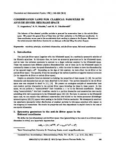
p/2k 0, 0 1, then this function φ cannot be the solution u( · , t) of (C) for any positive time t. It is perhaps simpler to construct a function φ in A that is not of bounded variation. For x between 0 and 1, define 0 for 2−N ≤ x < 1.5 · 2−N , N > 0, φ(x) = 1 for 1.5 · 2−N ≤ x < 2−N +1 , N > 0, with φ(x) = 0 for other values of x. (See Fig. 2.) It is clear that φ(x) can be approximated exactly by a piecewise constant function ψ with 2N knots for 2−N < x < 1. By setting ψ(x) = 0 for x greater than 0 and less than 2−N , one obtains a global error in L1 (R) of less than 2−N with O(N ) knots. In other words, this φ can be approximated exponentially well by piecewise constant functions, and hence is in A for any values of α and q, yet φ is not of bounded variation. Thus, the class A says little about the size of the jumps by themselves, but more about the combination of the size and distribution of the jumps in the functions. The example of a function of bounded variation but not in A had its jumps distributed uniformly in the interval [0, 1], thereby inhibiting good approximation by piecewise linear functions. In contrast, the example of a function in A but not of bounded variation had its jumps concentrated in a very small region. One may conclude intuitively that solutions of (C) that satisfy the hypotheses of Theorem 4.2 may be rough, but they are rough only in very small regions. This intuition is quantified in the atomic decomposition formula given in [7] for functions in Besov spaces. 6. Lack of smoothing. There is, in general, no smoothing in the spaces 1 Aα q (L (It )) for solutions of (C) as t progresses, even if the flux f is uniformly convex. This follows because of the partial reversibility of (C), as described below. Define initial data u0 as follows: Let u0 (x) be zero for x less than 0 and greater than R, and constant between 1 and R, where R is a large parameter to be chosen

9


1 Fig. 2. A function in Aα q (L ([0, 1])) for all α > 1 but not in BV([0, 1]).

later. Between 0 and 1 define u0 (x) by X u0 (x) =

p/2k 0, 0 1.

β 1 1 Then it can be shown that u0 is in any space Aα q (L ([0, 1])) containing A1/r (L ([0, 1])). α 1 Therefore, u( · , t) ∈ Aq (L ([0, R])) for the same values of α and q. Consider the solution u( · , t) of (C) for t between 0 and T for some T when f (u) = u2 . The increasing part of u0 between 0 and 1 spreads out into a series of expansion waves, and there is a shock emanating from the point (R, 0) in (x, t) space. For a fixed T , if R is big enough then these waves will not interact. Consider now the solution of vt + g(v)x = 0, x ∈ R, t > 0,

v(x, 0) = u(x, T ),

x ∈ R,

with g(u) = −u2 . It is easily seen that v(x, T ) = u0 (x) for x between 0 and 1, while the rest of v(x, T ) consists of constant states and a linear function representing a rarefaction wave. It follows that v(x, 0) = u(x, T ) cannot have more smoothness than u0 in the sense of these approximation spaces. It is interesting to note that u( · , t) is piecewise C ∞ for all positive t and is in the Sobolev space W 1,∞ ([0, R]), yet it is not in the spaces Aα q ([0, R]) if α is large enough. 7. Hamilton-Jacobi equations. A special Hamilton-Jacobi equation in one space dimension is given by (H-J)

wt + f (wx ) = 0, w(x, 0) = w0 (x),

x ∈ R,

t > 0,

x ∈ R.

Problems of existence and uniqueness of solutions of (H-J) were solved in papers by M.

10

bradley j. lucier

G. Crandall and P. L. Lions [3], [4], in which they showed that the notion of “viscosity solution” of (H-J) led to well-posedness. Certain “structural” regularity results are known for solutions of (H-J); see, for example, [14]. The problem (C) can be derived formally from (H-J) by setting u = wx and differentiating (H-J) with respect to x. This association is more than formal, however, because Crandall and Lions showed that the viscosity solution of (H-J) is the limit as ǫ tends to zero of the solution of (H-J) with the right-hand side replaced by ǫwxx (hence the name “viscosity solution”). The entropy solution of (C) is also the limit as ǫ tends to zero of the equation with the right-hand side replaced with ǫuxx (see, e.g., [15]), so if w0′ is in L1 , then the formal calculations are in fact valid. Thus one can immediately derive the following theorem from the results in §4. Theorem 7.1. Let w0 have support in [0, 1], and assume that there is an α ∈ 1 (0, 2) and a q ∈ (0, ∞] such that w0′ ∈ BV(R) ∩ Aα q (L ([0, 1])). Assume also that f ′′ ≥ 0, f (0) = 0, and that f ′ and f ′′′ are bounded on Ω (see the comment following Lemma 4.1). Then w( · , t) has support in It = [inf ξ∈Ω f ′ (ξ)t, 1 + supξ∈Ω f ′ (ξ)t] and 1 ′ wx ( · , t) ∈ BV(R) ∩ Aα q (L (It )). In particular, when q = 1/(α + 1) and w0 ∈ BV(R) ∩ α q α q Bq (L (I)), then wx ( · , t) ∈ BV(R) ∩ Bq (L (It )). Acknowledgments. This paper was written after extensive conversations with R. DeVore and V. Popov, and I am deeply indebted to them for their assistance.

REFERENCES [1] R. A. Adams, Sobolev Spaces, Academic Press, New York, 1975. [2] C. de Boor, A Practical Guide to Splines, Springer, New York, 1978. [3] M. G. Crandall and P. L. Lions, Two approximations of solutions of Hamilton-Jacobi equations, Math. Comp., 43 (1984), pp. 1–19. , Viscosity solutions of Hamilton-Jacobi equations, Trans. Amer. Math. Soc., 277 (1983), [4] pp. 1–42. [5] C. M. Dafermos, Generalized characteristics and the structure of solutions of hyperbolic conservation laws, Indiana Univ. Math. J., 26 (1977), pp. 1097–1119. [6] , Regularity and large time behaviour of solutions of a conservation law without convexity, Proc. Roy. Soc. Edinburgh, 99A (1985), pp. 201–239. [7] R. A. DeVore and V. A. Popov, Interpolation of Besov spaces, Trans. Amer. Math. Soc., 305 (1988), pp. 397–414. , Interpolation spaces and non-linear approximation, in Proceedings of the Conference [8] on Interpolation of Operators and Allied Topics in Analysis, Lund, 1986, to appear. [9] R. J. DiPerna, Singularities and oscillations in solutions to conservation laws, Physica, 12D (1984), pp. 363–368. [10] , Singularities of solutions of nonlinear hyperbolic systems of conservation laws, Arch. Rat. Mech. Anal., 60 (1976), pp. 75–100. [11] H. Federer, Geometric Measure Theory, Springer, New York, 1969. [12] J. Glimm, Solutions in the large for nonlinear hyperbolic systems of hyperbolic conservation laws, Comm. Pure Appl. Math., 18 (1965), pp. 697-715. [13] J. Guckenheimer, Solving a single conservation law, in Lecture Notes in Mathematics, 468, Springer-Verlag, Berlin, 1975, pp. 108–134. [14] R. Jensen and P. E. Souganidis, A regularity result for viscosity solutions of Hamilton-Jacobi equations in one space dimension, IMA Preprint Series, 238 (1986). [15] S. N. Kruˇ zkov, First order quasilinear equations in several independent variables, Math. USSR Sbornik, 10 (1970), pp. 217–243. [16] T. P. Liu, Admissible solutions of hyperbolic conservation laws, Mem. Amer. Math. Soc., 240 (1981).


11

[17] B. J. Lucier, A moving mesh numerical method for hyperbolic conservation laws, Math. Comp., 46 (1986), pp. 59–69. [18] O. A. Oleinik, Discontinuous solutions of non-linear differential equations, Usp. Mat. Nauk (N.S.), 12 (1957), pp. 3–73, English translation, Amer. Math. Soc. Transl., Ser. 2, 26, pp. 95–172.. [19] P. Petrushev, Direct and converse theorems for best spline approximation with free knots and Besov spaces, C. R. Acad. Bulgare Sci., 39 (1986), pp. 25–28. , Direct and converse theorems for spline and rational approximation and Besov spaces, [20] in Proceedings of the Conference on Interpolation of Operators and Allied Topics in Analysis, Lund, 1986, to appear. [21] D. G. Schaeffer, A regularity theorem for conservation laws, Adv. in Math., 11 (1973), pp. 368–386. [22] A. I. Vol’pert, The spaces BV and quasilinear equations, Math. USSR Sbornik, 2 (1967), pp. 225–267.