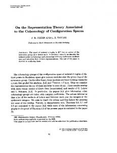
and finite on bounded sets) point process [2]–[5] in R d,d = 1, 2. ... Unique. −2. Fig. 1. Example of an optimal mapping for one dimensional process and. R = 2.
Regularization Energy in Sensor Networks Radha Krishna Ganti and Martin Haenggi Department of Electrical Engineering University of Notre Dame Notre Dame, Indiana, USA-46556 Email: {rganti,mhaenggi}@nd.edu
Interval under consideration
Abstract— Regularization energy is defined as the energy required to move the points of a homogeneous point process in a bounded set to unique points of a lattice. The optimal mapping required for this movement is derived for one dimensional processes, and bounds are derived for the Poisson point process in one and two dimensions. In addition regularization energy is evaluated for well known point processes in one dimension by simulation.
I. I NTRODUCTION In sensor networks, the locations of the sensor nodes are generally modeled as a point process on a plane or on a line. Usually the sensors are not placed in a perfect grid (lattice) due to physical constraints. Sensor networks with randomly placed nodes suffer from severe disadvantages in terms of connectivity, coverage, and efficiency of communication compared with networks with a regular topology. It is of interest to understand the properties of the minimum energy required to move the sensor nodes to unique points of the grid. Another question that arises is how regularly [1] the points of the underlying process are arranged. Thus this regularization energy is also useful to assess the regularity of a point process. II. R EGULARIZATION E NERGY Let φ represent a finite homogeneous (stationary, isotropic and finite on bounded sets) point process [2]–[5] in Rd , d = 1, 2. Regularization energy on a ball B(0, R) is defined as follows. If the energy required to move a unit distance is 1, how much energy is required by the points in the ball to move into a regular grid? Consider a homogeneous point process of intensity 1 on the plane or on a line. Drop an equilateral triangular (simplex in the dimension of space under consideration) mesh M (regularizing mesh) of intensity 1 on the plane. Then the regularization energy is the average minimum energy required to move all the points of the point process inside a ball of radius R centered around origin to distinct lattice points. Defining it mathematically X E(R, M) = E{min kx − f (x)k} (1) f ∈F
x∈φ∩B(0,R)
where F = {f : φ ∩ B → M, and f is one to one } and k.k denotes the distance metric on Rd . Figure 1 illustrates an optimal mapping for a instance of a one dimensional point process. Observe that the points can be mapped to lattice points outside the ball. For R < ∞, E(R, M) < ∞ since
−2
−1
0
1
Unique Mapping
2
Lattice Point Point Process Fig. 1. R=2
Example of an optimal mapping for one dimensional process and
the underlying point process is finite. E(R, M) is a difficult quantity to calculate because the optimal mapping is nontrivial for many point process. This problem is relatively easy to solve for a one dimensional point process, as the optimal mapping can be converted to a tractable optimization problem. III. O PTIMAL MAPPING FOR ONE DIMENSIONAL PROCESSES
For the one dimensional process, the lattice is an equally spaced grid with distance between the lattice points being 1 and B(0, R) is replaced with an interval [−R, R]. The regularization energy is denoted by E(R, δ), where δ denotes the fact that there is a lattice point at δ. Lemma 3.1: Let a1 < a2 < . . . < an be the points of φ ∩ B(0, R) , then for an optimal mapping f , f (ai ) < f (aj ) if i < j. P Proof: Let i < j and f (ai ) > f (aj ) and define S(f ) = |ai − f (ai )|. Interchanging f (ai ) with f (aj ) will give an equal or a smaller value of S(f ). If the order f (a1 ) < f (a2 ) < . . . < f (an ) is not maintained, one can form a new mapping f 0 by a finite number of interchanges of the mapping f such that S(f 0 ) < S(f ). Hence f is not an optimal mapping. Lemma 3.2: Let a, b ∈ φ , a < b and also a, b be neighbors, then for the optimal mapping f , f (b) − f (a) ≤ db − ae. Proof: Let f (b) = f (a) + db − ae + k where k ≥ 0. Case 1: Let f (a) < a, f (b) < b . |a − f (a)| + |b − f (b)| =
a + b − 2f (b) + db − ae + k
By lemma 3.1 there are no points mapped between f (a) and f (b) and hence the minimum value is attained when k = 0.
Case 2: Let f (a) < a, b < f (b) |a − f (a)| + |b − f (b)|
= =
4.5
a − f (a) + f (a) + db − ae + k − b db − ae − (b − a) + k
Poisson Lattice + U(0,1) Beta Process 0.6 Beta Process 0.2 Uniform Matern h=0.45 Matern h=0.2
4 3.5
|a − f (a)| + |b − f (b)| =
j=1
2.5 2 1.5
2f (a) + db − ae − (b + a) + k
The minimum is attained when k = 0. By the above two lemmas, the optimal mapping in one dimension, for the calculation of E(R, δ) can be formulated as the following optimization problem. Divide the process φ ∩ B(0, R) into clusters as follows. Start from the leftmost point and add a point of the process to the same cluster as that of its left nearest neighbor if the distance between the point and its left nearest neighbor is less than 1. Denote by ai the number of points in cluster i, and by γi the ceiling of the distance between the rightmost point of cluster ai and leftmost point of cluster ai+1 , i.e γi = min{d(x − y)e, x ∈ ai+1 , y ∈ ai }. Let x1 < x2 < . . . < xN denote the points of the process φ ∩ B(0, R) and m denote the number of clusters. Let x1 be mapped to the M th lattice point. If xi belongs to cluster ak and is mapped to M 0 , then xi+1 is mapped to M 0 + 1 if it belongs to the same cluster, and is mapped to M 0 + κk if it belongs to the next cluster, where the optimal values of M and κk are determined by the following theorem. Theorem 3.3: The optimal values of M, κi for i = 1 . . . m− 1 ,where |M | ≤ N, 0 ≤ κi ≤ γi are the values that minimize ¾ ak m ½X k−1 X X |M + β(k, j) + κp − xβ(k,j) | (2) k=1
E(R,0)
3
The minimum value is attained when k = 0. Case 3: Let a < f (a) , f (b) < b Then f (b) − f (a) < b − a < db − ae Case 4: Let a < f (a), b < f (b)
p=1
Pk−1 where β(k, j) = p=1 ap + j Proof: Follows from Lemma 3.1 and Lemma 3.2. Since m ≤ bRc, the maximum number of searches required to find the optimum is much less than 2N bRcbRc . Figure 2 gives E(R, 0) for different point processes of intensity 1. From Figure 2, one can observe that E(R, 0) of the Poisson point process (PPP) is a nonlinear and increasing function of R . Also one can observe that the process with larger minimum distance have a lower regulaization energy than processes with lower minimum distance.The process obtained by shifting the lattice uniformly has the lowest E(R, 0). The disturbed lattice process has points which are exactly unit distance from each other (variance of nearest neighbor distance (NND) is zero), which implies that the process is very regular.. This shows that regularization energy can be used as a metric of regularity. Lemma 3.4: E(R, 0) is a increasing and continuous function of R Proof: Let δ > 0. Then E(R, 0) ≤ E(R + δ, 0) − ∗ ∗ ∗ ER+δ [R, R+δ]−ER+δ [−(R+δ), −R] , Where ER+δ [R, R+
1 0.5 0 0.5
1
1.5
2
2.5
3
R
E(R, 0) for processes with λ = 1
Fig. 2.
δ] is the average energy required to map the points in the set [R, R+δ] in the optimal mappings of E(R+δ, 0). This implies E(R, 0) is an increasing function. Since E(φ(δ)) = δ → 0 as ∗ δ → 0, we observe that ER+δ [R, R + δ] → 0 and hence E(R, 0) is a continuous function of R. Lemma 3.5: For any homogeneous point process φ of intensity 1, R/2 bRc/2 + (R − bRc)2 E(R, 0) ≥ dRe/2 − (dRe − R)2
, [R] = 0 , 0 < [R] ≤ 0.5 , [R] > 0.5
where [R] denotes the fractional part of R. This bound is achieved by a homoginized lattice i.e β(1) (Appendix I). Proof: Let V (i) denote the Voronoi region of the ith lattice point with regard to the lattice points. Case 1 : Let [R] ≥ 0.5. Since each point of the process has to move to some lattice point, h E(R, 0)
i min{|x − dxe|, |x − bxc|}
X
≥ E
x∈φ∩[−R, R]
hP i . Let I = E x∈φ∩[−R, R] min{|x − dxe|, |x − bxc|} . Since in the above procedure, the points which get mapped to i are the points of the process which belong to the Voronoi region V (i) h I
=
E
X
X
i |x − i|
i=b−Rc,...,dRe x∈φ∩V (i)∩[−R, R]
=
X
i=b−Rc,...,dRe
h
E
X
x∈φ∩V (i)∩[−R, R]
i |x − i|
Using Campbell’s theorem [2] and using the homogeneity of φ Z d−Re−1/2 (d) I = |x − b−Rc|dx +
Z
X
−1 2
i=d−Re,...,bRc
Z
=
2(2bRc + 1)
1 2
1 2
Z
=
3
|x − dRe|dx bRc+1/2
(dRe − x)dx bRc+1/2
dRe − (dRe − R)2 2
Case 2 : Let 0 < [R] ≤ 0.5. By similar procedure we get, E(R, 0) ≥ Case 3 : Let [R] = 0. By similar procedure we get, E(R, 0) ≥
=
2 1.5 1 0.5
bRc 2
0 0.5
+ (R − bRc)2 .
R 2.
For a homoginized lattice i.e β(1), let the uniform noise in [0, 1] be denoted by U Case 1: [R] = 0. E(R, 0) =
2.5
R
xdx + 2
0
3.5
R
|x|dx + Z
Poisson, E(R,0) Lattice + U(0,1) Uniform Matern h=0.45 Poisson, E(R,0.2) Uniform E(R,0.2) Matern, h=0.45, E(R,0.2) Lattice +U(0,1), E(R,0.2)
4
E(R,0)
−R
4.5
P (U ≤ 0.5)E(U |U < 0.5)2R +P (U > 0.5)E(U |U > 0.5)2R 0.5[2R/4 + 2R/4] = R/2
1
1.5
2
2.5
3
R
Fig. 3.
E(R, M) with lattice at zero and a shifted version.
|x − y| > δ. Let R ∈ Z+ and choose n > 0 such that it is the smallest integer such that 1/n ≤ δ. Then h E(R, 0) ≤ µ0
min
−N ≤x1 ≤N
N X
i |x1 + k(1 − µ0 ) − (1 − 0.5µ0 )|
k=1
(4) where µ0 = 1/n and N = 2Rn. Proof: Since R is an integer and E(R, 0) SNφ+1is homogeneous E(R, 0) = E(R, R). Let B(R, R) = k=1 ξk where ξk = = P (U ≤ [R])(2bRc + 1)[R]/2 [(k − 1)/n, k/n) for k ≤ N and ξN +1 = {2R}. + P ([R] < U ≤ 0.5)(2bRc)((0.5 − [R])/2 + [R]) Define F0 = {f ; f : B(R, R) → Z, f is increasing, f is + P (0.5 < U ≤ 1 − [R])(2bRc)((1 − [R] − 0.5)/2 + [R]) constant on ξk , f (ξk ) 6= f (ξj ) for i 6= j and bounded}. Observe that f ∈ F0 are simple functions [6]. Define X + = + P (U ≥ 1 − [R])(2bRc + 1)[R]/2 {x : f (x) ≥ x}, X − = {x : f (x) < x}. Also X + ∩ X − = ∅ = bRc/2 + (R − bRc)2 and X + ∪ X − = B(R, R). Let µ(.) denote the standard Lebesgue measure [6]. Case 3: [R] ≥ 0.5. Similarly we get The functions of F0 restricted to φ belong to F and hence E(R, 0) = dRe/2 + (dRe − R)2 h i X E(R, 0) = E inf 0 kx − f (x)k f ∈F x∈φ∩B(R,R) Is regularization energy invariant with regard to the position of lattice, i.e. is E(R, 0) = E(R, δ)? One can observe that E(R, 0) = E(R, k) where k is an integer. Also E(R, δ) = E(R, 1 − δ), since the underlying point process looks the same Since F does not depend on φ, the expectation can be moved (invariant) from −R and R and relative to the lattice. So it inside. Hence suffices to check for 0 ≤ δ ≤ 0.5. It is not true in general that h i X E(R, 0) = E(R, δ). For example in the case of lattice disturbed E(R, 0) ≤ inf 0 E kx − f (x)k f ∈F by uniform noise, when [R] = 0, E(R, δ) = E(R, 0) = R/2. x∈φ∩B(R,R) But if 0 < [R] < 0.5, δ < [R] and δ + [R] < 0.5, then hP i . E(R, δ) = bRc/2 + (R − bRc)2 + δ 2 (3) Let I(f ) = E kx − f (x)k . Then x∈φ∩B(R,R) Case 2: 0 < [R] < 0.5.
So in general, E(R, δ) 6= E(R, 0). Theorem 3.6: Let φ be a one-dimensional homogeneous point process with intensity λ = 1, such that ∀x, y ∈ φ ⇒
h I(f )
= E
X x∈φ∩X +
(f (x) − x) −
X x∈φ∩X −
i (f (x) − x)
Since X + , X − are measurable bounded sets, Campbell’s theorem [2] can be applied Z hZ i I(f ) = (f (x) − x)dx − (f (x) − x)dx X+ Z ZX − Z hZ i = ( f− f) − ( x− x) X+
X−
X+
I(f ) = +
Z Zk=1 xdx − [
µ0
•
i xdx] X+
By construction of ξk and definition of f , µ(ξk ∩ X + ), µ(ξk ∩ X − ) can be only µ(ξk ) or 0. Let K + = {k : f (ck ) > ck }, K − = {k : f (ck ) < ck }. Then i h X X (f (ck ) − ck ) I(f ) = µ0 (f (ck ) − ck ) − k∈K + N X
B
x∈φ
f (ck )[µ(ξk ∩ X + ) − µ(ξk ∩ X − )]
X−
=
•
X−
Let ck be the mid point of ξk , i.e., ck = (k − 0.5)µ0 . Since f is a simple function, N hX
•
0 0 0 one √ can use exp(−λ VC ) = (1 − λ VC ), so we get λ ≈ ²/VC , where p volume p VC is the √ of the cell. Choose α = λ/λ0 = λVC / ² TheP energy expended in the above process is E( x∈φ kαx − xk). Using Campbell’s theorem [2] Z X E( kαx − xk) = λ|α − 1| kxkdx (6)
The new process formed by expansion of the old process is also a Poisson point process [7, pg 18]. Once there is only one or zero point in each Voronoi region of the reference lattice, the optimal solution would be to move to the center of the Voronoi cell. The energy for the point in one Voronoi cell to move to the center is Z Ev = kxkdx (7) C
•
k∈K − •
|f (ck ) − ck |
k=1
Hence E(R, 0) ≤ inf 0 I(f )
The number of Voronoi cells in B is approximately VB /VC and the probability for each Voronoi cell to contain one point is λ0 VC exp(−λ0 VC ) The total energy expended is Z Er (B) / λ|α − 1| kxkdx B Z +(VB /VC )λ0 VC exp(−λ0 VC ) kxkdx C
f ∈F
(a)
= µ0
h min
−N ≤x1 ≤N
N X
i |x1 + k(1 − µ0 ) − (1 − 0.5µ0 )|
•
(5)
k=1
(a) follows from lemma 3.2 and the fact that f is increasing ( hence for the optimal f , f (ck+1 ) = f (ck ) + 1). h PN Also µ0 min−N ≤x1 ≤N k=1 |x1 + k(1 − µ0 ) − (1 − i 0.5µ0 )| ≈ (d1/δe − 1)R2 for δ < 1. This can be verified by simulation.
A lower bound can be obtained as follows. • •
IV. E(R, M) BOUNDS FOR P OISSON P OINT P ROCESS (PPP) IN TWO DIMENSIONS
A heuristic upper bound can be obtained on E(R, M) for PPP of intensity λ. Let the volume of the Voronoi region (cell) of a lattice point in the mesh M be VR . The idea is as follows. If only one point of the process φ exists in a Voronoi cell C of the regularizing lattice, the optimal mapping would be to move the point to the center (lattice point ) of the Voronoi cell. • Let ² be very small number. • Expand points of φ by a factor α forming a new process φ0 . Chose α such that with high probability, only one or zero points appear in a Voronoi cell of the original reference lattice. Let λ0 be the new intensity. i.e., Choose α such that, P (φ0 (C) = 0) + P (φ0 (C) = 1) = 1 − ², i.e exp(−λ0 VC )(1 + λ0 VC ) = 1 − ² . If λ0 is very small,
When B = B(0, R), the normalized Er (B) is s ´ E(R, M) 2 ³ λVC √ −1 R / λ 2 πR 3 ² √ √ Z ² exp(− ²) + kxkdx VC C
•
•
Consider the Voronoi cells C of the regularizing lattice. Move the points of φ in a Voronoi cell to the center of the cell. This certainly lower-bounds E(R, M) because, each point x ∈ φ is closer to the center of the Voronoi cell to which it belongs rather than to any lattice point. Movement to any other lattice point would require more energy. For a PPP of intensity λ, the energy required for this procedure is given by Z VB λ kxkdx (8) E(R, M) ≥ VC C
An interesting but suboptimal mapping is as follows • • • •
Find the Voronoi regions of the reference lattice. In each Voronoi cell map the center of the cell to the nearest x ∈ φ. Remove the mapped points of the lattice and φ. Continue this procedure with the remaining lattice points and the remaining points of the process φ.
V. C ONCLUSION In this paper the minimum average energy (regularization energy) required to move the points of a point process to unique lattice points is defined. The mapping that attains the minimum energy is proposed for one dimensional processes. The regularization energy has been evaluated for one dimensional process by simulation. It is observed from simulations that regular processes have lower regularization energy and regularization energy is invariant with respect to lattice position for some one dimensional processes. Lower and upper bounds have been proposed for one dimensional processes. Hueristic bounds on regularization energy for two dimensional PPP have been presented. A PPENDIX I B ETA PROCESS Beta process is a homogeneous process of intensity 1 and is parameterized by 0 < β < 2.
B(β) =
h[
i {2k, β + 2k} + U (0, max{β, 2 − β})
k∈Z
where U (a, b) represents a uniform random variable between a and b R EFERENCES [1] R. K. Ganti and M. Haenggi, “Regularity in Sensor Networks”, International Zurich Seminar on Communications, Feb. 2006. [2] Dietrich Stoyan, Wilfrid, S. Kendall, and Joseph Mecke, Stochastic Geometry and its Applications, Wiley, New York, 1995. [3] D. J. Daley and D. Vere-Jones, An Introduction to the Theory of Point Processes, Springer, New York, second edition, 1998. [4] Olav Kallenberg, Random Measures, Akademie-Verlag, Berlin, 1983. [5] D. R. Cox and Valerie Isham, Point Processes, Chapman and Hall, London and New York, 1980. [6] Gerald B. Folland, Real Analysis, Modern Techniques and Their Applications, Wiley, 1999. [7] J.F.C. Kingman, Poisson Process, Oxford University Press.


![columbus - Notre Dame Campus Tour - University of Notre Dame [PDF]](https://m.moam.info/img/260x300/columbus-notre-dame-campus-tour-university-of-notr_6479c497098a9ef8668b4658.jpg)