translation). More details about the nomenclature and the wavelet packets can be found in Galiana-Merino et al. (2003). For any wavelet packet decomposition ...
Bulletin of the Seismological Society of America, Vol. 94, No. 4, pp. 1467–1475, August 2004
Regularized Deconvolution of Local Short-Period Seismograms in the Wavelet Packet Domain by J. J. Galiana-Merino, J. Rosa-Herranz, J. Giner, S. Molina, and F. Botella
Abstract Short-period seismographs of the vertical component have a frequency response similar to a bandpass filter with a low cutoff frequency around 1 Hz. This instrument’s response distorts in some way the interesting signal that arrives at the sensor. In this case, the aim of the deconvolution is at recover the signal as it arrives at the sensor, since this signal can be very important to the study of source mechanisms, for instance. In this article we present a new method of regularized inversion based on the wavelet packet transform. This method achieves the deconvolution of the instrument response through the time–frequency information contained in the wavelet packet transform of the signals. Although the instrument response is known (Ja´uregui, 1997), the noise and other artifacts in the signal make deconvolution a nontrivial process. As an evaluation method, we first apply it to synthetic signals we generated. In this way, the shape of the whole output signal and the onset time of the first pulse can be compared to the ideal signal. The method is also applied to real signals, specifically to local short-period seismograms registered at the seismic network of the University of Alicante in southeastern Spain. In both cases, the results are compared with the water-level correction method currently used. The comparison shows how the proposed method works better, as it provides, in contrast to the current method, the shape and the onset time of the ideal signal. Introduction Deconvolution is a very common subject in image and signal processing, with applications ranging from the restoration of satellite images to the equalization of communication channels; it also has applications in seismology. In this article, the deconvolution process is focused on a real problem that affects most short-period seismograms and particularly the ones recorded by the local seismic network of the University of Alicante (LSNUA). These seismograms are distorted by the instrument response of the acquisition and recording system. If we want to obtain the real ground movement at the sensor position, we will need to remove the effects introduced by the set of instruments. Basically, we must deconvolve the impulse responses of the equipment from the real seismograms. Once we have the signal as it arrives at the sensor, without the distortion of the instrument response, we may use it to study the characteristics of the source and the propagation. Moreover, the deconvolved signal may be convolved with the instrument responses of other systems, which allows us to carry out comparisons of amplitude and arrival times between different classes of sensors. The deconvolved signal may be also convolved with the instrument response of a Wood–Anderson
seismograph to measure the local magnitude ML of the earthquake. Theoretically, if the impulse response of the instruments is known, the deconvolution should be an easy process. However, it is more difficult because real seismograms are contaminated by noise. In fact, this deconvolved signal is seriously distorted with a high level of noise. That is because the part of the signal spectrum that is out of the system passband is amplified. Furthermore, the steeper the transition band is, the greater this amplification. The problem is that the part of the signal spectrum that is amplified is generally noise. With the aim of avoiding the amplification of the noise, the influence of the instrument response may be corrected only within a specific frequency band. This frequency band is not fixed and depends on the level of noise as much as the slope of the frequency response of the system. One commonly applied method to minimize this problem is the waterlevel correction (WLC) method, which bounds the minimum amplitude of the frequency response of the system. In this article, we propose an alternative method that is based on the discrete wavelet packet transform (DWPT). One
1467
1468
J. J. Galiana-Merino, J. Rosa-Herranz, J. Giner, S. Molina, and F. Botella
advantage of the signal decomposition by wavelet packets is that it allows selection of the time–frequency decomposition that best suits the studied signal. In this way, we can detect the frequency bands of the signal that are seriously contaminated by noise (with a low signal-to-noise ratio [SNR]) and we can modify properly the frequency response of the system in order to avoid noise amplification during the deconvolution process. In the following sections, we present a theoretical introduction to the wavelets and the deconvolution problem and explain the proposed method. We also present experimental results that are compared with the current method of deconvolution that is used at the University of Alicante.
The Wavelet Packet Transform The analysis in time or frequency separately is not the most appropriate approach for nonstationay signals. An analysis carried out in both domains is more desirable (Steeghs, 1997). In this article we use the DWPT, which allows us to decompose the time–frequency plane in such a way that it efficiently matches the signal. Using this approach, we can obtain a high time (or frequency) resolution in the frequency bands where it is more necessary. The DWPT is implemented using a subband coding scheme, three stages of which are illustrated in Figure 1. The original signal is represented by k0,0(n), and the operators H and G represent linear convolution plus downsampling by a factor of 2 (removal of every other sample). In terms of the discrete wavelet transform, H is known as the wavelet filter and is derived from the corresponding mother wavelet and G is the scaling filter. We have adopted the nomenclature of Wickerhauser (1994), where j is the scale index, r is an index associated with the frequency bands, and n is an index of position (or translation). More details about the nomenclature and the wavelet packets can be found in Galiana-Merino et al. (2003).
For any wavelet packet decomposition of J scales, we have many different signals, kj,r(n), whose appropriate union can provide an equivalent representation of the original signal, k0,0(n). For instance, in Figure 1 we can obtain equivalent representations of k0,0(n) through the following sets of signals or nodes: {k1,1(n), k2,1(n), k3,0(n), k3,1(n)}, {k2,0(n), k2,2(n), k2,3(n), k3,2(n), k3,3(n)}, and so forth. The node selection process is achieved through an entropy function that is applied on every node of the decomposition (Wickerhauser, 1994). The only requirement is that the bandwidth of the original signal must be covered by the chosen set of signals, without overlapping, in such a way that each signal, kj,r(n), will be associated with a frequency band.
Deconvolution of Signals Contaminated by Noise A digital seismic signal x(n) can be represented through the following expression: x(n) ⳱ h(n) * [s(n) Ⳮ z1(n)] Ⳮ z2(n),
(1)
where h(n) is the impulse response of the system used (sensor, amplifiers, filters, etc.), s(n) represents the groundmotion signal, z1(n) is natural noise, and z2(n) is noise from the different elements of the acquisition system. Combining the different noise terms, a simpler expression is obtained from equation (1): x(n) ⳱ h(n) * s(n) Ⳮ z(n).
(2)
The aim is to get the seismic signal s(n) as it arrives at the sensor, removing as much as possible the noise and the spurious effects introduced by the equipment. For this purpose, a combination of filtering and deconvolution must be performed. In the frequency domain, equation (2) can be expressed as X( f ) ⳱ H( f ) • S( f ) Ⳮ Z(f ).
(3)
Figure 1. Tree structure of the wavelet packet analysis. H and G are the low and high digital filters, respectively, and kj,r(n) are the different signals associated with every node of the decomposition. In this nomenclature, each node is characterized by a pair of numbers (j,r), where j is the scale index and r is the index associated with the frequency or the position within a scale.
Regularized Deconvolution of Local Short-Period Seismograms in the Wavelet Packet Domain
If the instrument response is known, as usually occurs, the signal S(f ) can be obtained approximately by S( f ) ⳱
X( f ) Z( f ) ⳮ . H( f ) H( f )
(4)
In the absence of noise, the signal S(f ) could be calculated without any error, supposing that H(f ) ⬆ 0 between 0 and the Nyquist frequency. Nevertheless this is not the real situation. If H(f ) is very small for some sets of frequencies, the signal of interest will be poorly recovered and hidden by a high level of noise as the term Z(f )/H(f ) becomes very large. To carry out the deconvolution process with the minimum noise amplification, there are several alternative methods to the pure inversion in the Fourier domain (equation 4). These methods can be classified in two groups depending on whether they are a pure inversion or a regularized inversion in the Fourier domain. Pure Inversion in the Fourier Domain This kind of method applies the following scheme: 1. Use the frequency response of the system, H(f ), and equation (4) to accomplish the deconvolution. 2. Filter the signal obtained in step 1 to reduce the noise. The simplest way of carrying out the second stage is through a digital bandpass filter. However, this is not enough to eliminate satisfactorily the high noise level following deconvolution. Moreover, the digital filter could add a new distortion on the signal. Another more effective means of reducing noise can be achieved by using a filter based on the wavelet transform. This technique comes from the method of wavelet–vaguellete decomposition proposed by Donoho (1995). However, after a pure inversion in the Fourier domain, the variance of the resulting noise can be as high in the signal as in the wavelet coefficients; thus filtering by wavelet transform can be also inefficient. Regularized Inversion in the Fourier Domain In this case, the frequency response of the signal obtained after deconvolution is modified in such a way that the amplitude of the frequency components related to noise are reduced. The aim of the regularization is to reduce the noise and achieve a better estimation of the expected signal in return for a small distortion on the signal (Tikhonov and Arsenin, 1977). A basic scheme can be expressed by the following two steps: 1. Apply a pure inversion in the Fourier domain to obtain the spectrum of the deconvolved signal, which is contaminated with a high level of noise. 2. Estimate the signal in the Fourier domain. In this stage,
1469
the amplitude of some frequency components is modified through a weighting function. This new approach to the deconvolution problem was first introduced by Tikhonov and Arsenin (1977), and their method is called windowed singular value decomposition. The optimum weights that can be used for carrying out the regularized deconvolution depend on the SNR associated with each frequency component. For stochastic signals contaminated with Gaussian noise, the linear time invariant Wiener deconvolution filter provides an optimal estimate of the signal in the sense of the minimum square error. However, it does not provide a good solution for nonstochastic signals with well-localized characteristics (pulses, discontinuities, etc.) in the time domain (Neelanami, 1999). This method and other similar ones require an estimate of the expected signal, which is achieved through an iterative application of the deconvolution method. Another simpler method of regularized inversion is the WLC used by Scherbaum (1996) on real seismograms. In this approach, the amplitude of the frequency response of the system, H(f ), is assigned some nonzero, constant, lower threshold, whereas the phase remains the same. There is not a general rule to determine the threshold, only that it has to be enough to ensure the stability of the system. This deconvolution method is currently used by the LSNUA. In their algorithm, the threshold is just the amplitude of the spectrum at some frequency below the Nyquist rate. Finally, a standard bandpass filter is applied for reducing the noise. We propose a new, regularized deconvolution method based on wavelet packets (ReDWP). The basic idea consists of modifying the frequency response of the system according to the variance of the noise associated with every node of the wavelet packet decomposition. We also apply a previous and subsequent denoising stage by means of the wavelet packet transform (Galiana-Merino et al., 2003). In our real case, the noise can be characterized for every recorded signal since we use a few seconds before the first signal pulse as a sample of the noise. As a future step, it would be very interesting to use an assumed standard noise and combine the proposed method with a Bayesian approach (e.g., Ulrych et al., 2000).
Regularized Deconvolution based on Wavelet Packets The proposed method can be decomposed into three steps. The first and the last are denoising processes in the wavelet packet domain. The second step is the regularized deconvolution of the instrument, which we develop herein. Denoising In this step, we have adapted the method proposed by Donoho and Johnstone (1994) to a more realistic situation
1470
J. J. Galiana-Merino, J. Rosa-Herranz, J. Giner, S. Molina, and F. Botella
where the noise, z(n), is not necessarily white noise, as is usually assumed. We can accomplish the denoising process through the following steps: 1. Extract a sample of noise, z⬘(n), from several seconds before the first pulse of the signal x(n). 2. Apply the DWPT to x(n) and z⬘(n) in order to obtain a complete tree structure decomposition. After that, determine the subset of nodes that best fits the signal x(n) for a chosen entropy function and select this subset of nodes for both x(n) and z⬘(n). In this way, both signals are composed of two sets of coefficients kj,r(k)|x and kj,r(k)|z⬘. 3. In the case of x(n), the coefficients are also contaminated by noise. Thus they can be expressed as a composition of coefficients related to signal and coefficients related to noise: kj,r(n)|x ⳱ kj,r(n)|h*s Ⳮ kj,r(n)|z.
(7)
If a good basis (subset of nodes) and a good mother wavelet are chosen, the coefficients kj,r(k)|h*s will be reduced to only a few large coefficients and the rest will be negligible. In this way, we can apply thresholding methods over the wavelet packet coefficients and reduce the noise considerabily. In our case, we have used a soft thresholding (Donoho, 1995) with a node-dependent threshold (Galiana-Merino et al., 2003). 4. Finally, apply the inverse wavelet packet transform to obtain the signal xˆ(n). Deconvolution After the first stage, we obtain a signal xˆ(n) where the noise is reduced considerably. Nevertheless, a deconvolution based on a pure inversion in the Fourier domain produces an expression as equation (8) and then it presents the same problems as before, unless Z⬘(f ) is zero: ˆ ˆ f ) ⳱ X( f ) ⳮ Z⬘( f ) . S( H( f ) H( f )
(8)
We propose an algorithm that uses a regularized inversion in the Fourier domain and an estimate of the modified instrument response in the wavelet packet domain. As the wavelet packet bases are well located, as much in time as in frequency, they provide an appropriate tool for processing nonstationary signals with some well-localized time characteristics. The proposed method can be split into several steps: 1. Extract a noise sample, zˆ⬘(n), from the initial seconds of the denoised signal. 2. Apply the DWPT to the signals xˆ(n) and zˆ⬘(n) and obtain two sets of wavelet packet coefficients kj,r(n)|xˆ and kj,r(n)|zˆ⬘. In this way, we obtain a time–frequency decom-
position adapted to the characteristics of the signal, where every node is associated with a different frequency band. 3. Determine the variance of the coefficients associated with every node of the signal and noise. The nodes of the signal decomposition that are seriously contaminated with noise present a variance, rj,r|xˆ, that is very similar to the variance of the noise decomposition, rj,r|zˆ⬘, associated with the same nodes. With this criterion, the nodes of the signal decomposition that are seriously contaminated with noise are determined. 4. According to the information obtained in the previous step, modify the frequency response of the system in this way: ˆ j,r( f ) ⳱ |Hj,r( f )| • e j; if rj,r|xˆ � rj,r|zˆ⬘ then H ˆ j,r( f ) ⳱ |A| • e j, if rj,r|xˆ ⱕ rj,r|zˆ⬘ then H
(9)
where Hj,r(f ) means that the change done over H(f ) only affects the frequency band associated with the node (j,r) and is the phase of Hj,r(f ). |A| is a maximum bound that can be chosen as max{|H(f )|}, and it ensures that the noise is not amplified more than the signal. In both cases, the phase remains the same, thus avoiding a time shift on the signal. In the case of short-period seismograms recorded by the local seismic network, the frequency band is limited. This is also addressed, and then the frequencies out of the passband of the instrument response are modified as discussed earlier. 5. Divide the frequency response of the filtered signal by the modified frequency response of the system. In the frequency bands where the signal can be viewed as noise, the spectrum is attenuated by a factor |A|. For the rest of the nodes, the spectral division is performed with the frequency response of the system associated with these nodes. In this way, we obtain an estimate of the signal in the frequency domain. 6. Finally, apply the inverse Fourier transform to obtain the deconvolved signal in the time domain, sˆ(n). In some cases, the SNR of the obtained signal can be improved following the same denoising process that was explained in the previous section.
Evaluation of the ReDWP Method To test the proposed method, it is first applied to synthetic signals we generated. The source parameters are deduced by applying the Brune (1970, 1971) source function model. Then a local model of three homogeneous layers (Ja´uregui, 1997) is used to generate the complete pure synthetic signal, s(n). The simulation follows a raytracing scheme that includes body and Rayleigh waves. Finally, the signal is convolved with the instrument response, h(n), and mixed with real noise from the region, z(n), which has been amplified in order to obtain the desired SNR. In this way, we
Regularized Deconvolution of Local Short-Period Seismograms in the Wavelet Packet Domain
obtain the desired synthetic signal x(n). Figure 2 shows an example of one of these synthetic signals. In Figure 3, a comparison is made between the spectrum of this synthetic signal and the spectrum of a real seismogram. This figure shows that the frequency components of higher amplitude in the synthetic signal are in a range very similar to that of real seismograms: between 4 and 7 Hz. The proposed method is now applied to the signal x(n), and the output signal sˆ(n) is compared to the original s(n). Apart from the SNR, there are other parameters that would be interesting to analyze. For instance, it is very important that the shape of the signal and, above all, that the shape of the first pulse (generally the P arrival) are not distorted. Obviously, it is also important to avoid any undetermined delay in the signal. This is the reason for choosing the following comparison parameters: energy rate, SNR, autocorrelation coefficient of the whole signal, and autocorrelation coefficient of the first pulse. To apply the proposed deconvolution method, it is necessary to determine first the parameters associated with the DWPT: mother wavelet, entropy function, and maximum level of decomposition. Although some parameters and functions can seem to be better than others, it is difficult to discriminate among them without first examining their effects on the sort of signals under study. We have therefore applied the proposed method to a large set of synthetic signals having similar characteristics to the real seismograms, using different kinds and combinations of mother wavelet, entropy function, and maximum level of decomposition. From this analysis, we have chosen the parameters that provided the best results: Daubechies 10 or 12 as a mother wavelet (Daubechies, 1992), Shannon entropy (Wickerhauser, 1994) or an entropy based on the energy under some threshold (Storm, 1997), and a maximum level of decomposition between 5 and 6. With these choices, we have found that the autocorrelation coefficient of the whole signal is above 0.98 and the autocorrelation coefficient of the first pulse is around 0.94, with an energy variation lower than 5% compared to the expected signal. Moreover, the SNR is above 26 dB in all cases (Galiana-Merino, 2001). The set of mother wavelets that we have used in the test is restricted to those implemented in the Matlab software, since our aim is to evaluate the proposed deconvolution method and not necessarily the mother wavelet that best performs this task. It is likely that our next step should be to improve the parameters that we have used, such as exploring the benefits of adopting a different mother wavelet (e.g., Lilly and Park, 1995). To compare the ReDWP method with the currently used WLC method, we have applied the WLC method to the same signals and have taken the same quantitative measures as above. With the WLC method, the autocorrelation coefficient of the whole signal barely reaches the value of 0.76 and the autocorrelation coefficient of the first pulse does not exceed 0.13 for the best case, when we used a threshold equal the
Figure 2. Synthetic signal, x(n), generated at a distance of 21 km and a depth of 1 km, with an SNR equal to 14 dB. The sample frequency equals 100 Hz.
Figure 3. (a) Spectrum of the synthetic signal of Figure 1. (b) Spectrum of a local short-period seismogram registered by the local seismic network of the University of Alicante (southeast Spain).
1471
1472
J. J. Galiana-Merino, J. Rosa-Herranz, J. Giner, S. Molina, and F. Botella
amplitude of the spectrum at the frequency of 0.65 times the Nyquist frequency. Regarding the SNR, it is around 14 dB, and in several cases it is also worse than in the original signal (Galiana-Merino, 2001). In Table 1 we compare the quantitative results obtained from both methods. In Figure 4, we compare graphically the signals obtained by both methods with the expected signal. In Figure 5, we zoom in on the first pulse of all these signals in order to compare them better. In these graphs we have also marked with an arrow the pick determined by an expert analyst. In this way, we can observe that the signal obtained with the ReDWP method presents a very small distortion around the first pulse. This pulse is clearly identified, and both the polarity and the onset time (6.27 sec) are recovered without any mistake. In the case of the WLC method, the first pulse presents a distorted shape with two peaks of great amplitude and different polarity where there should be only one. Moreover, the processed signal presents a time shift with respect to the expected signal that produces an incorrect onset pick. The onset occurs at 6.20 sec, meaning that the WLC method has advanced the first pulse 0.07 sec with respect to the expected signal.
Application of the ReDWP Method to Real Seismograms In this section, we apply the proposed method to shortperiod seismograms recorded in the province of Alicante (southeast Spain); an example of these is presented in Figure 6a. Using the same approach as in the last section, we apply the ReDWP and WLC methods to these events and compare the results obtained in each case (Fig. 6b,c). The application of ReDWP improves the SNR to 49 dB and obtains a very clear first pulse. In contrast, the WLC method obtains a signal with an SNR of 23 dB, which is worse than the SNR of the original signal. In Figure 7, we zoom in on the first pulse to compare the original signal (distorted by the instrument response and contaminated by noise) with the signals obtained by the application of ReDWP and WLC methods. In this figure the arrows indicate the pick determined by an expert analyst on every signal, although we have already demonstrated in the
Figure 4.
(a) Pure synthetic signal, s(n). (b) Signal deconvolved with the ReDWP method. (c) Signal deconvolved with the WLC method.
Table 1 Evaluation Parameters Associated with the Deconvolution Methods
Deconvolution Method
ReDWP WLC
Energy of the Processed Signal with Respect to the Pure Synthetic Signal (%)
101.8 97.8
Signal-to-Noise Ratio (dB)
Autocorrelation Coefficient between the Processed Signal and the Pure Synthetic Signal
Correlation Coefficient between the First Pulse of the Processed Signal and the First Pulse of the Pure Synthetic Signal
31 16
0.98 0.76
0.92 0.13
ReDWP is with a Daubechies 10 mother wavelet and Shannon entropy and WLC is with a minimum magnitude level fixed at 65% of the Nyquist frequency.
Regularized Deconvolution of Local Short-Period Seismograms in the Wavelet Packet Domain
Figure 5. Zoom of the first pulse of the signals of the Figure 4. (a) Pure synthetic signal, s(n). (b) Signal deconvolved with the ReDWP method. (c) Signal deconvolved with the WLC method. In these graphs the arrows indicate the pick determined by an expert analyst of the local seismic network.
evaluation process that only the ReDWP method corrects the time shift introduced by the instrument response. Now we cannot compare the obtained result with the ideal signal since we are using real signals. Moreover, there are several differences between the first pulse of the recorded signal and the signal obtained after deconvolution by ReDWP. These differences affect not only to the shape of the signal, but also to the onset time. Initially, it seems that ReDWP introduces a time shift to the signal, producing an incorrect onset time. However, we cannot forget that we are comparing the obtained pulse with the pulse of the recorded
1473
Figure 6. (a) Vertical component of a local shortperiod seismogram of a magnitude ML 1.6 earthquake, located at Torrrevieja (37.56� N, 0.37� W) and recordered with an SNR of 25 dB. (b) Signal deconvolved with the ReDWP method. The parameters are Daubechies 12 as the mother wavelet and Shannon entropy as the cost function. As a sample of noise we select the first 4 sec of the signal. (c) Signal deconvolved with the WLC method. The reference frequency is 65% of the Nyquist frequency.
signal, which is affected by the instrument response. In Figure 8 we compare the first pulse of a pure synthetic seismogram before and after convolution with the instrument response of one of the stations. This figure shows very clearly how the recorded pulse (which is convolved with the instrument response) presents a shape quite different from the pulse of the signal that arrives at the sensor (which is not yet convolved). Moreover, the recorded signal presents a time shift of 0.03 sec (three samples) with respect to the signal that shows the ground motion.
1474
J. J. Galiana-Merino, J. Rosa-Herranz, J. Giner, S. Molina, and F. Botella
Figure 8. Figure 7. Zoom of the first pulse of the signals of the Figure 6. (a) Real seismogram. (b) Signal deconvolved with the ReDWP method. (c) Signal deconvolved with the WLC method. In these graphs the arrows indicate the pick determined for every signal by an expert analyst.
Conclusion In any deconvolution process, the regularized inversion in the Fourier domain provides the best results when the analyzed signal is contaminated with noise. However, the deconvolution method used at the LSNUA, the WLC method, does not reduce properly the distortion introduced by the instruments, and it increases the noise level on the resulting signal, as we have shown in both synthetic and real cases. We have proposed a new regularized deconvolution method that is based on the properties of the wavelet packets, because of their time–frequency localization characteristics and the adaptability to different kinds of signals through the
(a) Pure synthetic signal as it arrives at the sensor. (b) Synthetic signal from (a) convolved with the instrument response of the acquisition system.
entropy function. For the analyzed signals, this method provides the correct onset time, distorts the signal very little, and improves considerably the SNR. Moreover, in contrast to the deconvolution filter of Wiener, our method does not require a priori information about the desired signal. The parameters used in the ReDWP method (mother wavelet, entropy function, and maximum level of decomposition) can change depending upon the station and its site properties. Nevertheless, after the test with synthetic signals we conclude that we can maintain a fixed set of parameters with good results. From the evaluation process with synthetic signals, we obtain the following measures of interest: an autocorrelation coefficient between the processed signal and the expected signal over 0.98, an autocorrelation coefficient between the first pulse of the processed signal and the first pulse of the
Regularized Deconvolution of Local Short-Period Seismograms in the Wavelet Packet Domain
desired signal around 0.94, an SNR over 26 dB, and an energy difference between both signals of less than 5%. When we apply the ReDWP method to real seismograms, it provides deconvolved signals with a good SNR that allows us to identify clearly the onset time and the polarity of the first pulse. Finally, we have also shown the effects that the instrument response has on the signal that arrives at the station sensor. One of these effects is a time shift that the instruments introduce to the signal. In the analyzed signals, this effect is also corrected by the ReDWP method.
Acknowledgments We are grateful to the research group of the local seismic network of the University of Alicante (supported by Diputacio´n de Alicante) and especially to Dr. P. Ja´uregui for his help in analyzing and presenting the data. We also acknowledge the financial support of the Spanish Ministry of Science and Technology (MCYT) under Project TIC2002-04451-C02-02 and Instituto Alicantino de Cultura Juan Gil-Albert (Diputacio´n de Alicante): RE.847-M and RE.851-M. We are very thankful to Jeffrey Park for his suggestions on this subject. We also thank Tadeusz Ulrych and an anonymous reviewer for their comments, which helped us to clarify and improve this article. Finally, we would also like to thank the associate editor, Charlotte A. Rowe, for her valuable feedback regarding the content and style of the original manuscript.
References Brune, J. (1970). Tectonic stress and the spectra of seismic shear waves from earthquakes, J. Geophys. Res. 75, no. 26, 4997–5009. Brune, J. (1971). Correction to tectonic stress and the spectra of seismic shear waves from earthquakes, J. Geophys. Res. 76, no. 20, 5002. Daubechies, I. (1992). Ten Lectures on Wavelets, SIAM, Philadelphia. Donoho, D. (1995). Nonlinear solution of linear inverse problems by wavelet-vaguellete decomposition, App. Comput. Harmonic Anal. 2, 101– 126. Donoho, D., and I. M. Johnstone (1994). Ideal spatial adaptation by wavelet shrinkage, Biometrika 81, 425–455. Galiana-Merino, J. J. (2001). Aplicacio´n de la transformada de wavelet a sismogramas locales: filtrado, deconvolucio´n y estimacio´n del a´ngulo azimut (in Spanish), Ph.D. Thesis, Universidad de Alicante, Spain.
1475
Galiana-Merino, J. J., J. Rosa-Herranz, J. Giner, S. Molina, and F. Botella (2003). De-noising of short period seismograms by wavelet packet transform, Bull. Seism. Soc. Am. 93, no. 6, 2554–2562. Ja´uregui, P. (1997). Estudio de la operatividad de redes sı´smicas locales aplicado a la optimizacio´n de los recursos de la Red Sı´smica Local de la Universidad de Alicante (in Spanish), Ph.D. Thesis, Universidad de Alicante, Spain. Lilly, J. M., and J. Park (1995). Multiwavelet spectral and polarization analyses of seismic records, Geophys. J. Int. 122, 1001–1021. Neelamani, R. (1999). Wavelet-based deconvolution for ill-conditioned systems, Ph.D. Thesis, Rice University, Houston, Texas. Scherbaum, F. (1996). Of Poles and Zeros: Fundamentals of Digital Seismology, Kluwer, Hingham, Massachusetts. Steeghs, P. (1997). Local power spectra and seismic interpretation, Ph.D. Thesis, Delft University of Technology, The Netherlands. Storm, H. (1997). Noise reduction of speech signals with wavelets, Ph.D. Thesis, Chalmers University of Technology and Go¨teborg University, Go¨teborg, Sweden. Tikhonov, A. N., and V. Y. Arsenin (1977). Solutions of Ill-Posed problems, V. H. Winston, Washington, D.C. Ulrych, T. J., M. D. Sacchi, and A. D. Woodbury (2000). A Bayes tour of inversion: a tutorial, Geophysics 66, no. 1, 55–69 Wickerhauser, M. V. (1994). Adapted Wavelet Analysis from Theory to Software, A. K. Peters, Wellesley, Massachusetts. Departamento de Fı´sica Ingenierı´a de Sistemas y Teorı´a de la Sen˜al Escuela Polite´cnica Superior Universidad de Alicante Ap. Correos 99, 03080 Alicante, Spain (J.J.G.-M., J.R.-H.) Departamento de Ciencias de la Tierra y del Medio Ambiente Facultad de Ciencias Universidad de Alicante Ap. Correos 99, 03080 Alicante, Spain (J.G., S.M.) Centro de Investigacio´n Operativa Universidad Miguel Herna´ndez Avda. Ferrocarril, s/n, 03202 Elche, Spain (F.B.) Manuscript received 28 May 2003.