Jul 11, 2010 - Part II: Learning to predict values. Csaba Szepesvári Richard S. Sutton. University of Alberta. E-mails: {szepesva,rsutton}@.ualberta.ca. Atlanta ...
Ideas and Motivation
Background
Off-policy learning
Option formalism
• Learning about one policy while behaving according to another • Needed for RL w/exploration (as in Q-learning) • Needed for learning abstract models of dynamical systems (representing world knowledge) • Enables efficient exploration • Enables learning about many ways of behaving at the same time (learning models of options)
Non• • • • •
An option is defined as a triple o = !I, π, β"
• I ⊆ S is the set of states in which the option can be initiated • π is the internal policy of the option • β : S → [0, 1] is a stochastic termination condition
Reinforcement Learning Algorithms in Markov Decision Processes AAAI-10 Tutorial We want to compute the reward model of option o:
Ou
Gi
W ac
Target (see d
Eo {R(s)} ≈ θT φs = y
Off-policy learning is tricky
Options for soccer players could be
Keepaway
Proble
We assume that linear function approximation is used to represent the model:
• A way of behaving for a period of time ! a policy ! a stopping condition
• The Bermuda triangle ! Temporal-difference learning ! Function approximation (e.g., linear) ! Off-policy • Leads to divergence of iterative algorithms ! Q-learning diverges with linear FA ! Dynamic programming diverges with linear FA
Pass
Proble
The ta
c : [0,
(see b
Precup, Sutton & Dasgupta (PSD) algorithm
Part II: Learning to predict values Models of options • • • • • • •
Co
Eo {R(s)} = E{r1 + r2 + . . . + rT |s0 = s, π, β}
Options
Dribble
On
m ˆπ =
• Uses importance sampling to convert off-policy case to on-policy case • Convergence assured by theorem of Tsitsiklis & Van Roy (1997) • Survives the Bermuda triangle!
A predictive model of the outcome of following the option What state will you be in? Will you still control the ball? What will be the value of some feature? Will your teammate receive the pass? What will be the expected total reward along the way? How long can you keep control of the ball?
BUT! • Variance can be high, even infinite (slow learning) • Difficult to use with continuous or large action spaces • Requires explicit representation of behavior policy (probability distribution)
%,
Options in a 2D world
´ Csaba Szepesvari
References
Richard S. Sutton
Baird, L. C. (1995). Residual algorithms: Reinforcement learning with function approximation. In Proceedings of ICML.
!
!
Precup, D., Sutton, R. S. and Dasgupta, S. (2001). Off-policy temporal-difference
Wall
learning with function approximation. In Proceedings of ICML. Sutton, R.S., Precup D. and Singh, S (1999). Between MDPs and semi-MDPs: A
The red and blue options are mostly executed. Surely we should be able to learn about them from this experience!
framework for temporal abstraction in reinforcement learning. Artificial Intelligence, vol . 112, pp. 181–211. Sutton,, R.S. and Tanner, B. (2005). Temporal-difference networks. In Proceedings
University of Alberta E-mails: {szepesva,rsutton}@.ualberta.ca Experienced trajectory
Distinguished region
of NIPS-17. Sutton R.S., Rafols E. and Koop, A. (2006). Temporal abstraction in temporal-difference networks”. In Proceedings of NIPS-18.
function approximation. In Machine learning vol. 42. Tsitsiklis, J. N., and Van Roy, B. (1997). An analysis of temporal-difference learning with function approximation. IEEE Transactions on Automatic Control 42.
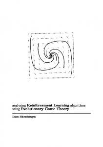
Vk (s) = Vk (s) = !(7)+2!(1) !(7)+2!(2)
Atlanta, July 11, 2010 Options
" !"
100%
terminal state
10
!k(1) – !k(5) !k(7)
5
(log scale, broken at !1)
10
!k(6) 0
10
/ -100
Proof: Us
5
-10
10
0
1000
2000
3000
4000
5000
Iterations (k)
´ & Sutton (UofA) Szepesvari
Off-policy algorithm for options
π(a) > 0
recognize importanc
10
Parameter values, !k (i)
- 10
Recognizers
:+;
s: se a }, correspondingto this function is a.. linearly .. true value function is easily formed by setting(), = O. In all ways, this task seems a favorablecasefor linear function approximation. ´ & Sutton Szepesv ari (UofA) RL Algorithms we apply to this task is a linear method The prediction , gradient-descentform of
July 11, 2010
29 / 45
Defining the objective function Let δt+1 (θ) = Rt+1 + γVθ (Yt+1 ) − Vθ (Xt ) be the TD-error at time t, ϕt = ϕ(Xt ). TD(0) update: θt+1 − θt = αt δt+1 (θt )ϕt . When TD(0) converges, it converges to a unique vector θ∗ that satisfies E [δt+1 (θ∗ )ϕt ] = 0. (TDEQ) Goal: Come up with an objective function such that its optima satisfy (TDEQ). Solution: h i−1 J(θ) = E [δt+1 (θ)ϕt ]> E ϕt ϕ> E [δt+1 (θ)ϕt ] . t
´ & Sutton (UofA) Szepesvari
RL Algorithms
July 11, 2010
31 / 45
Deriving the algorithm h i−1 J(θ) = E [δt+1 (θ)ϕt ]> E ϕt ϕ> E [δt+1 (θ)ϕt ] . t Take the gradient! h i ∇θ J(θ) = −2E (ϕt − γϕ0t+1 )ϕ> t w(θ), where
h i−1 w(θ) = E ϕt ϕ> E [δt+1 (θ)ϕt ] . t
Idea: introduce two sets of weights! θt+1
=
θt + αt · (ϕt − γ · ϕ0t+1 ) · ϕ> t wt
wt+1
=
wt + βt · (δt+1 (θt ) − ϕ> t wt ) · ϕt .
´ & Sutton (UofA) Szepesvari
RL Algorithms
July 11, 2010
32 / 45
GTD2 with linear function approximation
function GTD2(X, R, Y, θ, w) Input: X is the last state, Y is the next state, R is the immediate reward associated with this transition, θ ∈ Rd is the parameter vector of the linear function approximation, w ∈ Rd is the auxiliary weight 1: f ← ϕ[X] 2: f 0 ← ϕ[Y] 3: δ ← R + γ · θ > f 0 − θ > f 4: a ← f > w 5: θ ← θ + α · (f − γ · f 0 ) · a 6: w ← w + β · (δ − a) · f 7: return (θ, w)
´ & Sutton (UofA) Szepesvari
RL Algorithms
July 11, 2010
33 / 45
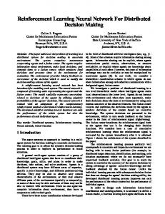
Experimental results
20
RMSPBE
TD 10
GTD2 TDC
GTD
0 0
10
20
30
40
50
Sweeps
Behavior on 7-star example
´ & Sutton (UofA) Szepesvari
RL Algorithms
July 11, 2010
34 / 45
Bibliographic notes and subsequent developments GTD – the original idea (Sutton et al., 2009b) GTD2, a two-timescale version (TDC) (Sutton et al., 2009a). Just replace the update in line 5 by θ ← θ + α · (δ · f − γ · a · f 0 ).
Extension to nonlinear function approximation (Maei et al., 2010) Addresses the issue that TD is unstable when used with nonlinear function approximation Extension to eligibility traces, action-values (Maei and Sutton, 2010) Extension to control (next part!)
´ & Sutton (UofA) Szepesvari
RL Algorithms
July 11, 2010
35 / 45
The problem The methods are “gradient”-like, or “first-order methods” Make small steps in the weight space They are sensitive to: I I I
choice of the step-size initial values of weights eigenvalue spread of the underlying matrix determining the dynamics
Solution proposals: I
I I
Use of adaptive step-sizes (Sutton, 1992; George and Powell, 2006) Normalizing the updates (Bradtke, 1994) Reusing previous samples (Lin, 1992)
Each of them have their own weaknesses
´ & Sutton (UofA) Szepesvari
RL Algorithms
July 11, 2010
37 / 45
The LSTD algorithm In the limit, if TD(0) converges it finds the solution to (∗) E [ ϕt δt+1 (θ) ] = 0. Assume the sample so far is Dn = ((X0 , R1 , Y1 ), (X1 , R2 , Y2 ), . . . , (Xn−1 , Rn , Yn )), Idea: Approximate (*) by
(∗∗)
1 n
Pn−1 t=0
ϕt δt+1 (θ) = 0.
I Stochastic programming: sample average approximation (Shapiro, 2003) I Statistics: Z-estimation (e.g., Kosorok, 2008, Section 2.2.5)
Note: (**) is equivalent to ˆnθ + ˆ −A bn = 0, P 1 Pn−1 0 > ˆ where ˆbn = n1 n−1 t=0 Rt+1 ϕt and An = n t=0 ϕt (ϕt − γϕt+1 ) . ˆ ˆ −1 Solution: θn = A n bn , provided the inverse exists. Least-squares temporal difference learning or LSTD (Bradtke and Barto, 1996). ´ & Sutton (UofA) Szepesvari
RL Algorithms
July 11, 2010
38 / 45
RLSTD(0) with linear function approximation function RLSTD(X, R, Y, C, θ) Input: X is the last state, Y is the next state, R is the immediate reward associated with this transition, C ∈ Rd×d , and θ ∈ Rd is the parameter vector of the linear function approximation 1: f ← ϕ[X] 2: f 0 ← ϕ[Y] 3: g ← (f − γf 0 )> C . g is a 1 × d row vector 4: a ← 1 + gf 5: v ← Cf 6: δ ← R + γ · θ > f 0 − θ > f 7: θ ← θ + δ / a · v 8: C ← C − v g / a 9: return (C, θ)
´ & Sutton (UofA) Szepesvari
RL Algorithms
July 11, 2010
39 / 45
Which one to love? Assumptions Time for computation T is fixed
Samples are cheap to obtain
Some facts How many samples (n) can be processed? Least-squares: n ≈ T/d2 First-order methods: n0 ≈ T/d = nd
Precision after t samples? 1
Least-squares: C1 t− 2 1 First-order: C2 t− 2 C2 > C1
Conclusion Ratio of precisions:
kθn0 0 − θ∗ k C2 − 1 ≈ d 2, kθn − θ∗ k C1
Hence: If C2 /C1 < d1/2 then the first-order method wins, in the other case the least-squares method wins. ´ & Sutton (UofA) Szepesvari
RL Algorithms
July 11, 2010
41 / 45
The choice of the function approximation method
Factors to consider Quality of the solution in the limit of infinitely many samples Overfitting/underfitting “Eigenvalue spread” (decorrelated features) when using first-order methods
´ & Sutton (UofA) Szepesvari
RL Algorithms
July 11, 2010
42 / 45
Error bounds
Consider TD(λ) estimating the value function V. Let Vθ(λ) be the limiting solution. Then kVθ(λ) − Vkµ ≤ √
1 kΠF ,µ V − Vkµ . 1 − γλ
Here γλ = γ(1 − λ)/(1 − λγ) is the contraction modulus of ΠF ,µ T (λ) (Tsitsiklis and Van Roy, 1999; Bertsekas, 2007).
´ & Sutton (UofA) Szepesvari
RL Algorithms
July 11, 2010
43 / 45
Error analysis II ˆ = T (λ) V ˆ − V, ˆ V ˆ : X → R under Define the Bellman ∆(λ) (V) P∞ error (λ) m [m] [m] T = (1 − λ) m=0 λ T , where T is the m-step lookahead Bellman operator.
ˆ ˆ Contraction argument: V − V
≤ 1 ∆(λ) (V)
. ∞
1−γ
∞
ˆ ∆(λ) (V)
What makes small? Error decomposition: ∆(λ) (Vθ(λ) ) = (1 − λ)
X m≥0
X m [r] m [ϕ] λ ∆m + γ (1 − λ) λ ∆m θ(λ) , m≥0
where I I I I I
[r]
∆m = rm − ΠF ,µ rm [ϕ] ∆m = Pm+1 ϕ> − ΠF ,µ Pm+1 ϕ> rm (x) = E [Rm+1 | X0 = x], Pm+1 ϕ> (x) = (Pm+1 ϕ1 (x), . . . , Pm+1 ϕd (x)), Pm ϕi (x) = E [ϕi (Xm ) | X0 = x].
´ & Sutton (UofA) Szepesvari
RL Algorithms
July 11, 2010
44 / 45
For Further Reading Bertsekas, D. P. (2007). Dynamic Programming and Optimal Control, volume 2. Athena Scientific, Belmont, MA, 3 edition. Bradtke, S. J. (1994). Incremental Dynamic Programming for On-line Adaptive Optimal Control. PhD thesis, Department of Computer and Information Science, University of Massachusetts, Amherst, Massachusetts. Bradtke, S. J. and Barto, A. G. (1996). Linear least-squares algorithms for temporal difference learning. Machine Learning, 22:33–57. George, A. P. and Powell, W. B. (2006). Adaptive stepsizes for recursive estimation with applications in approximate dynamic programming. Machine Learning, 65:167–198. Kosorok, M. R. (2008). Introduction to Empirical Processes and Semiparametric Inference. Springer. Lin, L.-J. (1992). Self-improving reactive agents based on reinforcement learning, planning and teaching. Machine Learning, 9:293–321. ´ C., Bhatnagar, S., Silver, D., Precup, D., Maei, H., Szepesvari, and Sutton, R. (2010). Convergent temporal-difference learning with arbitrary smooth function approximation. In NIPS-22, pages 1204–1212. Maei, H. R. and Sutton, R. S. (2010). GQ(λ): A general gradient algorithm for temporal-difference prediction
´ & Sutton (UofA) Szepesvari
learning with eligibility traces. In Baum, E., Hutter, M., and Kitzelmann, E., editors, AGI 2010, pages 91–96. Atlantis Press. Shapiro, A. (2003). Monte Carlo sampling methods. In Stochastic Programming, Handbooks in OR & MS, volume 10. North-Holland Publishing Company, Amsterdam. Sutton, R. S. (1992). Gain adaptation beats least squares. In Proceedings of the 7th Yale Workshop on Adaptive and Learning Systems, pages 161—166. Sutton, R. S., Maei, H. R., Precup, D., Bhatnagar, S., Silver, D., ´ C., and Wiewiora, E. (2009a). Fast Szepesvari, gradient-descent methods for temporal-difference learning with linear function approximation. In Bottou, L. and Littman, M., editors, ICML 2009, pages 993—1000. ACM. ´ C., and Maei, H. R. (2009b). A Sutton, R. S., Szepesvari, convergent O(n) temporal-difference algorithm for off-policy learning with linear function approximation. In Koller, D., Schuurmans, D., Bengio, Y., and Bottou, L., editors, NIPS-21, pages 1609–1616. MIT Press. Tsitsiklis, J. N. and Van Roy, B. (1999). Average cost temporal-difference learning. Automatica, 35(11):1799–1808.
RL Algorithms
July 11, 2010
45 / 45