computational efficiency such that it can be used in real-time and sample efficiency such that it can learn good action-selection policies with limited experience.
Reinforcement Learning in Continuous State and Action Spaces Hado van Hasselt
Abstract Many traditional reinforcement-learning algorithms have been designed for problems with small finite state and action spaces. Learning in such discrete problems can been difficult, due to noise and delayed reinforcements. However, many real-world problems have continuous state or action spaces, which can make learning a good decision policy even more involved. In this chapter we discuss how to automatically find good decision policies in continuous domains. Because analytically computing a good policy from a continuous model can be infeasible, in this chapter we mainly focus on methods that explicitly update a representation of a value function, a policy or both. We discuss considerations in choosing an appropriate representation for these functions and discuss gradient-based and gradient-free ways to update the parameters. We show how to apply these methods to reinforcement-learning problems and discuss many specific algorithms. Amongst others, we cover gradient-based temporal-difference learning, evolutionary strategies, policy-gradient algorithms and (natural) actor-critic methods. We discuss the advantages of different approaches and compare the performance of a state-of-theart actor-critic method and a state-of-the-art evolutionary strategy empirically.
1 Introduction In this chapter, we consider the problem of sequential decision making in continuous domains with delayed reward signals. The full problem requires an algorithm to learn how to choose actions from an infinitely large action space to optimize a noisy delayed cumulative reward signal in an infinitely large state space, where even the outcome of a single action can be stochastic. Desirable properties of such an algorithm include applicability in many different instantiations of the general problem, Hado van Hasselt Centrum Wiskunde en Informatica (CWI, Center for Mathematics and Computer Science) Amsterdam, The Netherlands
1
2
Hado van Hasselt
computational efficiency such that it can be used in real-time and sample efficiency such that it can learn good action-selection policies with limited experience. Because of the complexity of the full reinforcement-learning problem in continuous spaces, many traditional reinforcement-learning methods have been designed for Markov decision processes (MDPs) with small finite state and action spaces. However, many problems inherently have large or continuous domains. In this chapter, we discuss how to use reinforcement learning to learn good action-selection policies in MDPs with continuous state spaces and discrete action spaces and in MDPs where the state and action spaces are both continuous. Throughout this chapter, we assume that a model of the environment is not known. If a model is available, one can use dynamic programming (Bellman, 1957; Howard, 1960; Puterman, 1994; Sutton and Barto, 1998; Bertsekas, 2005, 2007), or one can sample from the model and use one of the reinforcement-learning algorithms we discuss below. We focus mainly on the problem of control, which means we want to find action-selection policies that yield high returns, as opposed to the problem of prediction, which aims to estimate the value of a given policy. For general introductions to reinforcement learning from varying perspectives, we refer to the books by Bertsekas and Tsitsiklis (1996) and Sutton and Barto (1998) and the more recent books by Bertsekas (2007), Powell (2007), Szepesv´ari (2010) and Bus¸oniu et al (2010). Whenever we refer to a chapter, it is implied to be the relevant chapter from the same volume as this chapter. In the remainder of this introduction, we describe the structure of MDPs in continuous domains and discuss three general methodologies to find good policies in such MDPs. We discuss function approximation techniques to deal with large or continuous spaces in Section 2. We apply these techniques to reinforcement learning in Section 3, where we discuss the current state of knowledge for reinforcement learning in continuous domains. This includes discussions on temporal differences, policy gradients, actor-critic algorithms and evolutionary strategies. Section 4 shows the results of an experiment, comparing an actor-critic method to an evolutionary strategy on a double-pole cart pole. Section 5 concludes the chapter.
1.1 Markov Decision Processes in Continuous Spaces A Markov decision process (MDP) is a tuple (S, A, T, R, γ ). In this chapter, the state space S is generally an infinitely large bounded set. More specifically, we assume the state space is a subset of a possibly multi-dimensional Euclidean space, such that S ⊆ RDS , where DS ∈ N is the dimension of the state space. The action space is discrete or continuous and in the latter case we assume A ⊆ RDA , where DA ∈ N is the dimension of the action space.1 We consider two variants: MDPs with continuous states and discrete actions and MDPs where both the states and actions 1
In general, the action space is more accurately represented with a function that maps a state into a continuous set, such that A(s) ⊆ RDA . We ignore this subtlety for conciseness.
Reinforcement Learning in Continuous State and Action Spaces
3
Table 1 Symbols used in this chapter. All vectors are column vectors. DX ∈ {1, 2, . . .} S ⊆ R DS A ⊆ R DA T : S × A × S → [0, 1] R : S×A×S → R γ ∈ [0, 1] V :S→R Q : S×A → R π : S × A → [0, 1] α ∈ R, β ∈ R t ∈N k∈N Φ ⊆ R DΦ φ :S→Φ Θ ⊆ RDΘ θ ∈Θ Ψ ⊆ RDΨ ψ ∈Ψ e ∈ RDΘ n %x% = ∑ x[i]2 ! i=0 % f % = x∈X ( f (x))2 dx ! % f %w = x∈X w(x)( f (x))2 dx
dimension of space X state space action space state-transition function expected-reward function discount factor state value function state-action value function action-selection policy step-size parameters (may depend on state and action) time step episode feature space feature-extraction function parameter space for value functions parameter vector for a value function parameter space for policies parameter vector for a policy eligibility trace vector quadratic norm of vector x = {x[0], . . . , x[n]} quadratic norm of function f : X → R quadratic weighted norm of function f : X → R
are continuous. Often, when we write ‘continuous’ the results hold for ‘large finite’ spaces as well. The notation used in this chapter is summarized in Table 1. The transition function T (s, a, s& ) gives the probability of a transition to s& when action a is performed in s. When the state space is continuous, we can assume the transition function specifies a probability density function (PDF), such that "
S&
T (s, a, s& ) ds& = P(st+1 ∈ S& |st = s and at = a)
denotes the probability that action a in state s results in a transition to a state in the region S& ⊆ S. It is often more intuitive to describe the transitions through a function that describes the system dynamics, such that st+1 = T (st , at ) + ωT (st , at ) , where T : S × A → S is a deterministic transition function that returns the expected next state for a given state-action pair and ωT (s, a) is a zero-mean noise vector with the same size as the state vector. For example, st+1 could be sampled from a Gaussian distribution centered at T (st , at ). The reward function gives the expected reward for any two states and an action. The actual reward can contain noise: rt+1 = R(st , at , st+1 ) + ωR (st , at , st+1 ) , where ωR (s, a, s& ) is a real-valued zero-mean noise term. If ωR and the components of ωT are not uniformly zero at all time steps, the MDP is called stochastic. Oth-
4
Hado van Hasselt
erwise it is deterministic. If T or R is time-dependent, the MDP is non-stationary. In this chapter, we assume stationary MDPs. Since it is commonly assumed that S, A and γ are known, when we refer to a model in this chapter we usually mean (approximations of) T and R. When only the state space is continuous, the action-selection policy is represented by a state dependent probability mass function π : S × A → [0, 1], such that
π (s, a) = P(at = a|st = s) and
∑ π (s, a) = 1
.
a∈A
When the action space is also continuous, π (s) represents a PDF on the action space. The goal of prediction is to find the value of the expected future discounted reward for a given policy. The goal of control is to optimize this value by finding an optimal policy. It is useful to define the following operators Bπ : V → V and B∗ : V → V , where V is the space of all value functions:2 (Bπ V )(s) =
"
π (s, a)
A
(B∗V )(s) = max a
"
S
"
S
# $ T (s, a, s& ) R(s, a, s& ) + γ V (s& ) ds& da ,
(1)
$ # T (s, a, s& ) R(s, a, s& ) + γ V (s& ) ds& ,
In continuous MDPs, the values of a given policy and the optimal value can then be expressed with the Bellman equations V π = Bπ V π and V ∗ = B∗V ∗ . Here V π (s) is the value of performing policy π starting from state s and V ∗ (s) = maxπ V π (s) is the value of the best possible policy. If the action space is finite, the outer integral in equation (1) should be replaced with a summation. In this chapter, we mainly consider discounted MDPs, which means that γ ∈ (0, 1). For control with finite action spaces, action values are often used. The optimal action value for continuous state spaces is given by the Bellman equation % & " & ∗ & & ∗ & (2) Q (s, a) = T (s, a, s ) R(s, a, s ) + γ max Q (s , a ) ds& . S
a&
The idea is that when Q∗ is approximated by Q with sufficient accuracy, we get a good policy by selecting the argument a that maximizes Q(s, a) in each state s. Unfortunately, when the action space is continuous both this selection and the max operator in equation (2) may require finding the solution for a non-trivial optimization problem. We discuss algorithms to deal with continuous actions in Section 3. First, we discuss three general ways to learn good policies in continuous MDPs.
In the literature, these operators are more commonly denoted T π and T ∗ (e.g., Szepesv´ari, 2010), but since we use T to denote the transition function, we choose to use B. 2
Reinforcement Learning in Continuous State and Action Spaces
5
1.2 Methodologies to Solve a Continuous MDP In the problem of control, the aim is an approximation of the optimal policy. The optimal policy depends on the optimal value, which in turn depends on the model of the MDP. In terms of equation (2), the optimal policy is the policy π ∗ that maximizes Q∗ for each state: ∑a π ∗ (s, a)Q∗ (s, a) = maxa Q∗ (s, a). This means that rather than trying to estimate π ∗ directly, we can try to estimate Q∗ , or we can even estimate T and R to construct Q∗ and π ∗ when needed. These observations lead to the following three general methodologies that differ in which part of the solution is explicitly approximated. These methodologies are not mutually exclusive and we will discuss algorithms that use combinations of these approaches. Model Approximation Model-approximation algorithms approximate the MDP and compute the desired policy on this approximate MDP. Since S, A and γ are assumed to be known, this amounts to learning an approximation for the functions T and R.3 Because of the Markov property, these functions only depend on local data. The problem of estimating these functions then translates to a fairly standard supervised learning problem. For instance, one can use Bayesian methods (Dearden et al, 1998, 1999; Strens, 2000; Poupart et al, 2006) to estimate the required model. Learning the model may not be trivial, but in general it is easier than learning the value of a policy or optimizing the policy directly. For a recent survey on model-learning algorithms, see Nguyen-Tuong and Peters (2011). An approximate model can be used to compute a value function. This can be done iteratively, for instance using value iteration or policy iteration (Bellman, 1957; Howard, 1960; Puterman and Shin, 1978; Puterman, 1994). The major drawback of model-based algorithms in continuous-state MDPs is that even if a model is known, in general one cannot easily extract a good policy from the model for all possible states. For instance, value iteration uses an inner loop over the whole state space, which is impossible if this space is infinitely large. Alternatively, a learned model can be used to generate sample runs. These samples can then be used to estimate a value function, or to improve the policy, using one of the methods outlined below. However, if the accuracy of the model is debatable, the resulting policy may not be better than a policy that is based directly on the samples that were used to construct the approximate model. In some cases, value iteration can be feasible, for instance because T (s, a, s& ) is non-zero for only a small number of states s& . Even so, it may be easier to approximate the value directly than to infer the values from an approximate model. For reasons of space, we will not consider model approximation further. Value Approximation In this second methodology, the samples are used to approximate V ∗ or Q∗ directly. Many reinforcement-learning algorithms fall into this category. We discuss value-approximation algorithms in Section 3.1.
3
In engineering, the reward function is usually considered to be known. Unfortunately, this does not make things much easier, since the transition function is usually harder to estimate anyway.
6
Hado van Hasselt
Policy Approximation Value-approximation algorithms parametrize the policy indirectly by estimating state or action values from which a policy can be inferred. Policy-approximation algorithms store a policy directly and try update this policy to approximate the optimal policy. Algorithms that only store a policy, and not a value function, are often called direct policy-search (Ng et al, 1999) or actor-only algorithms (Konda and Tsitsiklis, 2003). Algorithms that store both a policy and a value function are commonly known as actor-critic methods (Barto et al, 1983; Sutton, 1984; Sutton and Barto, 1998; Konda, 2002; Konda and Tsitsiklis, 2003). We will discuss examples of both these approaches. Using this terminology, valuebased algorithms that do not store an explicit policy can be considered critic-only algorithms. Policy-approximation algorithms are discussed in Section 3.2.
2 Function Approximation Before we discuss algorithms to update approximations of value functions or policies, we discuss general ways to store and update an approximate function. General methods to learn a function from data are the topic of active research in the field of machine learning. For general discussions, see for instance the books by Vapnik (1995), Mitchell (1996) and Bishop (2006). In Sections 2.1 and 2.2 we discuss linear and non-linear function approximation. In both cases, the values of the approximate function are determined by a set of tunable parameters. In Section 2.3 we discuss gradient-based and gradient-free methods to update these parameters. Both approaches have often been used in reinforcement learning with considerable success (Sutton, 1988; Werbos, 1989b,a, 1990; Whitley et al, 1993; Tesauro, 1994, 1995; Moriarty and Miikkulainen, 1996; Moriarty et al, 1999; Whiteson and Stone, 2006; Wierstra et al, 2008; R¨uckstieß et al, 2010). Because of space limitations, we will not discuss non-parametric approaches, such as kernel-based methods (see, e.g., Ormoneit and Sen, 2002; Powell, 2007; Bus¸oniu et al, 2010). In this section, we mostly limit ourselves to the general functional form of the approximators and general methods to update the parameters. In order to apply these methods to reinforcement learning, there are a number of design considerations. For instance, we have to decide how to measure how accurate the approximation is. We discuss how to apply these methods to reinforcement learning in Section 3. In supervised learning, a labeled data set is given that contains a number of inputs with the intended outputs for these inputs. One can then answer statistical questions about the process that spawned the data, such as the value of the function that generated the data at unseen inputs. In value-based reinforcement learning, targets may depend on an adapting policy or on adapting values of states. Therefore, targets may change during training and not all methods from supervised learning are directly applicable to reinforcement learning. Nonetheless, many of the same techniques can successfully be applied to the reinforcement learning setting, as long as one is careful about the inherent properties of learning in an MDP. First, we discuss some
Reinforcement Learning in Continuous State and Action Spaces
7
issues on the choice of approximator. This discussion is split into a part on linear function approximation and one on non-linear function approximation.
2.1 Linear Function Approximation We assume some feature-extraction function φ : S → Φ is given that maps states into features in the feature space Φ . We assume Φ ⊆ RDΦ where DΦ is the dimension of the feature space. Often DΦ < DS , which means that the feature vector of a state is smaller than the full representation of the state. This need not hold in general. A discussion about the choice of good features falls outside the scope of this chapter, but see for instance Bus¸oniu et al (2010) for some considerations. A linear function is a simple parametric function that depends on the feature vector. For instance, consider a value-approximating algorithm where the value function is approximated by (3) Vt (s) = θ tT φ (s) . In equation (3) and in the rest of this chapter, θ t ∈ Θ denotes the adaptable parameter vector at time t and φ (s) ∈ Φ is the feature vector of state s. Since the function in equation (3) is linear in the parameters, we refer to it as a linear function approximator. Note that it may be non-linear in the state variables, depending on the feature extraction. In this section, the dimension DΘ of the parameter space is equal to the dimension of the feature space DΦ . This does not necessarily hold for other types of function approximation. Linear function approximators are useful since they are better understood than non-linear function approximators. Applied to reinforcement learning, this has led to a number of convergence guarantees, under various additional assumptions (Sutton, 1984, 1988; Dayan, 1992; Peng, 1993; Dayan and Sejnowski, 1994; Bertsekas and Tsitsiklis, 1996; Tsitsiklis and Van Roy, 1997). From a practical point of view, linear approximators are useful because they are simple to implement and fast to compute. Many problems have large state spaces in which each state can be represented efficiently with a feature vector of limited size. For instance, the double pole cart pole problem that we consider later in this chapter has continuous state variables, and therefore an infinitely large state space. Yet, every state can be represented with a vector with six elements. This means that we would need a table of infinite size, but can suffice with a parameter vector with just six elements if we use (3) with the state variables as features. This reduction of tunable parameters of the value function comes at a cost. It is obvious that not every possible value function can be represented as a linear combination of the features of the problem. Therefore, our solution is limited to the set of value functions that can be represented with the chosen functional form. If one does not know beforehand what useful features are for a given problem, it can be beneficial to use non-linear function approximation, which we discuss in Section 2.2.
8
Hado van Hasselt
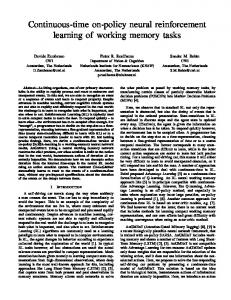
Fig. 1: An elliptical state space is discretized by tile coding with two tilings. For a state located at the X, the two active tiles are shown in light grey. The overlap of these active features is shown in dark grey. On the left, each tiling contains 12 tiles. The feature vector contains 24 elements and 35 different combinations of active features can be encountered in the elliptical state space. On the right, the feature vector contains 13 elements and 34 combinations of active features can be encountered, although some combinations correspond to very small parts of the ellipse.
2.1.1 Discretizing the State Space: Tile Coding A common method to find features for a linear function approximator divides the continuous state space into separate segments and attaches one feature to each segment. A feature is active (i.e., equal to one) if the relevant state falls into the corresponding segment. Otherwise, it is inactive (i.e., equal to zero). An example of such a discretizing method that is often used in reinforcement learning is tile coding (Watkins, 1989; Lin and Kim, 1991; Sutton, 1996; Santamaria et al, 1997; Sutton and Barto, 1998), which is based on the Cerebellar Model Articulation Controller (CMAC) structure proposed by Albus (1971, 1975). In tile coding, the state space is divided into a number of disjoint sets. These sets are commonly called tiles in this context. For instance, one could define N hypercubes such that each hypercube Hn is defined by a Cartesian product Hn = [xn,1 , yn,1 ] × . . . × [xn,DS , yn,DS ], where xn,d is the lower bound of hypercube Hn in state dimension d and yn,d is the corresponding upper bound. Then, a feature φn (s) ∈ φ (s) corresponding to Hn is equal to one when s ∈ Hn and zero otherwise. The idea behind tile coding is to use multiple non-overlapping tilings. If a single tiling contains N tiles, one could use M such tilings to obtain a feature vector of dimension DΦ = MN. In each state, precisely M of these features are then equal to one, while the others are equal to zero. An example with M = 2 tilings and DΦ = 24 features is shown on the left in Figure 1. The tilings do not have to be homogeneous. The right picture in Figure 1 shows a non-homogeneous example with M = 2 tilings and DΦ = 13 features. # $ When M features are active for each state, up to DMΦ different situations can theoretically be represented with DΦ features. This contrasts with the naive approach where only one feature is active for each state, which would only be able to repre-
Reinforcement Learning in Continuous State and Action Spaces
9
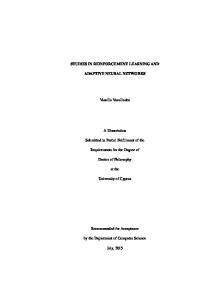
Fig. 2: A reward function and feature mapping. The reward is Markov for the features. If st+1 = st + at with at ∈ {−2, 2}, the feature-transition function is not Markov. This makes it impossible to determine an optimal policy.
4 sent DΦ different #D $ situations with the same number of features. In practice, the upper Φ bound of M will rarely be obtained, since many combinations of active features will not be possible. In both examples in Figure 1, the number of different possible feature vectors is indeed larger than the length smaller than # $ of the feature vector #and 13$ the theoretical upper bound: 24 < 35 < 24 = 276 and 13 < 34 < 2 2 = 78.
2.1.2 Issues with Discretization One potential problem with discretizing methods such as tile coding is that the resulting function that maps states into features is not injective. In other words, φ (s) = φ (s& ) does not imply that s = s& . This means that the resulting feature-space MDP is partially observable and one should consider using an algorithm that is explicitly designed to work on partially observable MDPs (POMDPs). For more on POMDPs, see Chapter ??. In practice, many good results have been obtained with tile coding, but the discretization and the resulting loss of the Markov property imply that most convergence proofs for ordinary reinforcement-learning algorithms do not apply for the discretized state space. This holds for any function approximation that uses a feature space that is not an injective function of the Markov state space. Intuitively, this point can be explained with a simple example. Consider a state space S = R that is discretized such that φ (s) = (1, 0, 0)T when s ≤ −2, φ (s) = (0, 1, 0)T when −2 < s < 2 and φ (s) = (0, 0, 1)T when s ≥ 2. The action space is A = {−2, 2}, the transition function is st+1 = st + at and the initial state is s0 = 1. The reward is defined by rt+1 = 1 if st ∈ (−2, 2) and rt+1 = −1 otherwise. The reward function and the feature mapping are shown in Figure 2. In this MDP, it is optimal to jump back and forth between the states s = −1 and s = 1. However, if we observe the feature vector (0, 1, 0)T , we can not know if we are in s = −1 or s = 1 and we cannot determine the optimal action. Another practical issue with methods such as tile coding is related to the step-size parameter that many algorithms use. For instance, in many algorithms the parameters of a linear function approximator are updated with an update akin to
4
Note that 1 < M < DΦ implies that DΦ
1/M. This can cause divergence of the parameters. Conversely, if the euclidean norm %φ (s)% of the feature vector is often small, the change to the value function may be smaller than intended. This issue can occur for any feature space and linear function approximation, since then the effective step sizes in (5) are used for the update to the value function. This indicates that it can be a good idea to scale the step size appropriately, by using
α˜ t (st ) = αt (st )/%φ (st )% , where α˜ t (st ) is the scaled step size.5 This scaled step size can prevent unintended small as well as unintended large updates to the values. Φ In general, it is often a good idea to make sure that |φ (s)| = ∑D k φk (s) ≤ 1 for all s. For instance, in tile coding we could set the value of active features equal to 1/M instead of to 1. In general, function approximators for which this property holds include so called averagers (Gordon, 1995) and interpolators (Szepesv´ari and Smart, 2004). Such feature representations have good convergence properties, because they are non-expansions, which means that maxs |φ (s)T θ − φ (s)T θ & | ≤ maxk |θk − θk& | for any feature vector φ (s) and any two parameter vectors θ and θ & . A non-expansive function makes it easier to prove that an algorithm iteratively improves its solution in expectation through a so-called contraction mapping (Gordon, 1995; Littman and Szepesv´ari, 1996; Bertsekas and Tsitsiklis, 1996; Bertsekas, 2007; Szepesv´ari, 2010; Bus¸oniu et al, 2010). Algorithms that implement a contraction mapping eventually reach an optimal solution and can be guaranteed not to diverge, for instance by updating their parameters to infinitely high values.
5
One can safely define α˜ t (st ) = 0 if %φ (st )% = 0, since in that case update (4) would not change the parameters anyway.
Reinforcement Learning in Continuous State and Action Spaces
11
A final issue with discretization is that it introduces discontinuities in the function. If the input changes a small amount, the approximated value may change a fairly large amount if the two inputs fall into different segments of the input space.
2.1.3 Fuzzy Representations Some of the issues with discretization can be avoided by using a function that is piece-wise linear, rather than piece-wise constant. One way to do this, is by using so-called fuzzy sets (Zadeh, 1965; Klir and Yuan, 1995; Babuska, 1998). A fuzzy set is a generalization of normal sets to fuzzy membership. This means that elements can partially belong to a set, instead of just the possibilities of truth or falsehood. A common example of fuzzy sets is the division of temperature into ‘cold’ and ‘warm’. There is a gradual transition between cold and warm, so often it is more natural to say that a certain temperature is partially cold and partially warm. In reinforcement learning, the state or state-action space can be divided into fuzzy sets. Then, a state may belong partially to the set defined by feature φi and partially to the set defined by feature φ j . For instance, we may have φi (s) = 0.1 and φ j (s) = 0.3. An advantage of this view is that it is quite natural to assume that ∑k φk (s) ≤ 1, since each part of an element can belong to only one set. For instance, something cannot be fully warm and fully cold at the same time. It is possible to define the sets such that each combination of feature activations corresponds precisely to one single state, thereby avoiding the partial-observability problem sketched earlier. A common choice is to use triangular functions that are equal to one at the center of the corresponding feature and decay linearly to zero for states further from the center. With some care, such features can be constructed such that they span the whole state space and ∑k φk (s) ≤ 1 for all states. A full treatment of fuzzy reinforcement learning falls outside the scope of this chapter. References that make the explicit connection between fuzzy logic and reinforcement learning include Berenji and Khedkar (1992); Berenji (1994); Lin and Lee (1994); Glorennec (1994); Bonarini (1996); Jouffe (1998); Zhou and Meng (2003) and Bus¸oniu et al (2008, 2010). A drawback of fuzzy sets is that these sets still need to be defined beforehand, which may be difficult.
2.2 Non-linear Function Approximation The main drawback of linear function approximation compared to non-linear function approximation is the need for good informative features.6 The features are often assumed to be hand-picked beforehand, which may require domain knowledge. Even if convergence in the limit to an optimal solution is guaranteed, this solution is only optimal in the sense that it is the best possible linear function of the given 6
Non-parametric approaches somewhat alleviate this point, but are harder to analyze in general. A discussion on such methods falls outside the scope of this chapter.
12
Hado van Hasselt
features. Additionally, while less theoretical guarantees can be given, nice empirical results have been obtained by combining reinforcement-learning algorithms with non-linear function approximators, such as neural networks (Haykin, 1994; Bishop, 1995, 2006; Ripley, 2008). Examples include Backgammon (Tesauro, 1992, 1994, 1995), robotics (Anderson, 1989; Lin, 1993; Touzet, 1997; Coulom, 2002) and elevator dispatching (Crites and Barto, 1996, 1998). In a parametric non-linear function approximator, the function that should be optimized is represented by some predetermined parametrized function. For instance, for value-based algorithms we may have Vt (s) = V (φ (s), θt ) .
(6)
Here the size of θt ∈ Θ is not necessarily equal to the size of φ (s) ∈ Φ . For instance, V may be a neural network where θ t is a vector with all its weights at time t. Often, the functional form of V is fixed. However, it is also possible to change the structure of the function during learning (e.g., Stanley and Miikkulainen, 2002; Taylor et al, 2006; Whiteson and Stone, 2006; Bus¸oniu et al, 2010). In general, a non-linear function approximator may approximate an unknown function with better accuracy than a linear function approximator that uses the same input features. In some cases, it is even possible to avoid defining features altogether by using the state variables as inputs. A drawback of non-linear function approximation in reinforcement learning is that less convergence guarantees can be given. In some cases, convergence to a local optimum can be assured (e.g., Maei et al, 2009), but in general the theory is less well developed than for linear approximation.
2.3 Updating Parameters Some algorithms allow for the closed-form computation of parameters that best approximate the desired function, for a given set of experience samples. For instance, when TD-learning is coupled with linear function approximation, leastsquares temporal-difference learning (LSTD) (Bradtke and Barto, 1996; Boyan, 2002; Geramifard et al, 2006) can be used to compute parameters that minimize the empirical temporal-difference error over the observed transitions. However, for nonlinear algorithms such as Q-learning or when non-linear function approximation is used, these methods are not applicable and the parameters should be optimized in a different manner. Below, we explain how to use the two general techniques of gradient descent and gradient-free optimization to adapt the parameters of the approximations. These procedures can be used with both linear and non-linear approximation and they can be used for all three types of functions: models, value functions and policies. In Section 3, we discuss reinforcement-learning algorithms that use these methods. We will not discuss Bayesian methods in any detail, but such methods can be used to learn the probability distributions of stationary functions, such as the reward and
Reinforcement Learning in Continuous State and Action Spaces
13
1: input: differentiable function E : RN × RP → R to be minimized, step size sequence αt ∈ [0, 1], initial parameters θ0 ∈ RP 2: output: a parameter vector θ such that E is small 3: for all t ∈ {1, 2, . . .} do 4: Observe xt , E(xt , θt ) 5: Calculate gradient: ∇θ E(xt , θt ) = 6:
%
∂ ∂ E(xt , θt ), . . . , E(xt , θt ) ∂ θt [1] ∂ θt [P]
&T
.
Update parameters:
θ t+1 = θ t − αt ∇θ E(x, θt )
Algorithm 1: Stochastic gradient descent
transition functions of a stationary MDP. An advantage of this is that the exploration of an online algorithm can choose actions to increase the knowledge of parts of the model that have high uncertainty. Bayesian methods are somewhat less suited to learn the value of non-stationary functions, such as the value of a changing policy. For more general information about Bayesian inference, see for instance Bishop (2006). For Bayesian methods in the context of reinforcement learning, see Dearden et al (1998, 1999); Strens (2000); Poupart et al (2006) and Chapter ??.
2.3.1 Gradient Descent A gradient-descent update follows the direction of the negative gradient of some parametrized function that we want to minimize. The gradient of a parametrized function is a vector in parameter space that points in the direction in which the function increases, according to a first-order Taylor expansion. Put more simply, if the function is smooth and we change the parameters a small amount in the direction of the gradient, we expect the function to increase slightly. The negative gradient points in the direction in which the function is expected to decrease, so moving the parameters in this direction should result in a lower value for the function. Algorithm 1 shows the basic algorithm, where for simplicity a real-valued parametrized function E : RN × RP → R is considered. The goal is to make the output of this function small. To do this, the parameters of θ ∈ RDΘ of E are updated in the direction of the negative gradient. The gradient ∇θ E(x, θ ) is a column vector whose components are the derivatives of E to the elements of the parameter vector θ , calculated at the input x. Because the gradient only describes the local shape of the function, this algorithm can end up in a local minimum. Usually, E is an error measure such as a temporal-difference or a prediction error. For instance, consider a parametrized approximate reward function R¯ : S×A×RP → ¯ t , at , θt )−rt+1 )2 . R and a sample (st , at , rt+1 ). Then, we might use E(st , at , θt ) = (R(s If the gradient is calculated over more than one input-output pair at the same time, the result is the following batch update
14
Hado van Hasselt
θ t+1 = θ t − αt ∑ ∇θ Ei (xi , θt ) , i
where Ei (xi , θt ) is the error for the i th input xi and αt ∈ [0, 1] is a step-size parameter. If the error is defined over only a single input-output pair, the update is called a stochastic gradient descent update. Batch updates can be used in offline algorithms, while stochastic gradient descent updates are more suitable for online algorithms. There is some indication that often stochastic gradient descent converges faster than batch gradient descent (Wilson and Martinez, 2003). Another advantage of stochastic gradient descent over batch learning is that it is straightforward to extend online stochastic gradient descent to non-stationary targets, for instance if the policy changes after an update. These features make online gradient methods quite suitable for online reinforcement learning. In general, in combination with reinforcement learning convergence to an optimal solution is not guaranteed, although in some cases convergence to a local optimum can be proven (Maei et al, 2009). In the context of neural networks, gradient descent is often implemented through backpropagation (Bryson and Ho, 1969; Werbos, 1974; Rumelhart et al, 1986), which uses the chain rule and the layer structure of the networks to efficiently calculate the derivatives of the network’s output to its parameters. However, the principle of gradient descent can be applied to any differentiable function. In some cases, the normal gradient is not the best choice. More formally, a problem of ordinary gradient descent is that the distance metric in parameter space may differ from the distance metric in function space, because of interactions between the parameters. Let dθ ∈ RP denote a vector in parameter space. The euclidean norm of this vector is %dθ % = dθ T dθ . However, if the parameter space is a curved space—known as a Riemannian manifold—it is more appropriate to use dθ T G dθ where G is a P×P positive semi-definite matrix. With this weighted distance metric, the direction of steepest descent becomes ˜ θ E(x, θ ) = G−1 ∇θ E(x, θ ) , ∇ which is known as the natural gradient (Amari, 1998). In general, the best choice for matrix G depends on the functional form of E. Since E is not known in general, G will usually need to be estimated. Natural gradients have a number of advantages. For instance, the natural gradient is invariant to transformations of the parameters. In other words, when using a natural gradient the change in our function does not depend on the precise parametrization of the function. This is somewhat similar to our observation in Section 2.1.2 that we can scale the step size to tune the size of the step in value space rather than in parameter space. Only here we consider the direction of the update to the parameters, rather than its size. Additionally, the natural gradient avoids plateaus in function space, often resulting in faster convergence. We discuss natural gradients in more detail when we discuss policy-gradient algorithms in Section 3.2.1.
Reinforcement Learning in Continuous State and Action Spaces
15
2.3.2 Gradient-Free Optimization Gradient-free methods are useful when the function that is optimized is not differentiable or when it is expected that many local optima exist. Many general global methods for optimization exist, including evolutionary algorithms (Holland, 1962; Rechenberg, 1971; Holland, 1975; Schwefel, 1977; Davis, 1991; B¨ack and Schwefel, 1993), simulated annealing (Kirkpatrick, 1984), particle swarm optimization (Kennedy and Eberhart, 1995) and cross-entropy optimization (Rubinstein, 1999; Rubinstein and Kroese, 2004). Most of these methods share some common features that we will outline below. We focus on cross-entropy and a subset of evolutionary algorithms, but the other approaches can be used quite similarly. For introductions to evolutionary algorithms, see the books by B¨ack (1996) and Eiben and Smith (2003). For a more extensive account on evolutionary algorithms in reinforcement learning, see Chapter ??. We give a short overview of how such algorithms work. All the methods described here use a population of solutions. Traditional evolutionary algorithms create a population of solutions and adapt this population by selecting some solutions, recombining these and possibly mutating the result. The newly obtained solutions then replace some or all of the solutions in the old population. The selection procedure typically takes into account the fitness of the solutions, such that solutions with higher quality have a larger probability of being used to create new solutions. Recently, it has become more common to adapt the parameters of a probability distribution that generates solutions, rather than to adapt the solutions themselves. This approach is used in so-called evolutionary strategies (B¨ack, 1996; Beyer and Schwefel, 2002). Such approaches generate a population, but use the fitness of the solutions to adapt the parameters of the generating distribution, rather than the solutions themselves. A new population is then obtained by generating new solutions from the adapted probability distribution. Some specific algorithms include the following. Covariance matrix adaptation evolution strategies (CMA-ES) (Hansen and Ostermeier, 2001) weigh the sampled solutions according to their fitness and use the weighted mean as the mean of the new distribution. Natural evolutionary strategies (NES) (Wierstra et al, 2008; Sun et al, 2009) use all the generated solutions to estimate the gradient of the parameters of the generating function, and then use natural gradient ascent to improve these parameters. Cross-entropy optimization methods (Rubinstein and Kroese, 2004) simply select the m solutions with the highest fitness—where m is a parameter—and use the mean of these solutions to find a new mean for the distribution.7 7
According to this description, cross-entropy optimization can be considered an evolutionary strategy similar to CMA-ES, using a special weighting that weighs the top m solutions with 1/m and the rest with zero. There are more differences between the known algorithmic implementations however, most important of which is perhaps the more elegant estimation of the covariance matrix of the newly formed distribution by CMA-ES, aimed to increase the probability of finding new solutions with high fitness. Some versions of cross-entropy add noise to the variance to prevent premature convergence (e.g., Szita and L¨orincz, 2006), but the theory behind this seems less well-developed than covariance estimation used by CMA-ES.
16
Hado van Hasselt
1: input: parametrized population PDF p : RK × RP → R, fitness function f : RP → R, initial parameters ζ0 ∈ RK , population size n 2: output: a parameter vector ζ such that if θ ∼ p(ζ , ·) then f (θ ) is large with high probability 3: for all t ∈ {1, 2, . . .} do 4: Construct population Θt = {θ¯1 , θ¯2 , . . . , θ¯n }, where θ¯i ∼ p(ζt , ·) 5: Use the fitness scores f (θ¯i ) to compute ζt+1 such that E{ f (θ )|ζt+1 } > E{ f (θ )|ζt }
Algorithm 2: A generic evolutionary strategy
A generic evolutionary strategy is shown in Algorithm 2. The method to compute the next parameter setting ζt+1 for the generating function in line 5 differs between algorithms. However, all attempt to increase the expected fitness such that E{ f (θ )|ζt+1 } is higher than the expected fitness of the former population E{ f (θ )|ζt }. These expectations are defined by E{ f (θ )|ζ } =
"
RP
p(ζ , θ ) f (θ ) d θ .
Care should be taken that the variance of the distribution does not become too small too quickly, in order to prevent premature convergence to sub-optimal solutions. A simple way to do this, is by using a step-size parameter (Rubinstein and Kroese, 2004) on the parameters in order to prevent from too large changes per iteration. More sophisticated methods to prevent premature convergence include the use of the natural gradient by NES, and the use of enforced correlations between the covariance matrices of consecutive populations by CMA-ES. No general guarantees can be given concerning convergence to the optimal solution for evolutionary strategies. Convergence to the optimal solution for nonstationary problems, such as the control problem in reinforcement learning, seems even harder to prove. Despite this lack of guarantees, these methods can perform well in practice. The major bottleneck is usually that the computation of the fitness can be both noisy and expensive. Additionally, these methods have been designed mostly with stationary optimization problems in mind. Therefore, they are more suited to optimize a policy using Monte Carlo samples than to approximate the value of the unknown optimal policy. In Section 4, we compare the performance of CMA-ES and an actor-critic temporal-difference approach. The gradient-free methods mentioned above all fall into a category known as metaheuristics (Glover and Kochenberger, 2003). These methods iteratively search for good candidate solutions, or a distribution that generates these. Another approach is to construct an easier solvable (e.g., quadratic) model of the function that is to be optimized and then maximize this model analytically (see, e.g., Powell, 2002, 2006; Huyer and Neumaier, 2008). New samples can be iteratively chosen to improve the approximate model. We do not know any papers that have used such methods in a reinforcement learning context, but the sample-efficiency of such On a similar note, it has recently been shown that CMA-ES and NES are equivalent except for some differences in the proposed implementation of the algorithms (Akimoto et al, 2011).
Reinforcement Learning in Continuous State and Action Spaces
17
methods in high-dimensional problems make them an interesting direction for future research.
3 Approximate Reinforcement Learning In this section we apply the general function approximation techniques described in Section 2 to reinforcement learning. We discuss some of the current state of the art in reinforcement learning in continuous domains. As mentioned earlier in this chapter, we will not discuss the construction of approximate models because even if a model is known exact planning is often infeasible in continuous spaces.
3.1 Value Approximation In value-approximation algorithms, experience samples are used to update a value function that gives an approximation of the current or the optimal policy. Many reinforcement-learning algorithms fall into this category. Important differences between algorithms within this category is whether they are on-policy or off-policy and whether they update online or offline. Finally, a value-approximation algorithm may store a state-value function V : S → R, or an action-value function Q : S × A → R, or even both (Wiering and van Hasselt, 2009). We will explain these properties and give examples of algorithms for each combination of properties. On-policy algorithms approximate the state-value function V π or the action-value function Qπ , which represent the value of the policy π that they are currently following. Although the optimal policy π ∗ is unknown initially, such algorithms can eventually approximate the optimal value function V ∗ or Q∗ by using policy iteration, which improves the policy between evaluation steps. Such policy improvements may occur as often as each time step. Off-policy algorithms can learn about the value of a different policy than the one that is being followed. This is useful, as it means we do not have to follow a (near-) optimal policy to learn about the value of the optimal policy. Online algorithms adapt their value approximation after each observed sample. Offline algorithms operate on batches of samples. Usually, online algorithms require much less computation per sample, whereas offline algorithms require less samples to reach a similar accuracy of the approximation. Online on-policy algorithms include temporal-difference (TD) algorithms, such as TD-learning (Sutton, 1984, 1988), Sarsa (Rummery and Niranjan, 1994; Sutton and Barto, 1998) and Expected-Sarsa (van Seijen et al, 2009). Offline on-policy algorithms include least-squares approaches, such as leastsquared temporal difference (LSTD) (Bradtke and Barto, 1996; Boyan, 2002; Geramifard et al, 2006), least-squares policy evaluation (LSPE) (Nedi´c and Bertsekas, 2003) and least-squares policy iteration (LSPI) (Lagoudakis and Parr, 2003). Be-
18
Hado van Hasselt
cause of limited space we will not discuss least-squares approaches in this chapter, but see Chapter ?? of this volume. Arguably the best known model-free online off-policy algorithm is Q-learning (Watkins, 1989; Watkins and Dayan, 1992). Its many derivatives include Perseus (Spaan and Vlassis, 2005), Delayed Q-learning (Strehl et al, 2006) and Bayesian Qlearning (Dearden et al, 1998; see also Chapter ??). All these variants try to estimate the optimal policy through use of some variant of the Bellman optimality equation. In general, off-policy algorithms need not estimate the optimal policy, but can also approximate an arbitrary other policy (Precup et al, 2000; Precup and Sutton, 2001; Sutton et al, 2008; van Hasselt, 2011, Section 5.4). Offline variants of Q-learning include fitted Q-iteration (Ernst et al, 2005; Riedmiller, 2005; Antos et al, 2008a). An issue with both the online and the offline variants of Q-learning is that noise in the value approximations, due to the stochasticity of the problem and the limitations of the function approximator, can result a structural overestimation bias. In short, the value of maxa Qt (s, a), as used by Q-learning, may—even in expectancy—be far larger than maxa Q∗ (s, a). This bias can severely slow convergence of Q-learning, even in tabular settings (van Hasselt, 2010) and if care is not taken with the choice of function approximator, it may result in divergence of the parameters (Thrun and Schwartz, 1993). A partial solution for this bias is given by the Double Q-learning algorithm (van Hasselt, 2010), where two action-value functions produce an estimate which may underestimate maxa Q∗ (s, a), but is bounded in expectancy. Many of the aforementioned algorithms can be used both online and offline, but are better suited for either of these approaches. For instance, fitted Q-iteration usually is used as an offline algorithm, since the algorithm is considered too computationally expensive to be run after each sample. Conversely, online algorithms can store the observed samples are reuse these as if they were observed again in a form of experience replay (Lin, 1992). The least-squares and fitted variants are usually used as offline versions of temporal-difference algorithms. There are exceptions however, such as the online incremental LSTD algorithm (Geramifard et al, 2006, 2007). If the initial policy does not easily reach some interesting parts of the statespace, online algorithms have the advantage that the policy is usually updated more quickly, because value updates are not delayed until a sufficiently large batch of samples is obtained. This means that online algorithms are sometimes more sampleefficient in control problems. In the next two subsections, we discuss in detail some online value-approximation algorithms that use a gradient-descent update on a predefined error measure.
3.1.1 Objective Functions In order to update a value with gradient descent, we must choose some measure of error that we can minimize. This measure is often referred to as the objective function. To be able to reason more formally about these objective functions, we introduce the concepts of function space and projections. Recall that V is the space of value functions, such that V ∈ V . Let F ⊆ V denote the function space of rep-
Reinforcement Learning in Continuous State and Action Spaces
19
resentable functions for some function approximator. Intuitively, if F contains a large subset of V , the function is flexible and can accurately approximate many value functions. However, it may be prone to overfitting of the perceived data and it may be slow to update since usually a more flexible function requires more tunable parameters. Conversely, if F is small compared to V , the function is not very flexible. For instance, the function space of a linear approximator is usually smaller than that of a non-linear approximator. A parametrized function has a parameter vector θ = {θ [1], . . . , θ [DΘ ]} ∈ RDΘ that can be adjusted during training. The function space is then defined by ( ' F = V (·, θ )|θ ∈ RDΘ . From here on further, we denote parametrized value functions by Vt if we want to stress the dependence on time and by V θ if we want to stress the dependence on the parameters. By definition, Vt (s) = V (s, θt ) and V θ (s) = V (s, θ ). A projection Π : V → F is an operator that maps a value function to the closest representable function in F , under a certain norm. This projection is defined by %V − Π V %w = min %V − v%w = min %V −V θ %w , θ
v∈F
where % · %w is a weighted norm. We assume the norm is quadratic, such that %V −V θ %w =
"
s∈S
) *2 w(s) V (s) −V θ (s) ds .
This means that the projection is determined by the functional form of the approximator and the weights of the norm. Let B = Bπ or B = B∗ , depending on whether we are approximating the value of a given policy, or the value of the optimal policy. It is often not possible to find a parameter vector that fulfills the Bellman equations V θ = BV θ for the whole state space exactly, because the value BV θ may not be representable with the chosen function. Rather, the best we can hope for is a parameter vector that fulfills V θ = Π BV θ .
(7)
This is called the projected Bellman equation; Π projects the outcome of the Bellman operator back to the space that is representable by the function approximation. In some cases, it is possible to give a closed form expression for the projection (Tsitsiklis and Van Roy, 1997; Bertsekas, 2007; Szepesv´ari, 2010). For instance, consider a finite state space with N states and a linear function Vt (s) = θ T φ (s), where DΘ = DΦ , N. Let ps = P(st = s) denote the expected steady-state probabilities of sampling each state and store these values in a diagonal N × N matrix P. We assume the states are always sampled according to these fixed probabilities. Finally, the N × DΦ matrix Φ holds the feature vectors for all states in its rows, such that Vt = Φθt and Vt (s) = Φs θt = θtT φ (s). Then, the projection operator can be represented by the N × N matrix
20
Hado van Hasselt
Π = Φ Φ T PΦ #
$−1
ΦT P .
(8)
The inverse exists if the features are linearly independent, such that Φ has rank DΦ . With this definition Π Vt = Π Φθt = Φθt = Vt , but Π BVt -= BVt , unless BVt can be expressed as a linear function of the feature vectors. A projection matrix as defined in (8) is used in the analysis and in the derivation of several algorithms (Tsitsiklis and Van Roy, 1997; Nedi´c and Bertsekas, 2003; Bertsekas et al, 2004; Sutton et al, 2008, 2009; Maei and Sutton, 2010). We discuss some of these in the next section.
3.1.2 Gradient Temporal-Difference Learning We generalize standard temporal-difference learning (TD-learning) (Sutton, 1984, 1988) to a gradient update on the parameters of a function approximator. The tabular TD-learning update is Vt+1 (st ) = Vt (st ) + αt (st )δt , where δt = rt+1 + γ Vt (st+1 ) −Vt (st ) and αt (s) ∈ [0, 1] is a step-size parameter. When TD-learning is used to estimate the value of a given stationary policy under onpolicy updates the value function converges when the feature vectors are linearly independent (Sutton, 1984, 1988). Later it was shown that TD-learning also converges when eligibility traces are used and when the features are not linearly independent (Dayan, 1992; Peng, 1993; Dayan and Sejnowski, 1994; Bertsekas and Tsitsiklis, 1996; Tsitsiklis and Van Roy, 1997). More recently, variants of TD-learning were proposed that converge under off-policy updates (Sutton et al, 2008, 2009; Maei and Sutton, 2010). We discuss these variants below. A limitation of most aforementioned results is that they apply only to the prediction setting. Recently some work has been done to extend the analysis to the control setting. This has led to the Greedy-GQ algorithm, which extends Q-learning to linear function approximation without the danger of divergence, under some conditions (Maei et al, 2010). When the state values are stored in a table, TD-learning can be interpreted as a stochastic gradient-descent update on the one-step temporal-difference error E(st ) =
1 1 (rt+1 + γ Vt (st+1 ) −Vt (st ))2 = (δt )2 . 2 2
(9)
If Vt is a parametrized function such that Vt (s) = V (s, θt ), the negative gradient with respect to the parameters is given by −∇θ E(st , θ ) = − (rt+1 + γ Vt (st+1 ) −Vt (st )) ∇θ (rt+1 + γ Vt (st+1 ) −Vt (st )) . Apart from the state and the parameters, the error depends on the MDP and the policy. We do not specify these dependencies explicitly to avoid cluttering the notation. A direct implementation of gradient descent based on the error in (9) would adapt the parameters to move Vt (s) closer to rt+1 + γ Vt (st+1 ) as desired, but would also move γ Vt (st+1 ) closer to Vt (st ) − rt+1 . Such an algorithm is called a residualgradient algorithm (Baird, 1995). Alternatively, we can interpret rt+1 + γ Vt (st+1 ) as
Reinforcement Learning in Continuous State and Action Spaces
21
a stochastic approximation for V π that does not depend on θ . Then, the negative gradient is (Sutton, 1984, 1988) −∇θ Et (st , θ ) = (rt+1 + γ Vt (st+1 ) −Vt (st )) ∇θ Vt (st ) . This implies the parameters can be updated as
θ t+1 = θ t + αt (st )δt ∇θ Vt (st ) .
(10)
This is the conventional TD learning update and it usually converges faster than the residual-gradient update (Gordon, 1995, 1999). For linear function approximation, for any θ we have ∇θ Vt (st ) = φ (st ) and we obtain the same update as was shown earlier for tile coding in (4). Similar updates for action-value algorithms are obtained by replacing ∇θ Vt (st ) in (10) with ∇θ Qt (st , at ) and using, for instance
δt = rt+1 + γ max Qt (st+1 , a) − Qt (st , at ) , or a
δt = rt+1 + γ Qt (st+1 , at+1 ) − Qt (st , at ) , for Q-learning and Sarsa, respectively. We can incorporate accumulating eligibility traces with trace parameter λ with the following two equations (Sutton, 1984, 1988): et+1 = λ γ et + ∇θ Vt (st ) , θ t+1 = θ t + αt (st )δt et+1 , where e ∈ RDΦ is a trace vector. Replacing traces (Singh and Sutton, 1996) are less straightforward, although the suggestion by Fr¨amling (2007) seem sensible: et+1 = max(λ γ et , ∇θ Vt (st )) , since this corresponds nicely to the common practice for tile coding and this update reduces to the conventional replacing traces update when the values are stored in a table. However, a good theoretical justification for this update is still lacking. Parameters updated with (10) may diverge when off-policy updates are used. This holds for any temporal-difference method with λ < 1 when we use linear (Baird, 1995) or non-linear function approximation (Tsitsiklis and Van Roy, 1996). In other words, if we sample transitions from a distribution that does not comply completely to the state-visit probabilities that would occur under the estimation policy, the parameters of the function may diverge. This is unfortunate, because in the control setting ultimately we want to learn about the unknown optimal policy. Recently, a class of algorithms has been proposed to deal with this issue (Sutton et al, 2008, 2009; Maei et al, 2009; Maei and Sutton, 2010). The idea is to perform a stochastic gradient-descent update on the quadratic projected temporal difference: 1 1 E(θ ) = %Vt − Π BVt %P = 2 2
"
s∈S
P(s = st )(Vt (s) − Π BVt (s))2 ds .
(11)
22
Hado van Hasselt
In contrast with (9), this error does not depend on the time step or the state. The norm in (11) is weighted according to the state probabilities that are stored in the diagonal matrix P, as described in Section 3.1.1. If we minimize (11), we reach the fixed point in (7). To do this, we rewrite the error to E(θt ) =
# ' ($−1 1 E {δt ∇θ Vt (s)} , (E {δt ∇θ Vt (s)})T E ∇θ Vt (s)∇θT Vt (s) 2
(12)
where it is assumed that the inverse exists (Maei et al, 2009). The expectancies are taken over the state probabilities in P. The error is the product of multiple expected values. These expected values can not be sampled from a single experience, because then the samples would be correlated. This can be solved by updating an additional parameter vector. We use the shorthands φ = φ (st ) and φ & = φ (st+1 ) and we assume linear function approximation. Then ∇θ Vt (st ) = φ and we get ' (# ' ($−1 −∇θ E(θt ) = E (φ − γφ & )φ T E φ φ T E {δt φ } ( ' & T ≈ E (φ − γφ )φ w ,
where wt ∈ RDΦ is an additional parameter vector. This vector should approximate # ' T ($−1 E φφ E {δt φ }, which can be done with the update # $ wt+1 = wt + βt (st ) δt − φ T wt φ ,
where βt (st ) ∈ [0, 1] is a step-size parameter. Then there is only one expected value left to approximate, which can be done with a single sample. This leads to the update # $# $ θ t+1 = θ t + αt (st ) φ − γφ & φ T wt , which is called the GTD2 (Gradient Temporal-Difference Learning, version 2) algorithm (Sutton et al, 2009). One can also write the gradient in a slightly different manner to obtain the similar TDC algorithm, which is defined as: # # $$ , θ t+1 = θ t + αt (st ) δt φ − γφ & φ T wt
where wt is updated as above. This algorithm is named TD with gradient correction (TDC), because the update to the primary parameter vector θt is equal to (10), except for a correction term. This term prevents divergence of the parameters when offpolicy updates are used. Both GTD2 and TDC can be shown to minimize (12), if the states are sampled according to P. The difference with ordinary TD-learning is that these algorithms also converge when the probabilities in P differ from those that result from following the policy π , whose value we are estimating. This is useful for instance when we have access to a simulator that allows us to sample the states in any order, while π would spend much time in uninteresting states. When non-linear smooth function approximators are used, it can be proven that similar algorithms reach local optima (Maei et al, 2009). The updates for the nonlinear algorithms are similar to the ones above, with another correction term. The
Reinforcement Learning in Continuous State and Action Spaces
23
updates can be extended to a form of Q-learning in order to learn action values with eligibility traces. The resulting GQ(λ ) algorithm is off-policy and converges to the value of a given estimation policy, even when the algorithm follows a different behavior policy (Maei and Sutton, 2010). The methods can be extended to control problems (Maei et al, 2010) with a greedy non-stationary estimation policy, although it is not yet clear how well the resulting Greedy-GQ algorithm performs in practice. Although these theoretic insights and the resulting algorithms are promising, in practice the TD update in (10) is still the better choice in on-policy settings. Additionally, an update akin to (10) for Q-learning often results in good policies, although convergence can not be guaranteed in general. Furthermore, for specific functions— such as the earlier mentioned averagers—Q-learning does converge (Szepesv´ari and Smart, 2004). In practice, many problems do not have the precise characteristics that result in divergence of the parameters. Finally, the convergence guarantees are mainly limited to the use of samples from fixed steady-state probabilities. If we can minimize the so-called Bellman residual error E(θt ) = %V − BV %P , this automatically minimizes the projected temporal-difference error in (11). Using (δt )2 as a sample for this error (with B = Bπ ) leads to a biased estimate, but other approaches have been proposed that use this error (Antos et al, 2008b; Maillard et al, 2010). It is problem-dependent whether minimizing the residual error leads to better results than minimizing the projected error (Scherrer, 2010). It is non-trivial to extend the standard online temporal-difference algorithms such as Q-learning to continuous action spaces. Although we can construct an estimate of the value for each continuous action, it is non-trivial to find the maximizing action quickly when there are infinitely many actions. One way to do this is to simply discretize the action space, as in tile coding or by performing a line search (Pazis and Lagoudakis, 2009). Another method is to use interpolators, such as in wirefitting (Baird and Klopf, 1993; Gaskett et al, 1999), which outputs a fixed number of candidate action-value pairs in each state. The actions and values are interpolated to form an estimate of the continuous action-value function in the current state. Because of the interpolation, the maximal value of the resulting function will always lie precisely on one of the candidate actions, thus facilitating the selection of the greedy action in the continuous space. However, the algorithms in the next section are usually much better suited for use in problems with continuous actions.
3.2 Policy Approximation As discussed, determining a good policy from a model analytically can be intractable. An approximate state-action value function Q makes this easier, since then the greedy policy in each state s can be found by choosing the argument a that maximizes Q(s, a). However, if the action space is continuous finding the greedy action in each state can be non-trivial and time-consuming. Therefore, it can be beneficial to store an explicit estimation of the optimal policy. In this section, we consider actor-only and actor-critic algorithms that store a parametrized policy
24
Hado van Hasselt
π : S × A × Ψ → [0, 1], where π (s, a, ψ ) denotes the probability of selecting a in s for a given policy parameter vector ψ ∈ Ψ ⊆ RDΨ . This policy is called an actor. In Section 3.2.1 we discuss the general framework of policy-gradient algorithms and how this framework can be used to improve a policy. Then, in Section 3.2.3 we discuss actor-critic methods that use this framework along with an approximation of a value function. In Section 3.2.2 we discuss the application of evolutionary strategies for direct policy search. Finally, in Section 3.2.4 we discuss an alternative actor-critic method that uses a different type of update for its actor.
3.2.1 Policy-Gradient Algorithms The idea of policy-gradient algorithms is to update the policy with gradient ascent on the cumulative expected value V π (Williams, 1992; Sutton et al, 2000; Baxter and Bartlett, 2001; Peters and Schaal, 2008b; R¨uckstieß et al, 2010). If the gradient is known, we can update the policy parameters with
ψ k+1 = ψ k + βk ∇ψ E{V π (st )} = ψ k + βk ∇ψ
"
s∈S
P(st = s)V π (s) ds .
Here P(st = s) denotes the probability that the agent is in state s at time step t and βk ∈ [0, 1] is a step size. In this update we use a subscript k in addition to t to distinguish between the time step of the actions and the update schedule of the policy parameters, which may not overlap. If the state space is finite, we can replace the integral with a sum. As a practical alternative, we can use stochastic gradient descent:
ψ t+1 = ψ t + βt (st )∇ψ V π (st ) .
(13)
Here the time step of the update corresponds to the time step of the action and we use the subscript t. Such procedures can at best hope to find a local optimum, because they use a gradient of a value function that is usually not convex with respect to the policy parameters. However, some promising results have been obtained, for instance in robotics (Benbrahim and Franklin, 1997; Peters et al, 2003). The obvious problem with update (13) is that in general V π is not known and therefore neither is its gradient. For a successful policy-gradient algorithm, we need an estimate of ∇ψ V π . We will now discuss how to obtain such an estimate. We will use the concept of a trajectory. A trajectory S is a sequence of states and actions: S = {s0 , a0 , s1 , a1 , . . .} . The probability that a given trajectory occurs is equal to the probability that the corresponding sequence of states and actions occurs with the given policy:
Reinforcement Learning in Continuous State and Action Spaces
25
P(S |s, ψ ) = P(s0 = s)P(a0 |s0 , ψ )P(s1 |s0 , a0 )P(a1 |s1 , ψ )P(s2 |s1 , a1 ) · · · ∞
s
= P(s0 = s) ∏ π (st , at , ψ )Pstt+1 at .
(14)
t=0
The expected value V π can then be expressed as an integral over all possible trajectories for the given policy and the corresponding expected rewards: , + " , ∞ , P(S |s, ψ )E ∑ γ t rt+1 , S dS . V π (s) = , S t=0 Then, the gradient thereof can be expressed in closed form: , + " , ∞ , ∇ψ V π (s) = ∇ψ P(S |s, ψ )E ∑ γ t rt+1 , S dS , S t=0 + "
, , , P(S |s, ψ )∇ψ log P(S |s, ψ )E ∑ γ rt+1 , S dS = , S t=0 , -, + + , , ∞ , , = E ∇ψ log P(S |s, ψ )E ∑ γ t rt+1 , S , s, ψ , , , t=0 ∞
t
(15)
where we used the general identity ∇x f (x) = f (x)∇x log f (x). This useful observation is related to Fisher’s score function (Fisher, 1925; Rao and Poti, 1946) and the likelihood ratio (Fisher, 1922; Neyman and Pearson, 1928). It was applied to reinforcement learning by Williams (1992) for which reason it is sometimes called the REINFORCE trick, after the policy-gradient algorithm that was proposed therein (see, for instance, Peters and Schaal, 2008b). The product in the definition of the probability of the trajectory as given in (14) implies that the logarithm in (15) consists of a sum of terms, in which only the policy terms depend on ψ . Therefore, the other terms disappear when we take the gradient and we obtain: . / ∞
∇ψ log P(S |s, ψ ) = ∇ψ
∞
s
log P(s0 = s) + ∑ log π (st , at , ψ ) + ∑ log Pstt+1 at t=0
t=0
∞
=
∑ ∇ψ log π (st , at , ψ )
.
(16)
t=0
This is nice, since it implies we do not need the transition model. However, this only holds if the policy is stochastic. If the policy is deterministic we need the gradis& = ∇ log Ps& ∇ π (s, a, ψ ), which is available only when the transition ent ∇ψ log Psa a sa ψ probabilities are known. In most cases this is not a big problem, since stochastic policies are needed anyway to ensure sufficient exploration. Figure 3 shows two examples of stochastic policies that can be used and the corresponding gradients.
26
Hado van Hasselt
Boltzmann exploration can be used in discrete actions spaces. Assume that φ (s, a) is a feature vector of size p corresponding to state s and action a. Suppose the policy is a Boltzmann distribution with parameters ψ , such that
π (s, a, ψ ) =
eψ
T φ (s,a)
∑b∈A(s) eψ
T φ (s,b)
,
then, the gradient of the logarithm of this policy is given by ∇ψ log π (s, a, ψ ) = φ (s, a) − ∑ π (s, b, ψ )φ (s, b) . b
Gaussian exploration can be used in continuous action spaces. Consider a Gaussian policy with mean µ ∈ RDA and DA × DA covariance matrix Σ , such that % & 1 1 π (s, a, {µ , Σ }) = √ exp − (a − µ )T Σ −1 (a − µ ) , 2 2π det Σ ∇µ log π (s, a, {µ , Σ }) = (a − µ )T Σ −1 , $ 1 # −1 ∇Σ log π (s, a, {µ , Σ }) = Σ (a − µ )(a − µ )T Σ −1 − Σ −1 . 2
where the actions a ∈ A are vectors of the same size as µ . If ψ ∈ Ψ ⊆ RDµ is a parameter vector that determines the state-dependent location of the mean µ (s, ψ ), then ∇ψ log π (s, a, ψ ) = JψT (µ (s, ψ ))∇µ log π (s, a, {µ , Σ }), where Jψ (µ (s, ψµ )) is the DA ×DΨ Jacobian matrix, containing the partial derivatives from each of the elements of µ (s, ψ ) to each of the elements of ψ . The covariance matrix can be the output of a parametrized function as well, but care should be taken to preserve sufficient exploration. One way is to use natural-gradient updates as normal gradients may decrease the exploration too fast. Another option is to use a covariance matrix σ 2 I, where σ is a tunable parameter that is fixed or decreased according to some predetermined schedule.
Fig. 3: Examples of stochastic policies for policy-gradient algorithms.
When we know the gradient in (16), we can sample the quantity in (15). For this, we need to sample the expected cumulative discounted reward. For instance, if the task is episodic we can take a Monte Carlo sample that gives the cumulative (possibly discounted) reward for each episode. In episodic MDPs, the sum in (16) is finite rather than infinite and we obtain + . /∇ψ V π (st ) = E Rk (st )
Tk −1
∑ ∇ψ log π (s j , a j , ψ )
(17)
j=t
T −1
k γ t− j r j+1 is the total (discounted) return obtained after reachwhere Rk (st ) = ∑ j=t ing state st in episode k, where this episode ended on Tk . This gradient can be sampled and used to update the policy through (13). A drawback of sampling (17) is that the variance of Rk (st ) can be quite high, resulting in noisy estimates of the gradient. Williams (1992) notes that this can be mitigated somewhat by using the following update:
Reinforcement Learning in Continuous State and Action Spaces
27
Tk
ψ t+1 = ψ t + βt (st ) (Rk (st ) − b(st )) ∑ ∇ψ log π (s j , a j , ψ t ) ,
(18)
j=t
where b(st ) is a baseline that does not depend on the policy parameters, although it may depend on the state. This baseline can be used to minimize the variance without adding bias to the update, since for any s ∈ S "
S
∇ψ P(S |s, ψ )b(s) dS = b(s)∇ψ
"
S
P(S |s, ψ ) dS
= b(s)∇ψ 1 = 0 .
It has been shown that it can be a good idea to set this baseline equal to an estimate of the state value, such that b(s) = Vt (s) (Sutton et al, 2000; Bhatnagar et al, 2009), although strictly speaking it is then not independent of the policy parameters. Some work has been done to optimally set the baseline to minimize the variance and thereby increase the convergence rate of the algorithm (Greensmith et al, 2004; Peters and Schaal, 2008b), but we will not go into this in detail here. The policy-gradient updates as defined above all use a gradient that updates the policy parameters in the direction of steepest ascent of the performance metric. However, the gradient update operates in parameter space, rather than in policy space. In other words, when we use normal gradient descent with a step size, we restrict the size of the change in parameter space: dψtT dψt , where dψt = ψt+1 − ψt is the change in parameters. It has been argued that it is much better to restrict the step size in policy space. This is similar to our observation in Section 2.1.2 that an update in parameter space for a linear function approximator can result in an update in value space with a unintended large or small step size. A good distance metric for policies is the Kullback-Leibler divergence (Kullback and Leibler, 1951; Kullback, 1959). This can be approximated with a second-order Taylor expansion dψtT Fψ dψt , where Fψ is the DΨ × DΨ Fisher information matrix, defined as , ( ' T Fψ = E ∇ψ P(S |s, ψ )∇ψ P(S |s, ψ ), , where the expectation ranges over the possible trajectories. This matrix can be sampled with use of the identity (16). Then, we can obtain a natural policy gradient, which follows a natural gradient (Amari, 1998). This idea was first introduced in reinforcement learning by Kakade (2001). The desired update then becomes T ψ t+1 = ψ tT + βt (st )Fψ−1 ∇ψ V π (st ) ,
(19)
which needs to be sampled. A disadvantage of this update is the need for enough samples to (approximately) compute the inverse matrix Fψ−1 . The number of required samples can be restrictive if the number of parameters is fairly large, especially if a sample consists of an episode that can take many time steps to complete. 2 ) time per update and Most algorithms that use a natural gradient use O(DΨ may require a reasonable amount of samples. More details can be found elsewhere
28
Hado van Hasselt
(Kakade, 2001; Peters and Schaal, 2008a; Wierstra et al, 2008; Bhatnagar et al, 2009; R¨uckstieß et al, 2010).
3.2.2 Policy Search with Evolutionary Strategies Instead of a gradient update on the policy parameters, we can also conduct a gradient-free search in the policy-parameter space. As an interesting example that combines ideas from natural policy-gradients and evolutionary strategies, we discuss natural evolutionary strategies (NES) (Wierstra et al, 2008; Sun et al, 2009). The idea behind the algorithm is fairly straightforward, although many specific improvements are more advanced (Sun et al, 2009). The other gradient-free methods discussed in Section 5 can be used in a similar vein. Instead of storing a single exploratory policy, NES creates a population of n parameter vectors ψ 1 , . . ., ψ n . These vectors represent policies that have a certain expected payoff. This payoff can be sampled by a Monte Carlo sample Rk (s0 ), similar to (17), where s0 is the first state in an episode. This Monte Carlo sample is the fitness. The goal is to improve the population parameters of the distribution that generates the policy parameters, such that the new population distribution will likely yield better policies. In contrast with policy-gradient methods, we do not improve the policies themselves; we improve the process that generates the policies. For this, we use a gradient ascent step on the fitness of the current solutions. In NES and CMA-ES, $ the parameter vectors ψ i are drawn from a Gaussian distri# bution ψ i ∼ N µψ , Σψ . Let ζψ be a vector that contains all the population parameters for the mean and the covariance matrix. NES uses the Monte Carlo samples to find an estimate of the natural gradient Fζ−1 ∇ζ E{R} of the performance to the population parameters in µψ and Σψ . This tells us how the meta-parameters should be changed in order to generate better populations in the future. Because of the choice of a Gaussian generating distribution, it is possible to calculate the Fisher information matrix analytically. With further algorithmic specifics, it is possible to restrict the computation for a single generation in NES to O(np3 + n f ), where n is the number of solutions in the population, p is the number of parameters of a solution and f is the computational cost of determining the fitness for a single solution. Note that f may be large if the necessary Monte Carlo roll-outs can be long. The potentially large variance in the fitness may make direct policy search less appropriate for large, noisy problems. Note that in contrast with policy-gradient algorithms, the candidate policies can be deterministic, which may reduce the variance somewhat.
3.2.3 Actor-Critic Algorithms The variance of the estimate of ∇ψ V π (st ) in (17) can be very high if Monte Carlo roll-outs are used, which can severely slow convergence. Likewise, this is a problem for direct policy-search algorithms that use Monte Carlo roll-outs. A potential solution to this problem is presented by using an explicit approximation of V π . In
Reinforcement Learning in Continuous State and Action Spaces
29
this context, such an approximate value function is called a critic and the combined algorithm is called an actor-critic algorithm (Barto et al, 1983; Sutton, 1984; Konda and Borkar, 1999; Konda, 2002; Konda and Tsitsiklis, 2003). Actor-critic algorithms typically use a temporal-difference algorithm to update Vt , an estimate for V π . It can be shown that if at is selected according to π , under some assumptions the TD error δt = rt+1 + γ Vt (st+1 ) − Vt (st ) is an unbiased estimate of Qπ (st , at ) −V π (st ). Assuming b(st ) = V π (st ) as a baseline, this leads to an unbiased estimate of δt ∇ψ log π (st , at , ψt ) for the gradient of the policy (Sutton et al, 2000). This estimate can be extended to an approximate natural-gradient direction (Peters et al, 2003; Peters and Schaal, 2008a), leading to natural actor-critic (NAC) algorithms. A typical actor-critic update would update the policy parameters with
ψt+1 = ψt + βt (st )δt ∇ψ log π (st , at , ψt ) , where ∇ψ log π (st , at , ψt ) can be replaced with Fψ−1 ∇ψ log π (st , at , ψt ) for a NAC algorithm. In some cases, an explicit approximation of the inverse Fisher information matrix can be avoided by approximating Qπ (s, a) − b(s) with a linear function approximator gtπ (s, a, w) = wtT ∇ψ log π (s, a, ψt ) (Sutton et al, 2000; Konda and Tsitsiklis, 2003; Peters and Schaal, 2008a). After some algebraic manupulations we then get ∇ψ Vt (s) = E{∇ψ log π (s, a, ψt )∇Tψ log π (s, a, ψt )}wt = Fψ wt , which we can plug into (19) to get the NAC update
ψt+1 = ψt + βt (st )wt . However, this elegant update only applies to critics that use the specific linear functional form of gtπ (s, a, w) to approximate the value Qπ (s, a) − b(s). Furthermore, the accuracy of this update clearly depends on the accuracy of wt . Other NAC variants are described by Bhatnagar et al (2009). There is significant overlap between some of the policy-gradient ideas in this section and many of the ideas in the related field of adaptive dynamic programming (ADP) (Powell, 2007; Wang et al, 2009). Essentially, reinforcement learning and ADP can be thought of as different names for the same research field. However, in practice there is a divergence between the sort of problems that are considered and the solutions that are proposed. Usually, in adaptive dynamic programming more of an engineering’s perspective is used, which results in a slightly different notation and a somewhat different set of goals. For instance, in ADP the goal is often to stabilize a plant (Murray et al, 2002). This puts some restraints on the exploration that can safely be used and implies that often the goal state is the starting state and the goal is to stay near this state, rather that to find better states. Additionally, problems in continuous time are discussed more often than in reinforcement learning (Beard et al, 1998; Vrabie et al, 2009) for which the continuous version of the Bellman optimality equation is used, that it known as the Hamilton–Jacobi–Bellman equation
30
Hado van Hasselt
(Bardi and Dolcetta, 1997). A further discussion of these specifics falls outside the scope of this chapter. One of the earliest actor-critic methods stems from the ADP literature. It approximates Qπ , rather than V π . Suppose we use Gaussian exploration, centered at the output of a deterministic function Ac : S × Ψ → A. Here, we refer to this function as the actor, instead of to the whole policy. If we use a differentiable function Qt to approximate Qπ , it becomes possible to update the parameters of this actor with use of the chain rule:
ψ t+1 = ψ t + αt ∇ψ Qt (st , Ac(s, ψ ), θ ) = ψ t + αt JψT (Ac(st , ψ ))∇a Qt (st , a) , where Jψ (Ac(s, ψ )) is the DA × DΨ Jacobian matrix of which the element on the i th row and j th column is equal to ∂ ∂ψ j Aci (s, ψ ), where Aci (s, ψ ) is the i th element of Ac(s, ψ ). This algorithm is called action dependent heuristic dynamic programming (ADHDP) (Werbos, 1977; Prokhorov and Wunsch, 2002). The critic can be in fact updated with any action-value algorithm, including Q-learning, which would imply an estimate of Q∗ rather than Qπ . There are multiple variants of this algorithm, many of which assume a known model of the environment, the reward function or both, or they construct such models. Then, often an additional assumption is that the model is differentiable.
3.2.4 Continuous Actor-Critic Learning Automaton In this section we discuss the continuous actor-critic learning-automaton (Cacla) algorithm (van Hasselt and Wiering, 2007, 2009). In contrast with most other actorcritic methods, Cacla uses an error in action space rather than in parameter or policy space and it uses the sign of the temporal-difference error rather than its size. In the Cacla algorithm, a critic V : S × Θ → R approximates V π , where π is the current policy. An actor Ac : S × Ψ → A outputs a single—possibly multidimensional—action for each state. During learning, it is assumed that there is exploration, such that at -= Ac(st , ψt ) for reasons that will soon become clear. For instance, π (st , ψt ) could be a Gaussian distribution centered on Ac(st , ψt ). As in many other actor-critic algorithms, if the temporal-difference error δt is positive, we judge at to be a good choice and we reinforce it. In Cacla, this is done by updating the output of the actor towards at . This is why exploration is necessary: without exploration the actor output is already equal to the action, and the parameters cannot be updated.8
8
Feedback on actions equal to the output of the actor can still improve the value function. This can be useful, because then the value function can improve while the actor stays fixed. Similar to policy iteration, we could interleave steps without exploration to update the critic, with steps with exploration to update the actor. Although promising, we do not explore this possibility here further.
Reinforcement Learning in Continuous State and Action Spaces
31
1: Initialize θ 0 (below Vt (s) = V (s, θt )), ψ 0 , s0 . 2: for t ∈ {0, 1, 2, . . .} do 3: Choose at ∼ π (st , ψ t ) 4: Perform at , observe rt+1 and st+1 5: δt = rt+1 + γ Vt (st+1 ) −Vt (st ) 6: θ t+1 = θ t + αt (st )δt ∇θ Vt (st ) 7: if δt > 0 then 8: ψ t+1 = ψ t + βt (st )(at − Ac(st , ψ t ))∇ψ Ac(st , ψ t ) 9: if st+1 is terminal then 10: Reinitialize st+1
Algorithm 3: Cacla
An update to the actor only occurs when the temporal-difference error is positive. This is similar to a linear reward-inaction update for learning automata (Narendra and Thathachar, 1974, 1989), using the sign of the temporal-difference error as a measure of ‘success’. Most other actor-critic methods use the size of the temporaldifference error and also update in the opposite direction when its sign is negative. However, this is usually not a good idea for Cacla, since this is equivalent to updating towards some action that was not performed and for which it is not known whether it is better than the current output of the actor. As an extreme case, consider an actor that already outputs the optimal action in each state for some deterministic MDP. For most exploring actions, the temporal-difference error is then negative. If the actor would be updated away from such an action, its output would almost certainly no longer be optimal. This is an important difference between Cacla and policy-gradient methods: Cacla only updates its actor when actual improvements have been observed. This avoids slow learning when there are plateaus in the value space and the temporaldifference errors are small. It was shown empirically that this can indeed result in better policies than when the step size depends on the size of the temporal-difference error (van Hasselt and Wiering, 2007). Intuitively, it makes sense that the distance to a promising action at is more important than the size of the improvement in value. A basic version of Cacla is shown in Algorithm 3. The policy in line 3 can depend from the actor’s output, but this is not strictly necessary. For instance, unexplored promising parts of the action space could be favored by the action selection. In Section 4, we will see that Cacla can even learn from a fully random policy. Cacla can only update its actor when at -= Ac(st , ψ t ), but after training has concluded the agent can deterministically use the action that is output by the actor. The critic update in line 6 is an ordinary TD learning update. One can replace this with a TD(λ ) update, an incremental least-squares update or with any of the other updates from Section 3.1.2. The actor update in line 8 can be interpreted as gradient descent on the error %at − Ac(st , ψt )% between the action that was performed and the output of the actor. This is the second important difference with most other actorcritic algorithms: instead of updating the policy in parameter space (Konda, 2002) or policy space (Peters and Schaal, 2008a; Bhatnagar et al, 2009), we use an error directly in action space.
32
Hado van Hasselt
In some ways, Cacla is similar to an evolutionary strategy. In the context of reinforcement learning, evolutionary strategies usually store a distribution in parameter space, from which policy parameters are sampled. This approach was for instance proposed for NES (R¨uckstieß et al, 2010), CMA-ES (Heidrich-Meisner and Igel, 2008) and cross-entropy optimization (Bus¸oniu et al, 2010). Conversely, Cacla uses a probability distribution in action space: the action-selection policy. Cacla is compatible with more types of exploration than policy-gradient algorithms. For instance, a uniform random policy would still allow Cacla to improve its actor, whereas such a policy has no parameters to tune for policy-gradient methods. In previous work, Cacla was compared favorably to ADHDP and wire-fitting (van Hasselt and Wiering, 2007) and to discrete temporal-difference methods such as Q-learning and Sarsa (van Hasselt and Wiering, 2009). In the next section, we compare it to CMA-ES and NAC on a double-pole cart pole problem. For simplicity, in the experiment we use the simple version of Cacla outlined in Algorithm 3. However, Cacla can be extended and improved in numerous ways. For completeness, we list some of the possible improvements here. First, Cacla can be extended with eligibility traces. For instance, the value function can be updated with TD(λ ) or the new variants TDC(λ ) and GTD2(λ ) (Sutton et al, 2009). The latter variants may be beneficial to learn the value function for the actor in an off-policy manner, rather than to learn the value for the stochastic policy that is used for exploration as is done in the simple version of the algorithm. The actor can also be extended with traces that update the actor’s output for a certain state a little bit towards the action that was taken there if positive TD errors are observed later. It is not yet clear whether such actor traces improve the performance. Second, Cacla can be extended with batch updates that make more efficient use of the experiences that were observed in the past. For instance, (incremental) least-squares temporal-difference learning (Bradtke and Barto, 1996; Boyan, 2002; Geramifard et al, 2006) or a variant of (neural) fitted Q-iteration (Ernst et al, 2005; Riedmiller, 2005) can be used. Since this can decrease the variance in the TD errors, this can prevent actor updates to poor actions and may allow for larger actor step sizes. Similarly, samples could be stored in order to reuse them in a form of experience replay (Lin, 1992). Third, Cacla can use multiple actors. This can prevent the actor from getting stuck in a locally optimal policy. One could then use a discrete algorithm such as Q-learning to choose between the actors. Preliminary results with this approach are promising, although the additional actor selector introduces additional parameters that need to be tuned.
4 An Experiment on a Double-Pole Cart Pole In this section, we compare Cacla, CMA-ES and NAC on a double-pole cart-pole problem. In this problem, two separate poles are attached by a hinge to a cart. The poles differ in length and mass and must both be balanced by hitting the cart.
Reinforcement Learning in Continuous State and Action Spaces
33
In reinforcement learning, many different metrics have been used to compare the performance of algorithms and no fully standardized benchmarks exist. Therefore, we compare the results of Cacla to the results for CMA-ES and NAC from an earlier paper (Heidrich-Meisner and Igel, 2008), using the dynamics and the performance metric used therein. We choose this particular paper because it reports results for NAC and for CMA-ES, which is considered the current state-of-the-art in direct policy search and black-box optimization (Jiang et al, 2008; Gomez et al, 2008; Glasmachers et al, 2010; Hansen et al, 2010). The dynamics of the double cart pole are as follows (Wieland, 1991): ) * ˙ F − µc sign(x) ˙ + ∑2i=1 2mi χ˙ i2 sin χi + 34 mi cos χi 2 µmiiχlii + g sin χi $ # x¨ = mc + ∑2i=1 mi 1 − 34 cos2 χi % & 3 µi χ˙ i χ¨ = − x¨ cos χi + g sin χi + 2 8li mi li Here l1 = 1 m and l2 = 0.1 m are the lengths of the poles, mc = 1 kg is the weight of the cart, m1 = 0.1 kg and m2 = 0.01 kg are the weights of the poles and g = 9.81 m/s2 is the gravity constant. Friction is modeled with coefficients µc = 5 · 10−4 N s/m and µ1 = µ2 = 2 · 10−6 N m s. The admissible state space is defined by the position of the cart x ∈ [−2.4 m, 2.4 m] and the angles of both poles χi ∈ [−36◦ , 36◦ ] for i ∈ {1, 2}. On leaving the admissible state space, the episode ends. Every time step yields a reward of rt = 1 and therefore it is optimal to make episodes as long as possible. The agent can choose an action from the range [−50 N, 50 N] every 0.02 s. Because CMA-ES uses Monte Carlo roll-outs, the task was made explicitly episodic by resetting the environment every 20 s (Heidrich-Meisner and Igel, 2008). This is not required for Cacla, but was done anyway to make the comparison fair. The feature vector is φ (s) = (x, x, ˙ χ1 , χ˙ 1 , χ2 , χ˙ 2 )T . All episodes start in φ (s) = ◦ T (0, 0, 1 , 0, 0, 0) . The discount factor in the paper was γ = 1. This means that the state values are unbounded. Therefore, we use a discount factor of γ = 0.99. In practice, this makes little difference for the performance. Even though Cacla optimizes the discounted cumulative reward, we use the reward per episode as performance metric, which is explicitly optimized by CMA-ES and NAC. CMA-ES and NAC were used to train a linear controller, so Cacla is also used to find a linear controller. We use a bias feature that is always equal to one, so we are looking for a parameter vector ψ ∈ R7 . A hard threshold is used, such that if the output of the actor is larger than 50 N or smaller than −50 N, the agent outputs 50 N or −50 N, respectively. The critic was implemented with a multi-layer perceptron with 40 hidden nodes an a tanh activation function for the hidden layer. The initial controller was initialized with uniformly random parameters between −0.3 and 0.3. No attempt was made to optimize this initial range for the parameters or the number of hidden nodes. The results by CMA-ES are shown in Figure 4. Heidrich-Meisner and Igel (2008) show that NAC performs far worse and therefore we do not show its performance.
34
Hado van Hasselt
Fig. 4: Median reward per episode by CMA-ES out of 500 repetitions of the experiment. The x-axis shows the number of episodes. Figure is taken from HeidrichMeisner and Igel (2008).
The performance of NAC is better if it is initialized close to the optimal policy, in which case the median performance of NAC reaches the optimal reward per episode of 1000 after 3000 to 4000 episodes. However, this would of course assume a priori knowledge about the optimal solution. The best performance of CMA-ES is a median reward of approximately 850. As shown in the figure, for values of the parameter σ other than σ = 1, the performance is worse. We ran Cacla for just 500 episodes with fixed step sizes of α = β = 10−3 and Gaussian exploration with σ = 5000. This latter value was coarsely tuned and the reason the exploration is so high is that Cacla effectively learns a bang-bang controller: the resulting actor outputs values far above 50 N and far below −50 N. The results are very robust to the exact setting of this exploration parameter. We also ran Cacla with ε -greedy exploration, in which a uniform random action is chosen with probability ε . We used ε = 0.1 and ε = 1, where the latter implies a fully random policy. The ε -greedy versions of Cacla do not learn a bang-bang controller, because the targets for the actor are always within the admissible range. Note that the actor is only updated on average once every ten steps when ε = 0.1, because at the other steps the action is equal to its output. Table 2 shows the results of our experiments with Cacla. The mean reward per episode (with a maximum of 1000) and the success rate is shown, where the latter is the percentage of controllers that can balance the poles for at least 20 s. The online column shows the average online results for episodes 401–500, including exploration. The offline column shows the average offline results, obtained by testing the actor without exploration after 500 episodes were concluded. In Figure 4 the median performances are shown, but the online and offline median performance of Cacla with σ = 5000 and ε = 0.1 is already perfect at 1000. This can be seen from Table 2, since in those cases the success rate is over 50%. To be able to compare different exploration techniques for Cacla, we show the mean performances. On average, the controllers found by Cacla after only 500 episodes are significantly better than those found by CMA-ES after 10,000 episodes. Even ε = 1 results
Reinforcement Learning in Continuous State and Action Spaces
35
Table 2 The mean reward per episode (mean), the standard error of this mean (se) and the percentage of trials where the reward per episode was equal to 1000 (success) are shown for Cacla with α = β = 10−3 . Results are shown for training episodes 401–500 (online) and for the greedy policy after 500 episodes of training (offline). The action noise and exploration are explained in the main text. Averaged over 1000 repetitions. action noise 0
[-20 N,20 N]
[-40 N,40 N]
exploration
mean
σ = 5000 ε = 0.1 ε =1 σ = 5000 ε = 0.1 ε =1 σ = 5000 ε = 0.1 ε =1
946.3 807.6 29.2 944.6 841.0 28.7 936.0 854.2 27.6
online se success 6.7 9.6 0.0 6.9 8.7 0.0 7.4 7.9 0.0
92.3 % 59.0 % 0% 92.5 % 60.7 % 0% 91.9 % 50.5 % 0%
mean
offline se success
954.2 875.2 514.0 952.4 909.5 454.7 944.9 932.6 303.0
6.3 9.4 10.4 6.5 8.1 9.5 7.0 6.7 6.7
94.5 % 84.5 % 25.5 % 94.5 % 87.4 % 11.3 % 93.8 % 86.7 % 0%
in quite reasonable greedy policies. Naturally, when ε = 1 the online performance is poor, because the policy is fully random. But note that the greedy performance of 514.0 is much better than the performance of CMA-ES after 500 episodes. To test robustness of Cacla, we reran the experiment with noise in the action execution. A uniform random force in the range [−20 N, 20 N] or [−40 N, 40 N] is added to the action before execution. The action noise is added after cropping the actor output to the admissible range and the algorithm is not informed of the amount of added noise. For example, assume the actor of Cacla outputs an action of Ac(st ) = 40. Then Gaussian exploration is added, for instance resulting in at = 70. This action is not in the admissible range [−50, 50], so it is cropped to 50. Then uniform noise, drawn from [−20, 20] or [−40, 40], is added. Suppose the result is 60. Then, a force of 60 N is applied to the cart. If the resulting temporal-difference is positive, the output of the actor for this state is updated towards at = 70, so the algorithm is unaware of both the cropping and the uniform noise that were applied to its output. The results including action noise are also shown in Table 2. The performance of Cacla is barely affected when Gaussian exploration is used. The slight drop in performance falls within the statistical margins of error, although it does seem consistent. Interestingly, the added noise even improves the online and offline performance of Cacla when ε -greedy exploration with ε = 0.1 is used. Apparently, the added noise results in desirable extra exploration. This experiment indicates that the relatively simple Cacla algorithm is very effective at solving some continuous reinforcement-learning problems. Other previous work show that natural-gradient and evolutionary algorithms typically need a few thousand episodes to learn a good policy on the double pole, but also on the single pole task (Sehnke et al, 2010). We do not show the results here, but Cacla also performs very well on the single-pole cart pole. Naturally, this does not imply that Cacla is the best choice for all continuous MDPs. For instance, in a partially ob-
36
Hado van Hasselt
servable MDPs an evolutionary approach to directly search in parameter space may find good controllers faster, although it is possible to use Cacla to train a recurrent neural network, for instance with real-time recurrent learning (Williams and Zipser, 1989) or backpropagation through time (Werbos, 2002). Additionally, convergence to an optimal policy or even local optima for variants of Cacla is not (yet) guaranteed, while for some actor-critic (Bhatnagar et al, 2009) and direct policy-search algorithms convergence to a local optimum can be guaranteed. The reason that Cacla performs much better than CMA-ES on this particular problem is that CMA-ES uses whole episodes to estimate the fitness of a candidate policy and stores a whole population of such policies. Cacla, on the other hand, makes use of the structure of the problem by using temporal-difference errors. This allows it to quickly update its actor, making learning possible even during the first few episodes. NAC has the additional disadvantage that quite a few samples are necessary to make its estimate of the Fisher information matrix accurate enough to find the natural-gradient direction. Finally, the improvements to the actor in Cacla are not slowed down by plateaus in the value space. As episodes become longer, the value space will typically exhibit such plateaus, making the gradient estimates used by NAC more unreliable and the updates smaller. Because Cacla operates directly in action space, it does not have this problem and it can move towards better actions with a fixed step size, whenever the temporal-difference is positive. As a final note, the simple variant of Cacla will probably not perform very well in problems with specific types of noise. For instance, Cacla may be tempted to update towards actions that often yield fairly high returns but sometimes yield very low returns, making them a poor choice on average. This problem can be mitigated by storing an explicit approximation of the reward function, or by using averaged temporal-difference errors instead of the stochastic errors. These issues have not been investigated in depth.
5 Conclusion There are numerous ways to find good policies in problems with continuous spaces. Three general methodologies exist that differ in which part of the problem is explicitly approximated: the model, the value of a policy, or the policy itself. Function approximation can be used to approximate these functions, which can be updated with gradient-based or gradient-free methods. Many different reinforcement-learning algorithms result from combinations of these techniques. We mostly focused on valuefunction and policy approximation, because models of continuous MDPs quickly become intractable to solve, making explicit approximations of these less useful. Several ways to update value-function approximators were discussed, including temporal-difference algorithms such as TD-learning, Q-learning, GTD2 and TDC. To update policy approximators, methods such as policy-gradient, actor-critic and evolutionary algorithms can be used. Because these latter approaches store an ex-
Reinforcement Learning in Continuous State and Action Spaces
37
plicit approximation for the policy, they can be applied directly to problems where the action space is also continuous. Of these methods, the gradient-free direct policy-search algorithms have the best convergence guarantees in completely continuous problems. However, these methods can be inefficient, because they use complete Monte Carlo roll-outs and do not exploit the Markov structure of the MDP. Actor-critic methods store both an explicit estimate of the policy and a critic that can exploit this structure, for instance by using temporal differences. These methods have much potential, although they are harder to analyze in general. To get some idea of the merits of different approaches, the continuous actor-critic learning automaton (Cacla) algorithm (van Hasselt and Wiering, 2007, 2009) was compared on a double-pole balancing problem to the state-of-the-art in black-box optimization and direct policy search: the covariance-matrix adaptation evolution strategy (CMA-ES) (Hansen et al, 2003). In earlier work, CMA-ES was compared favorably to other methods, such as natural evolutionary strategies (NES) (Wierstra et al, 2008; Sun et al, 2009) and the natural actor-critic (NAC) algorithm (Peters and Schaal, 2008a). Our results show that Cacla reaches much better policies in a much smaller number of episodes. A reason for this is that Cacla is an online actorcritic method, whereas the other methods need more samples to deduce the direction to update the policy to. In other words, Cacla uses the available experience samples more efficiently, although it can easily be extended to be even more sample-efficient. There are less general convergence guarantees in continuous MDPs than in finite MDPs. Some work has been done recently to fill this gap (see, e.g., Bertsekas, 2007; Szepesv´ari, 2010), but more analysis is still desirable. Many of the current methods are either (partially) heuristic, sample-inefficient or computationally intractable on large problems. However, recent years have shown an increase in theoretical guarantees and practical general-purpose algorithms and we expect this trend will continue. Efficiently finding optimal decision strategies in general problems with large or continuous domains is one of the hardest problems in artificial intelligence, but it is also a topic with many real-world applications and implications.
Acknowledgments I would like to thank Peter Bosman and the anonymous reviewers for helpful comments.
References Akimoto Y, Nagata Y, Ono I, Kobayashi S (2011) Bidirectional relation between CMA evolution strategies and natural evolution strategies. Parallel Problem Solving from Nature–PPSN XI pp 154–163 Albus JS (1971) A theory of cerebellar function. Mathematical Biosciences 10:25–61
38
Hado van Hasselt
Albus JS (1975) A new approach to manipulator control: The cerebellar model articulation controller (CMAC). Dynamic Systems, Measurement and Control pp 220–227 Amari SI (1998) Natural gradient works efficiently in learning. Neural computation 10(2):251–276 Anderson CW (1989) Learning to control an inverted pendulum using neural networks. IEEE Control Systems Magazine 9(3):31–37 Antos A, Munos R, Szepesv´ari C (2008a) Fitted Q-iteration in continuous action-space MDPs. Advances in neural information processing systems (NIPS-07) 20:9–16 Antos A, Szepesv´ari C, Munos R (2008b) Learning near-optimal policies with Bellman-residual minimization based fitted policy iteration and a single sample path. Machine Learning 71(1):89–129 Babuska R (1998) Fuzzy modeling for control. Kluwer Academic Publishers B¨ack T (1996) Evolutionary algorithms in theory and practice: evolution strategies, evolutionary programming, genetic algorithms. Oxford University Press, USA B¨ack T, Schwefel HP (1993) An overview of evolutionary algorithms for parameter optimization. Evolutionary computation 1(1):1–23 Baird L (1995) Residual algorithms: Reinforcement learning with function approximation. In: Prieditis A, Russell S (eds) Machine Learning: Proceedings of the Twelfth International Conference, Morgan Kaufmann Publishers, San Francisco, CA, pp 30–37 Baird LC, Klopf AH (1993) Reinforcement learning with high-dimensional, continuous actions. Tech. Rep. WL-TR-93-114, Wright Laboratory, Wright-Patterson Air Force Base, OH Bardi M, Dolcetta IC (1997) Optimal control and viscosity solutions of Hamilton–Jacobi–Bellman equations. Springer Barto AG, Sutton RS, Anderson CW (1983) Neuronlike adaptive elements that can solve difficult learning control problems. IEEE Transactions on Systems, Man, and Cybernetics SMC13:834–846 Baxter J, Bartlett PL (2001) Infinite-horizon policy-gradient estimation. Journal of Artificial Intelligence Research 15:319–350 Beard R, Saridis G, Wen J (1998) Approximate solutions to the time-invariant Hamilton–Jacobi– Bellman equation. Journal of Optimization theory and Applications 96(3):589–626 Bellman R (1957) Dynamic Programming. Princeton University Press Benbrahim H, Franklin JA (1997) Biped dynamic walking using reinforcement learning. Robotics and Autonomous Systems 22(3-4):283–302 Berenji H (1994) Fuzzy Q-learning: a new approach for fuzzy dynamic programming. In: Proceedings of the Third IEEE Conference on Fuzzy Systems, 1994. IEEE World Congress on Computational Intelligence., IEEE, pp 486–491 Berenji H, Khedkar P (1992) Learning and tuning fuzzy logic controllers through reinforcements. IEEE Transactions on Neural Networks 3(5):724–740 Bertsekas DP (2005) Dynamic Programming and Optimal Control, vol. I. Athena Scientific Bertsekas DP (2007) Dynamic Programming and Optimal Control, vol. II. Athena Scientific Bertsekas DP, Tsitsiklis JN (1996) Neuro-dynamic Programming. Athena Scientific, Belmont, MA Bertsekas DP, Borkar VS, Nedic A (2004) Improved temporal difference methods with linear function approximation. Handbook of Learning and Approximate Dynamic Programming pp 235– 260 Beyer H, Schwefel H (2002) Evolution strategies–a comprehensive introduction. Natural computing 1(1):3–52 Bhatnagar S, Sutton RS, Ghavamzadeh M, Lee M (2009) Natural actor-critic algorithms. Automatica 45(11):2471–2482 Bishop CM (1995) Neural networks for pattern recognition. Oxford University Press, USA Bishop CM (2006) Pattern recognition and machine learning. Springer New York: Bonarini A (1996) Delayed reinforcement, fuzzy Q-learning and fuzzy logic controllers. In: Herrera F, Verdegay JL (eds) Genetic Algorithms and Soft Computing, (Studies in Fuzziness, 8), Physica-Verlag, Berlin, D, pp 447–466 Boyan JA (2002) Technical update: Least-squares temporal difference learning. Machine Learning 49(2):233–246
Reinforcement Learning in Continuous State and Action Spaces
39
Bradtke SJ, Barto AG (1996) Linear least-squares algorithms for temporal difference learning. Machine Learning 22:33–57 Bryson A, Ho Y (1969) Applied Optimal Control. Blaisdell Publishing Co. Bus¸oniu L, Ernst D, De Schutter B, Babuˇska R (2008) Continuous-state reinforcement learning with fuzzy approximation. Adaptive Agents and Multi-Agent Systems III Adaptation and Multi-Agent Learning pp 27–43 Bus¸oniu L, Babuˇska R, De Schutter B, Ernst D (2010) Reinforcement Learning and Dynamic Programming Using Function Approximators. CRC Press, Boca Raton, Florida Coulom R (2002) Reinforcement learning using neural networks, with applications to motor control. PhD thesis, Institut National Polytechnique de Grenoble Crites RH, Barto AG (1996) Improving elevator performance using reinforcement learning. In: Touretzky DS, Mozer MC, Hasselmo ME (eds) Advances in Neural Information Processing Systems 8, MIT Press, Cambridge MA, pp 1017–1023 Crites RH, Barto AG (1998) Elevator group control using multiple reinforcement learning agents. Machine Learning 33(2/3):235–262 Davis L (1991) Handbook of genetic algorithms. Arden Shakespeare Dayan P (1992) The convergence of TD(λ ) for general lambda. Machine Learning 8:341–362 Dayan P, Sejnowski T (1994) TD(λ ): Convergence with probability 1. Machine Learning 14:295– 301 Dearden R, Friedman N, Russell S (1998) Bayesian Q-learning. In: Proceedings of the fifteenth national/tenth conference on Artificial intelligence/Innovative applications of artificial intelligence, American Association for Artificial Intelligence, pp 761–768 Dearden R, Friedman N, Andre D (1999) Model based Bayesian exploration. In: Proceedings of the fifteenth Conference on Uncertainty in Artificial Intelligence, pp 150–159 Eiben AE, Smith JE (2003) Introduction to evolutionary computing. Springer Verlag Ernst D, Geurts P, Wehenkel L (2005) Tree-based batch mode reinforcement learning. Journal of Machine Learning Research 6(1):503–556 Fisher RA (1922) On the mathematical foundations of theoretical statistics. Philosophical Transactions of the Royal Society of London Series A, Containing Papers of a Mathematical or Physical Character 222:309–368 Fisher RA (1925) Statistical methods for research workers. Oliver & Boyd, Edinburgh Fr¨amling k (2007) Replacing eligibility trace for action-value learning with function approximation. In: Proceedings of the 15th European Symposium on Artificial Neural Networks (ESANN07), d-side publishing, pp 313–318 Gaskett C, Wettergreen D, Zelinsky A (1999) Q-learning in continuous state and action spaces. Advanced Topics in Artificial Intelligence pp 417–428 Geramifard A, Bowling M, Sutton RS (2006) Incremental least-squares temporal difference learning. In: Proceedings of the 21st national conference on Artificial intelligence-Volume 1, AAAI Press, pp 356–361 Geramifard A, Bowling M, Zinkevich M, Sutton R (2007) ilstd: Eligibility traces and convergence analysis. Advances in Neural Information Processing Systems 19:441–448 Glasmachers T, Schaul T, Yi S, Wierstra D, Schmidhuber J (2010) Exponential natural evolution strategies. In: Proceedings of the 12th annual conference on Genetic and evolutionary computation, ACM, pp 393–400 Glorennec P (1994) Fuzzy Q-learning and dynamical fuzzy Q-learning. In: Proceedings of the Third IEEE Conference on Fuzzy Systems, 1994. IEEE World Congress on Computational Intelligence., IEEE, pp 474–479 Glover F, Kochenberger G (2003) Handbook of metaheuristics. Springer Gomez F, Schmidhuber J, Miikkulainen R (2008) Accelerated neural evolution through cooperatively coevolved synapses. The Journal of Machine Learning Research 9:937–965 Gordon GJ (1995) Stable function approximation in dynamic programming. In: Prieditis A, Russell S (eds) Proceedings of the Twelfth International Conference on Machine Learning (ICML 1995), Morgan Kaufmann, San Francisco, CA, pp 261–268
40
Hado van Hasselt
Gordon GJ (1999) Approximate solutions to Markov decision processes. PhD thesis, Carnegie Mellon University Greensmith E, Bartlett PL, Baxter J (2004) Variance reduction techniques for gradient estimates in reinforcement learning. The Journal of Machine Learning Research 5:1471–1530 Hansen N, Ostermeier A (2001) Completely derandomized self-adaptation in evolution strategies. Evolutionary computation 9(2):159–195 Hansen N, M¨uller SD, Koumoutsakos P (2003) Reducing the time complexity of the derandomized evolution strategy with covariance matrix adaptation (CMA-ES). Evolutionary Computation 11(1):1–18 Hansen N, Auger A, Ros R, Finck S, Poˇs´ık P (2010) Comparing results of 31 algorithms from the black-box optimization benchmarking BBOB-2009. In: Proceedings of the 12th annual conference companion on Genetic and evolutionary computation, ACM, New York, NY, USA, GECCO ’10, pp 1689–1696 Haykin S (1994) Neural Networks: A Comprehensive Foundation. Prentice Hall PTR Heidrich-Meisner V, Igel C (2008) Evolution strategies for direct policy search. Parallel Problem Solving from Nature–PPSN X pp 428–437 Holland JH (1962) Outline for a logical theory of adaptive systems. Journal of the ACM (JACM) 9(3):297–314 Holland JH (1975) Adaptation in Natural and Artificial Systems. University of Michigan Press, Ann Arbor Howard RA (1960) Dynamic programming and Markov processes. MIT Press Huyer W, Neumaier A (2008) SNOBFIT–stable noisy optimization by branch and fit. ACM Transactions on Mathematical Software (TOMS) 35(2):1–25 Jiang F, Berry H, Schoenauer M (2008) Supervised and evolutionary learning of echo state networks. Parallel Problem Solving from Nature–PPSN X pp 215–224 Jouffe L (1998) Fuzzy inference system learning by reinforcement methods. IEEE Transactions on Systems, Man, and Cybernetics, Part C: Applications and Reviews 28(3):338–355 Kakade S (2001) A natural policy gradient. In: Dietterich TG, Becker S, Ghahramani Z (eds) Advances in Neural Information Processing Systems 14 (NIPS-01), MIT Press, pp 1531–1538 Kennedy J, Eberhart RC (1995) Particle swarm optimization. In: Proceedings of IEEE international conference on neural networks, Perth, Australia, vol 4, pp 1942–1948 Kirkpatrick S (1984) Optimization by simulated annealing: Quantitative studies. Journal of Statistical Physics 34(5):975–986 Klir G, Yuan B (1995) Fuzzy sets and fuzzy logic: theory and applications. Prentice Hall PTR Upper Saddle River, NJ, USA Konda V (2002) Actor-critic algorithms. PhD thesis, Massachusetts Institute of Technology Konda VR, Borkar V (1999) Actor-critic type learning algorithms for Markov decision processes. SIAM Journal on Control and Optimization 38(1):94–123 Konda VR, Tsitsiklis JN (2003) Actor-critic algorithms. SIAM Journal on Control and Optimization 42(4):1143–1166 Kullback S (1959) Statistics and Information Theory. J. Wiley and Sons, New York Kullback S, Leibler RA (1951) On information and sufficiency. Annals of Mathematical Statistics 22:79–86 Lagoudakis M, Parr R (2003) Least-squares policy iteration. The Journal of Machine Learning Research 4:1107–1149 Lin C, Lee C (1994) Reinforcement structure/parameter learning for neural-network-based fuzzy logic control systems. IEEE Transactions on Fuzzy Systems 2(1):46–63 Lin CS, Kim H (1991) CMAC-based adaptive critic self-learning control. IEEE Transactions on Neural Networks 2(5):530–533 Lin L (1992) Self-improving reactive agents based on reinforcement learning, planning and teaching. Machine learning 8(3):293–321 Lin LJ (1993) Reinforcement learning for robots using neural networks. PhD thesis, Carnegie Mellon University, Pittsburgh
Reinforcement Learning in Continuous State and Action Spaces
41
Littman ML, Szepesv´ari C (1996) A generalized reinforcement-learning model: Convergence and applications. In: Saitta L (ed) Proceedings of the 13th International Conference on Machine Learning (ICML 1996), Morgan Kaufmann, Bari, Italy, pp 310–318 Maei HR, Sutton RS (2010) GQ (λ ): A general gradient algorithm for temporal-difference prediction learning with eligibility traces. In: Proceedings of the Third Conference On Artificial General Intelligence (AGI-10), Atlantis Press, Lugano, Switserland, pp 91–96 Maei HR, Szepesv´ari C, Bhatnagar S, Precup D, Silver D, Sutton R (2009) Convergent temporaldifference learning with arbitrary smooth function approximation. Advances in Neural Information Processing Systems 22 (NIPS-09) 22 Maei HR, Szepesv´ari C, Bhatnagar S, Sutton RS (2010) Toward off-policy learning control with function approximation. In: Proceedings of the 27th Annual International Conference on Machine Learning (ICML-10), ACM, New York, NY, USA Maillard OA, Munos R, Lazaric A, Ghavamzadeh M (2010) Finite sample analysis of Bellman residual minimization. In: Asian Conference on Machine Learning (ACML-10) Mitchell TM (1996) Machine learning. McGraw Hill, New York, US Moriarty DE, Miikkulainen R (1996) Efficient reinforcement learning through symbiotic evolution. Machine Learning 22:11–32 Moriarty DE, Schultz AC, Grefenstette JJ (1999) Evolutionary algorithms for reinforcement learning. Journal of Artificial Intelligence Research 11:241–276 Murray JJ, Cox CJ, Lendaris GG, Saeks R (2002) Adaptive dynamic programming. Systems, Man, and Cybernetics, Part C: Applications and Reviews, IEEE Transactions on 32(2):140–153 Narendra KS, Thathachar MAL (1974) Learning automata - a survey. IEEE Transactions on Systems, Man, and Cybernetics 4:323–334 Narendra KS, Thathachar MAL (1989) Learning automata: an introduction. Prentice-Hall, Inc. Upper Saddle River, NJ, USA Nedi´c A, Bertsekas DP (2003) Least squares policy evaluation algorithms with linear function approximation. Discrete Event Dynamic Systems 13(1-2):79–110 Neyman J, Pearson ES (1928) On the use and interpretation of certain test criteria for purposes of statistical inference part i. Biometrika 20(1):175–240 Ng AY, Parr R, Koller D (1999) Policy search via density estimation. In: Solla SA, Leen TK, M¨uller KR (eds) Advances in Neural Information Processing Systems 13, The MIT Press, pp 1022–1028 Nguyen-Tuong D, Peters J (2011) Model learning for robot control: a survey. Cognitive Processing pp 1–22 Ormoneit D, Sen S´ (2002) Kernel-based reinforcement learning. Machine learning 49(2):161–178 Pazis J, Lagoudakis MG (2009) Binary action search for learning continuous-action control policies. In: Proceedings of the 26th Annual International Conference on Machine Learning, ACM, pp 793–800 Peng J (1993) Efficient dynamic programming-based learning for control. PhD thesis, Northeastern University Peters J, Schaal S (2008a) Natural actor-critic. Neurocomputing 71(7-9):1180–1190 Peters J, Schaal S (2008b) Reinforcement learning of motor skills with policy gradients. Neural Networks 21(4):682–697 Peters J, Vijayakumar S, Schaal S (2003) Reinforcement learning for humanoid robotics. In: IEEERAS international conference on humanoid robots (Humanoids2003), IEEE Press Poupart P, Vlassis N, Hoey J, Regan K (2006) An analytic solution to discrete Bayesian reinforcement learning. In: Proceedings of the 23rd international conference on Machine learning, ACM, pp 697–704 Powell M (2002) UOBYQA: unconstrained optimization by quadratic approximation. Mathematical Programming 92(3):555–582 Powell M (2006) The NEWUOA software for unconstrained optimization without derivatives. Large-Scale Nonlinear Optimization pp 255–297 Powell WB (2007) Approximate Dynamic Programming: Solving the Curses of Dimensionality. Wiley-Blackwell
42
Hado van Hasselt
Precup D, Sutton RS (2001) Off-policy temporal-difference learning with function approximation. In: Machine learning: proceedings of the eighteenth International Conference (ICML 2001), Morgan Kaufmann, Williams College, Williamstown, MA, USA, pp 417–424 Precup D, Sutton RS, Singh SP (2000) Eligibility traces for off-policy policy evaluation. In: Proceedings of the Seventeenth International Conference on Machine Learning (ICML 2000), Morgan Kaufmann, Stanford University, Stanford, CA, USA, pp 766–773 Prokhorov DV, Wunsch DC (2002) Adaptive critic designs. IEEE Transactions on Neural Networks 8(5):997–1007 Puterman ML (1994) Markov Decision Processes: Discrete Stochastic Dynamic Programming. John Wiley & Sons, Inc. New York, NY, USA Puterman ML, Shin MC (1978) Modified policy iteration algorithms for discounted Markov decision problems. Management Science 24(11):1127–1137 Rao CR, Poti SJ (1946) On locally most powerful tests when alternatives are one sided. Sankhy¯a: The Indian Journal of Statistics pp 439–439 Rechenberg I (1971) Evolutionsstrategie - Optimierung technischer Systeme nach Prinzipien der biologischen Evolution. Fromman-Holzboog Riedmiller M (2005) Neural fitted Q iteration - first experiences with a data efficient neural reinforcement learning method. In: Gama J, Camacho R, Brazdil P, Jorge A, Torgo L (eds) Proceedings of the 16th European Conference on Machine Learning (ECML’05), Springer, pp 317–328 Ripley BD (2008) Pattern recognition and neural networks. Cambridge University Press Rubinstein R (1999) The cross-entropy method for combinatorial and continuous optimization. Methodology and Computing in Applied Probability 1(2):127–190 Rubinstein R, Kroese D (2004) The cross-entropy method: a unified approach to combinatorial optimization, Monte-Carlo simulation, and machine learning. Springer-Verlag New York Inc R¨uckstieß T, Sehnke F, Schaul T, Wierstra D, Sun Y, Schmidhuber J (2010) Exploring parameter space in reinforcement learning. Paladyn 1(1):14–24 Rumelhart DE, Hinton GE, Williams RJ (1986) Learning internal representations by error propagation. In: Parallel Distributed Processing, vol 1, MIT Press, pp 318–362 Rummery GA, Niranjan M (1994) On-line Q-learning using connectionist sytems. Tech. Rep. CUED/F-INFENG-TR 166, Cambridge University, UK Santamaria JC, Sutton RS, Ram A (1997) Experiments with reinforcement learning in problems with continuous state and action spaces. Adaptive behavior 6(2):163–217 Scherrer B (2010) Should one compute the temporal difference fix point or minimize the Bellman residual? The unified oblique projection view. In: F¨urnkranz J, Joachims T (eds) Proceedings of the 27th International Conference on Machine Learning (ICML 2010), Omnipress, pp 959–966 Schwefel HP (1977) Numerische Optimierung von Computer-Modellen. Birkh¨auser, Basel, volume 26 of Interdisciplinary Systems Research Sehnke F, Osendorfer C, R¨uckstieß T, Graves A, Peters J, Schmidhuber J (2010) Parameterexploring policy gradients. Neural Networks 23(4):551–559 Singh SP, Sutton RS (1996) Reinforcement learning with replacing eligibility traces. Machine Learning 22:123–158 Spaan M, Vlassis N (2005) Perseus: Randomized point-based value iteration for POMDPs. Journal of Artificial Intelligence Research 24(1):195–220 Stanley KO, Miikkulainen R (2002) Efficient reinforcement learning through evolving neural network topologies. In: Proceedings of the Genetic and Evolutionary Computation Conference (GECCO-2002), Morgan Kaufmann, San Francisco, pp 569–577 Strehl AL, Li L, Wiewiora E, Langford J, Littman ML (2006) PAC model-free reinforcement learning. In: Proceedings of the 23rd international conference on Machine learning, ACM, pp 881–888 Strens M (2000) A Bayesian framework for reinforcement learning. In: Proceedings of the Seventeenth International Conference on Machine Learning, Morgan Kaufmann Publishers Inc., p 950
Reinforcement Learning in Continuous State and Action Spaces
43
Sun Y, Wierstra D, Schaul T, Schmidhuber J (2009) Efficient natural evolution strategies. In: Proceedings of the 11th Annual conference on Genetic and evolutionary computation (GECCO09), ACM, pp 539–546 Sutton RS (1984) Temporal credit assignment in reinforcement learning. PhD thesis, University of Massachusetts, Dept. of Comp. and Inf. Sci. Sutton RS (1988) Learning to predict by the methods of temporal differences. Machine Learning 3:9–44 Sutton RS (1996) Generalization in reinforcement learning: Successful examples using sparse coarse coding. In: Touretzky DS, Mozer MC, Hasselmo ME (eds) Advances in Neural Information Processing Systems 8, MIT Press, Cambridge MA, pp 1038–1045 Sutton RS, Barto AG (1998) Reinforcement Learning: An Introduction. The MIT press, Cambridge MA Sutton RS, McAllester D, Singh S, Mansour Y (2000) Policy gradient methods for reinforcement learning with function approximation. Advances in Neural Information Processing Systems 13 (NIPS-00) 12:1057–1063 Sutton RS, Szepesv´ari C, Maei HR (2008) A convergent O(n) algorithm for off-policy temporaldifference learning with linear function approximation. Advances in Neural Information Processing Systems 21 (NIPS-08) 21:1609–1616 Sutton RS, Maei HR, Precup D, Bhatnagar S, Silver D, Szepesv´ari C, Wiewiora E (2009) Fast gradient-descent methods for temporal-difference learning with linear function approximation. In: Proceedings of the 26th Annual International Conference on Machine Learning (ICML 2009), ACM, pp 993–1000 Szepesv´ari C (2010) Algorithms for reinforcement learning. Synthesis Lectures on Artificial Intelligence and Machine Learning 4(1):1–103 Szepesv´ari C, Smart WD (2004) Interpolation-based Q-learning. In: Proceedings of the twenty-first international conference on Machine learning (ICML 2004), ACM, p 100 Szita I, L¨orincz A (2006) Learning tetris using the noisy cross-entropy method. Neural Computation 18(12):2936–2941 Taylor ME, Whiteson S, Stone P (2006) Comparing evolutionary and temporal difference methods in a reinforcement learning domain. In: Proceedings of the 8th annual conference on Genetic and evolutionary computation, ACM, p 1328 Tesauro G (1992) Practical issues in temporal difference learning. In: Lippman DS, Moody JE, Touretzky DS (eds) Advances in Neural Information Processing Systems 4, San Mateo, CA: Morgan Kaufmann, pp 259–266 Tesauro G (1994) TD-Gammon, a self-teaching backgammon program, achieves master-level play. Neural computation 6(2):215–219 Tesauro GJ (1995) Temporal difference learning and TD-Gammon. Communications of the ACM 38:58–68 Thrun S, Schwartz A (1993) Issues in using function approximation for reinforcement learning. In: Mozer M, Smolensky P, Touretzky D, Elman J, Weigend A (eds) Proceedings of the 1993 Connectionist Models Summer School, Lawrence Erlbaum, Hillsdale, NJ Touzet CF (1997) Neural reinforcement learning for behaviour synthesis. Robotics and Autonomous Systems 22(3/4):251–281 Tsitsiklis JN, Van Roy B (1996) An analysis of temporal-difference learning with function approximation. Tech. Rep. LIDS-P-2322, Cambridge,MA: MIT Laboratory for Information and Decision Systems Tsitsiklis JN, Van Roy B (1997) An analysis of temporal-difference learning with function approximation. IEEE Transactions on Automatic Control 42(5):674–690 van Hasselt HP (2010) Double Q-Learning. In: Advances in Neural Information Processing Systems, The MIT Press, vol 23 van Hasselt HP (2011) Insights in reinforcement learning. PhD thesis, Utrecht University van Hasselt HP, Wiering MA (2007) Reinforcement learning in continuous action spaces. In: Proceedings of the IEEE International Symposium on Adaptive Dynamic Programming and Reinforcement Learning (ADPRL-07), pp 272–279
44
Hado van Hasselt
van Hasselt HP, Wiering MA (2009) Using continuous action spaces to solve discrete problems. In: Proceedings of the International Joint Conference on Neural Networks (IJCNN 2009), pp 1149–1156 van Seijen H, van Hasselt HP, Whiteson S, Wiering MA (2009) A theoretical and empirical analysis of Expected Sarsa. In: Proceedings of the IEEE International Symposium on Adaptive Dynamic Programming and Reinforcement Learning, pp 177–184 Vapnik VN (1995) The nature of statistical learning theory. Springer Verlag Vrabie D, Pastravanu O, Abu-Khalaf M, Lewis F (2009) Adaptive optimal control for continuoustime linear systems based on policy iteration. Automatica 45(2):477–484 Wang FY, Zhang H, Liu D (2009) Adaptive dynamic programming: An introduction. Computational Intelligence Magazine, IEEE 4(2):39–47 Watkins CJCH (1989) Learning from delayed rewards. PhD thesis, King’s College, Cambridge, England Watkins CJCH, Dayan P (1992) Q-learning. Machine Learning 8:279–292 Werbos PJ (1974) Beyond regression: New tools for prediction and analysis in the behavioral sciences. PhD thesis, Harvard University Werbos PJ (1977) Advanced forecasting methods for global crisis warning and models of intelligence. In: General Systems, vol XXII, pp 25–38 Werbos PJ (1989a) Backpropagation and neurocontrol: A review and prospectus. In: IEEE/INNS International Joint Conference on Neural Networks, Washington, D. C., vol 1, pp 209–216 Werbos PJ (1989b) Neural networks for control and system identification. In: Proceedings of IEEE/CDC Tampa, Florida Werbos PJ (1990) Consistency of HDP applied to a simple reinforcement learning problem. Neural Networks 2:179–189 Werbos PJ (2002) Backpropagation through time: What it does and how to do it. Proceedings of the IEEE 78(10):1550–1560 Whiteson S, Stone P (2006) Evolutionary function approximation for reinforcement learning. Journal of Machine Learning Research 7:877–917 Whitley D, Dominic S, Das R, Anderson CW (1993) Genetic reinforcement learning for neurocontrol problems. Machine Learning 13(2):259–284 Wieland AP (1991) Evolving neural network controllers for unstable systems. In: International Joint Conference on Neural Networks, IEEE, New York, Seattle, vol 2, pp 667–673 Wiering MA, van Hasselt HP (2009) The QV family compared to other reinforcement learning algorithms. In: Proceedings of the IEEE International Symposium on Adaptive Dynamic Programming and Reinforcement Learning, pp 101–108 Wierstra D, Schaul T, Peters J, Schmidhuber J (2008) Natural evolution strategies. In: IEEE Congress on Evolutionary Computation (CEC-08), IEEE, pp 3381–3387 Williams RJ (1992) Simple statistical gradient-following algorithms for connectionist reinforcement learning. Machine Learning 8:229–256 Williams RJ, Zipser D (1989) A learning algorithm for continually running fully recurrent neural networks. Neural computation 1(2):270–280 Wilson DR, Martinez TR (2003) The general inefficiency of batch training for gradient descent learning. Neural Networks 16(10):1429–1451 Zadeh L (1965) Fuzzy sets. Information and control 8(3):338–353 Zhou C, Meng Q (2003) Dynamic balance of a biped robot using fuzzy reinforcement learning agents. Fuzzy Sets and Systems 134(1):169–187