Relating Input Concepts to Convolutional Neural Network Decisions

arXiv:1711.08006v1 [cs.LG] 21 Nov 2017

Relating Input Concepts to Convolutional Neural Network Decisions Ning Xie, Md Kamruzzaman Sarker, Derek Doran, Pascal Hitzler, Michael Raymer Department of Computer Science & Engineering Wright State University, Dayton OH, USA [email protected]

Abstract Many current methods to interpret convolutional neural networks (CNNs) use visualization techniques and words to highlight concepts of the input seemingly relevant to a CNN’s decision. The methods hypothesize that the recognition of these concepts are instrumental in the decision a CNN reaches, but the nature of this relationship has not been well explored. To address this gap, this paper examines the quality of a concept’s recognition by a CNN and the degree to which the recognitions are associated with CNN decisions. The study considers a CNN trained for scene recognition over the ADE20k dataset. It uses a novel approach to find and score the strength of minimally distributed representations of input concepts (defined by objects in scene images) across late stage feature maps. Subsequent analysis finds evidence that concept recognition impacts decision making. Strong recognition of concepts frequently-occurring in few scenes are indicative of correct decisions, but recognizing concepts common to many scenes may mislead the network.

1

Introduction

CNNs are a mainstay model for classification in computer vision (LeCun et al., 1998; Girshick et al., 2014; Ren et al., 2015; Simonyan and Zisserman, 2014; Sun et al., 2014). While their performance is impressive, CNNs are opaque or “black box” in nature, and there is a growing concern that the inability to interpret their internal actions will hinder human confidence and trust of these systems in practice (Lipton, 2016; Doran et al., 2017). A number of current efforts to make CNNs interpretable relates internal node activations to aspects of the input image. An aspect may be a particular color or texture pattern, like those processed in early stage CNN feature maps. Aspects may also be broad patterns that define objects (or object parts) depicted in an image. Semantically meaningful image aspects like pointy ears, paws and whiskers may lead a human to decide that an image is of a cat, while observing sand, water, blue sky, and shells in an image may determine that the image depicts a beach. We define a semantically meaningful image aspect to be an input concept. Most current research relates node activations to input concepts by visualization techniques. For example, Zeiler et al. (2010) developed the idea of a deconvolution where activations across feature maps can be related to patterns in an input image. More recently, Selvaraju et al. (2016) developed coarse localization maps based on a broad pattern of the input image and the gradient in a CNN model to highlight the associated network regions. Dosovitskiy and Brox (2016) and Mahendran and Vedaldi (2015), on the other hand, find ‘hidden’ features used by a CNN via an inversion process with up-convolutional neural networks. Zhang et al. (2016) generates task-specific attention maps for the input image via excitation backprop. While the aforementioned techniques provide nice viewpoints into how internal activations may be related to qualities of an input, there has been few research into whether the input concepts 31st Conference on Neural Information Processing Systems (NIPS 2017), Long Beach, CA, USA.

recognized are associated with the decisions made by a CNN. Zintgraf et al. (2017), Bach et al. (2015), and Montavon et al. (2017) developed ways to measure how every input pixel supports a CNN’s classification result by conditional multivariate model, layer-wise relevance backpropagation method, and deep Taylor decomposition respectively. However, these methods focus on pixel-level explanation, it remains unclear if groups of pixels representing an input concept highlighted in the resulting visualizations have an impact on CNN decisions. In this paper, we investigate the relationship between how well a CNN recognizes input concepts from an image and the decisions it makes. We specifically consider input concepts and decisions under a scene recognition task over the ADE20k dataset (Zhou et al., 2017). The study is powered by a novel algorithm to compute how well any concept is recognized across the feature maps of a convolutional layer. Analysis along concept types, including those that appear often within a scene, often across multiple scenes, and those unique to a scene reveal a weak relationship between correct decision making and concept recognition. This relationship is dampened by the recognition of ‘sparse’ concepts that seldom appear in the images of a scene and by ‘misleading’ concepts that appear often across the images of many different scenes. However, the recognition of concepts that are unique to the images of specific scenes promote correct CNN decisions.

2

Concept recognition

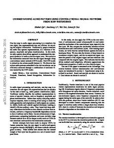
Studying the relationship between input concepts and CNN decisions requires a measure of how well such concepts are recognized by a CNN. We define a concept as being ‘recognized’ if there are a set of late stage convolutional layer nodes that only activate over the the input because of the concept’s presence. Whereas much of the research assumes that these nodes must lie within the same CNN feature map (Bau et al., 2017; Zintgraf et al., 2017), we assert that concept recognition could occur in a distributed way, across many feature maps at a convolutional layer. Past studies have suggested and demonstrated that neural networks learn a representation of input features in a distributed fashion (Carpenter and Grossberg, 1988; Bengio et al., 2003; Hinton, 1986); thus, we do not consider the possibility that input concepts can only be recognized within a single feature map. In the context of scene classification, the recognition of a concept (e.g. an annotated object) would be manifested by a set of (distributed) nodes (across multiple feature maps) that collectively respond to the input pixels representing the concept. If the set of nodes is a “good” recognizer of the concept, they should collectively respond to all pixels representing the concept, and over no pixels not representing the concept. We call a node activated if it takes on a non-zero value under a sigmoid or tanh non-linearity, or is > 0 under a ReLU non-linearity. The deconvolution of a feature map recovers the pixels of an input image causing its nodes to activate (Zeiler and Fergus, 2014; Zeiler et al., 2011; Yosinski et al., 2015). Deconvolutions thus seem like a natural way to identify if input concepts in scenes are represented by a feature map: if the deconvolution of the feature map covers most pixels of a concept, we may consider it as ‘recognized’ by the feature map. However, patterns activating nodes in a feature map are not always consistent from image to image. We illustrate this point in Figure 1 where a feature map, taken from the last convolutional layer of AlexNet trained for object recognition, has its deconvolution computed for different input images. The deconvolution over the first cat image suggests that the feature map recognizes the facial features of a cat, or the texture of a cat’s fur. The deconvolution over the second image, however, recognizes nothing about the cat, and it is unclear if any concept in the third image is recognized by the feature map. Recent approaches for concept recognition find that only a limited number of feature maps consistently recognize a specific concept (Bau et al., 2017). Instead of focusing on concept recognitions localized to a single feature map, Figure 2 summarizes our approach to find and evaluate concepts recognized across multiple feature maps in a convolutional layer. Given a binary segmentation mask of the concept and the deconvolutions of feature maps in the latest stage convolutional layer, a greedy algorithm selects the subset of feature maps that collectively “best" recognize the given concept according to a scoring function. The selected feature maps and a recognition quality score is then returned to the user. The specifics of the recognition scoring and the greedy algorithm are discussed next. 2

Figure 1: Deconvolutions of different cat images over the same feature map

Figure 2: Concept recognition across feature maps

Table 1: Scene classes considered

2.1

Label

Class Name

Num. images

Label

Class Name

Num. images

0 1 2 3 4 5 6 7

bathroom street office building facade airport terminal game room living room hotel room

671 2038 112 228 107 99 697 160

8 9 10 11 12 13 14 15

mountain snowy conference room skyscraper corridor bedroom dining room highway kitchen

132 168 320 110 1389 412 295 652

Recognition scoring

Ideally, the pixel area for a given concept should be covered by the deconvolutions of the selected feature maps as precisely as possible. The score should thus consider the combined coverage of the deconvolutions of the chosen feature maps over and not over the pixels of a concept. Based on this idea, we evaluate how well a set of feature maps Gc recognizes a concept c in an image ξ using a binary segmentation mask Mc (ξ) that denotes the pixel positions of c in ξ. We assume that Mc (ξ) is available in a dataset or can be generated via object segmentation methods (Chen et al., 2016). From the setPof deconvolutions Dc (ξ) = {Di (ξ)} of Gc with respect to ξ and their combined sum Dcsum (ξ) = Dc (ξ), we define Dc (ξ) as the set of the positions of the pixels of Dcsum (ξ) representing node activations across Gc . Then a concept recognition score Sc (Gc , ξ) is defined with a Jaccard like similarity measure similar to Bau et al. (2017): Sc (Gc , ξ) =

2.2

|Mc (ξ) ∩ Dc (ξ)| |Mc (ξ) ∪ Dc (ξ)|

Recognition algorithm

We devise a greedy algorithm to identify the Gc that best recognizes c listed as Algorithm 1. The intuition behind the greedy approach is to find a set of feature maps that recognizes c well, is as small as possible, and is composed of feature maps that minimally ‘overlap’, e.g. recognizes the same parts or qualities of a concept. The latter two criteria capture the idea that a good distributed representation is one where the nodes of each feature map in the set activate over different and significant parts of the 3

concept. Thus, in each greedy iteration, the algorithm searches for the feature map whose addition to Gc would yield the largest improvement in recognition score Sc (Gc , ξ). Large improvements would only be possible if the newly added feature map activates over pixels representing c that no other feature map in Gc activates over. Moreover, this feature map cannot have significant activations over pixels that do not represent c without reducing Sc . Greedy iterations continue until there is no feature map whose inclusion would yield an improvement in score greater than ∆. ∆ = 0.01 is used in the experiments below. Algorithm 1 Concept Localization 1: procedure GREEDY _ SELECTION(G, D, Mc (ξ), ∆) 2: Sc ← 0 . Score of the selected set of feature maps 3: Gc ← {} . Set of selected feature maps 4: while True do 5: tmps ← 0 6: g ← null 7: for k = 1 to |G| do 8: K = Gc ∪P Gk . Add candidate feature map Gk ∈ G to the selected set 9: DK (ξ) = k∈K Dk (ξ) . Sum the deconvolutions Dk of the feature maps in K K

|Mc (ξ)∩D (ξ)| Sc (K, ξ) = |M K c (ξ)∪D (ξ)| if Sc (K, ξ) > tmps then tmps ← Sc (K, ξ) g ← Gk G.remove(g) if tmps − Sc > ∆ then Sc ← tmps Gc .append(g) else return Sc , Gc

10: 11: 12: 13: 14: 15: 16: 17: 18: 19:

3

. Find the new recognition score after adding Gk . Is Gk better than the best candidate found so far?

. Remove the selected feature map from G . Does adding g improve the score by more than ∆? . Add g to the feature map set and repeat

Recognition analysis

We use Algorithm 1 to recognize each concept in each given input image, and study the relationship between its recognition quality and a CNN’s scene classification accuracy. We consider an AlexNet (Krizhevsky et al., 2012) CNN model trained over the Places365 (Zhou et al., 2016) scene dataset and fine tune network weights using ADE20k (Zhou et al., 2017). We only consider the subset of scenes in ADE20k having at least 99 example images. We choose this subset to ensure a sufficient number of examples are available for CNN training and to be able to take representative measurements of the CNN’s ability to classifying a scene correctly. The 16 (out of the 1000+) scenes in ADE20k having at least 99 example images and are listed in Table 11 . 60% of the images from each class are randomly sampled as training data during fine tuning and 40% for testing. The fine-tuned CNN achieves a 74.9% top-1 classification accuracy over the testing images after 30 training epochs, which is higher than the performance of other CNN scene classifiers (Zhou et al., 2016), but we note that we only test over scenes that have an abundance of images in the ADE20K’s training data. We then randomly choose 50 images from each class and compute how well their concepts are recognized by the 256 feature maps in the last convolutional layer of the CNN. This sample of 50 × 16 = 800 images feature 370 distinct concepts. To get a sense of whether a recognition score is relatively “low" or “high", we plot the score distribution across all concepts in the sampled images in Figure 4. We note that the mean recognition score is 0.315 with median 0.284, and the lower and upper quartiles are 0.174 and 0.429 respectively. Figure 3 illustrates the output of Algorithm 1 in a sampled bedroom scene. For the eight concepts annotated in this image, the binary segmentation mask, its label, a visualization of the sum of deconvolutions chosen by our greedy algorithm, and the recognition score are presented. The highest quality recognition is of the bed concept, with a score (0.802) well above the upper quartile of the recognition score distribution across all concepts, a 1

We also omit the ‘misc’ class of ADE20k as it is a catch-all for hard to describe scenes, even though it has over 99 images.

4

700 600 500 400 300 200 100 0 0.0

0.2

0.4 0.6 Recognition Score

0.8

Scene Classification Accuracy

Frequency

Figure 3: Concept recognition results for a given image

1.0

1.0 0.8 0.6 0.4 0.2 0.0 0.20

skyscraper mountain_snowy

airport_terminal 0.25 0.30 0.35 0.40 0.45 Average Concept Recognition

0.50

Figure 5: Recognition quality vs CNN’s accuracy

Figure 4: Recognition score distribution

summed deconvolution that captures texture information about the bed and the shape and patterning of the bed frame, and activates over few pixels that does not represent the bed concept. The chair concept has a lower recognition score (0.287) that happens to be close to the median of the concept recognition score distribution. In this case, the selected feature maps are able to recognize most parts of the chair, including its legs and back, but also happens to activate over some of the straight line and texture patterns of the wall and floor surrounding the chair. The stairs concept has the lowest score (0.225), caused by the feature maps’ inability to activate over all pixels of the concept and also activate across pixels representing the nearby concepts (wall and door). 3.1

Recognition versus performance

We now explore the relationship between concept recognition and CNN performance. For each scene and its sampled images, we compare the average recognition score of concepts within a scene’s images against the CNN’s average classification accuracy of the scene. Figure 5 shows only a weak linear relationship (Pearson’s correlation ρ = 0.187), although there are interesting observations for some scenes. The two scenes with the best classification and recognition scores are skyscraper and mountain_snowy, which are scenes whose images include concepts that are especially emblematic. For example, the mountain concept is captured well across mountain_snowy scenes 5

mountain_snowy (S¯mountain = 0.562 where S¯cs denotes the average recognition of concept c across the sampled scenes of s) and concepts like skyscraper, sky, and building are identified well in skyscraper skyscraper skyscraper skyscraper scenes (S¯sky = 0.532, S¯building = 0.362, S¯skyscraper = 0.407). airport_terminal is a challenging scene for the CNN to identify despite achieving high average concept recognition. This airport_terminal may be due to strong recognitions for concepts like floor and ceiling (S¯floor = 0.585, airport_terminal S¯ceiling = 0.559) that appear in at least 45 of the 50 sampled airport_terminal images, but these concepts are generic and could apply to any kind of indoor scene. Concepts better capturing airport_terminal the notion of an airport terminal are also recognized, e.g., armchair (S¯armchair = 0.555) and airport_terminal shops (S¯shops = 0.548), but they emerge in only one of the sampled images.

3.2

Sparse concepts

The airport_terminal example suggests that there may be particular types of concepts that have stronger or weaker relationships to a CNN’s decisions. We first consider ‘sparse’ concepts, which are concepts appearing in a small number of images within a scene (we quantify this notion with a popularity score in the sequel). Sparse concepts may not appear often enough during training for a CNN to learn to recognize well or to relate with a particular scene. For example, while the CNN is able to recognize the armchair and shops concepts in an airport_terminal well, their infrequency could mean the CNN does not have enough observations to establish a relationship between these concepts and the scene label. Figure 6 explores the prevalence of concepts and how well they are recognized across each of the 16 scene classes. It illustrates that, for every class, there are a majority of concepts that emerge in less than 10 of the 50 images sampled from each scene. Scenes that are relatively uniform in the way they look, for instance skyscraper, mountain_snowy, and street scene, have fewer sparse concepts. Moreover, such scenes tend to have their non-sparse concepts recognized strongly by the CNN (reflected by the steeper slopes of the linear fits in their scatter plots). Scenes that are non-uniform in what they could look like, for example bedroom, hotel_room, and dining_room images that depict different styles and design, tend to exhibit a larger number of sparse concepts. But some of these sparse concepts have high recognition scores (resulting in shallower slopes of the linear fits in their scatter plots), suggesting that the CNN learns to recognize them. This may be because a sparse concept could be observed across a large number of different scenes. For example, although not every bedroom has a chair, one can imagine a chair to appear across a variety of different scenes, giving a CNN enough examples to learn to recognize this concept.

50 40 30 20 10 0 50 40 30 20 10 0

game_room

0.0 0.2 0.4 0.6 0.8 1.0

skyscraper

0.0 0.2 0.4 0.6 0.8 1.0

50 40 30 20 10 0 50 40 30 20 10 0

office

0.0 0.2 0.4 0.6 0.8 1.0

mountain_snowy

0.0 0.2 0.4 0.6 0.8 1.0

50 40 30 20 10 0 50 40 30 20 10 0

building_facade

0.0 0.2 0.4 0.6 0.8 1.0

dining_room

0.0 0.2 0.4 0.6 0.8 1.0

50 40 30 20 10 0 50 40 30 20 10 0

highway

0.0 0.2 0.4 0.6 0.8 1.0

living_room

0.0 0.2 0.4 0.6 0.8 1.0

50 40 30 20 10 0 50 40 30 20 10 0

airport_terminal

0.0 0.2 0.4 0.6 0.8 1.0

bedroom

0.0 0.2 0.4 0.6 0.8 1.0

50 40 30 20 10 0 50 40 30 20 10 0

street

0.0 0.2 0.4 0.6 0.8 1.0

conference_room

0.0 0.2 0.4 0.6 0.8 1.0

50 40 30 20 10 0 50 40 30 20 10 0

kitchen

0.0 0.2 0.4 0.6 0.8 1.0

bathroom

0.0 0.2 0.4 0.6 0.8 1.0

50 40 30 20 10 0 50 40 30 20 10 0

corridor

0.0 0.2 0.4 0.6 0.8 1.0

hotel_room

0.0 0.2 0.4 0.6 0.8 1.0

Figure 6: Average concept recognition (x-axis) vs. number of concept occurrences (y-axis) per scene

The figure and discussion suggest the following hypothesis: the fewer the number of sparse concepts present and the greater the number of well recognized non-sparse concepts appear across the images of a scene, the higher the chance is that the CNN can correctly identify the scene. Moreover, scenes whose images are dominated by a variety of sparse concepts should prove to be more challenging for the CNN to classify. To test this, we plot the slope of the linear fit of each scatter plot from Figure 6 against the CNN’s accuracy for each scene in Figure 7. The moderate linear relationship (Pearson’s ρ = 0.444) suggests that many non-sparse, well recognized concepts are associated with correct CNN decisions, lending support for the hypothesis. 6

250

0.8

200 Frequency

Scene Classification Accuracy

1.0

0.6 0.4

0 0.0

10 15 20 25 30 35 40 45 50 Slope of Concept Recognition vs Popularity

Figure 7: Slope of sparse concept recognition (Figure 6) vs CNN’s accuracy 3.3

100 50

0.2 0.0 5

150

0.2

0.4 0.6 0.8 Uniqueness Score

1.0

Figure 8: Uniqueness score distribution

Unique and misleading concepts

We now investigate non-sparse concepts further. Intuitively, non-sparse concepts may have greater benefit to correct CNN decisions if they appear across a smaller number of different types of scenes. For example, concepts like sand and shell may be present in many beach scenes, are closely associated with the notion of beach, and are unlikely to appear in other types of scenes. Thus, high quality recognition of sand and shell concepts would help a CNN to classify beach scenes correctly. On the other hand, non-sparse concepts emerging across a variety of scenes may be less helpful. For example, since we expect most images of indoor scenes to include concepts like wall, floor, or ceiling, their recognition may not help a CNN differentiate between different indoor scenes. In fact, these recognitions may be of limited help in the best case and could confuse or mislead a CNN to make a wrong classification in the worst case. To explore these ideas, we compute a uniqueness score of a concept that reflects the variety of scenes it appears in. The uniqueness U (c) of a concept c is calculated as: # of scene classes c appears # of scene classes Figure 8 gives the distribution of the uniqueness scores of each concept. It is skewed, with its average uniqueness score at 0.845, and its lower quartile, median, and upper quartile is 0.8125, 0.9375, and 0.9375 respectively. 210 of the 370 concepts appear in only one scene class, although many of these concepts are likely to be sparse. Following the fact that many of the scenes used in our analysis (listed in Table 1) are indoors, concepts with the least unique scores pertain to generic aspects of a room. For example, the concepts having the three lowest uniqueness scores are U (wall) = 0.063, U (floor) = 0.25, and U (door) = U (plant) = U (window) = U (ceiling) = U (picture) = 0.3125. U (c) = 1 −

We hypothesize that the recognition of unique concepts helps a CNN make correct classifications, and that concepts with low uniqueness scores may ‘mislead’ a CNN. We evaluate this hypothesis by comparing the CNN’s classification accuracy to the average recognition score calculated on “unique" concepts and “misleading” concepts respectively. A concept c is labeled as “unique" if its uniqueness score U (c) > α for a uniqueness threshold α. However, we recall from Figure 6 that a number of unique concepts are likely to be ‘sparse’, thus hindering classification accuracy (Figure 7). We thus filter away sparse concepts by defining a popularity score P (c) with respect to some scene by: # of images c appears in a scene class # of images sampled from a scene class and only consider concepts whose P (c) > β for a popularity threshold β. P (c) =

We then compute Pearson’s correlation coefficient ρ between the CNN’s accuracy over each scene class against the average recognition score on “unique” and “misleading” concepts respectively for 7

Figure 9: Heatmap for PCC calculated upon “unique” concept, “misleading” concept, and “synthesized” of unique and misleading concepts using different thresholds.

various values of α and β. Figure 9 presents ρ over a grid of the two thresholds, varying their values in increments of 0.05 between 0 and 1. The left heatmap shows ρ when only unique concepts are considered. Most of the area shows a positive relationship between the unique concepts recognition quality and CNN accuracy. Larger uniqueness and popularity thresholds α and β, making the set of unique concepts even smaller, lead to an even stronger relationship. Note that there is no concept having U (c) ≥ 0.95, causing empty cells in the right most two columns. The middle heatmap only considers misleading concepts. The shaded blue areas indicate a negative relationship between the misleading concepts recognition quality and the model performance. For most valid settings of β, when U (c) < 0.7, there exists a moderate strong negative correlation. This provides some evidence that the recognition of misleading concepts, e.g. those concepts appearing across many different scene types, may be hindering a CNN’s ability to classify scenes correctly. The right heatmap reports ρ using a “synthesized” average concept recognition score, which is defined for each scene class by Ssyn = (Sunique +1.0−Smislead )/2 where Sunique is the average concept recognition score over the unique concepts and Smislead is the same but over misleading concepts. This synthetic score unifies the results from the unique and misleading heatmaps together in search of threshold settings that maximize ρ over unique concepts and minimize ρ over misleading concepts. We find the highest positive correlation of ρ = 0.521 using the synthetic scores when β = 0.4 and α = 0.55. At these thresholds, we find ρ = 0.454; (p = 0.078) over the unique concepts and ρ = −0.528; (p = 0.036) on the misleading concepts. The p-values for these correlation scores, computed over n = 16 classes, indicate a significant negative correlation between misleading concept recognition and CNN’s accuracy, and a moderate positive correlation between unique concept recognition and CNN’s accuracy.

4

Conclusions and future work

This paper investigated the relationship between a CNN’s recognition of input concepts and classification accuracy. A novel approach was developed to quantify how well a concept (specifically, an object in an image) is recognized across the latest convolutional layer of a CNN. Analysis using image object annotations in the ADE20k scene dataset revealed a weak relationship between the average recognition of image concepts in a scene and classification accuracy. We found evidence to suggest that the relationship is hindered by recognized concepts that are “sparse”, or appear in a small number of images of a scene and by “misleading” concepts that appear in many images across many different scenes. Recognizing “unique” concepts, which appear often but in a limited set of scenes, is moderately positively correlated with the CNN’s classification accuracy. For future work, we will analyze which feature maps are necessary to accurately model each object in the scene. The effects of “unique”, “misleading”, and “sparse” concepts will be explored in more detail. In particular, we will investigate common misclassifications for a scene and seek explanations by the recognized concepts that are (not) common between them. We will study the effect of “sparse” concepts on CNN classification via their occlusion in an image. We will also explore the mechanics of how concept recognitions impact downstream network activations leading to a decision and devise a measure of the importance of concept recognition to CNN decision making. 8

References Bach, S., Binder, A., Montavon, G., Klauschen, F., Müller, K.-R., and Samek, W. (2015). On pixel-wise explanations for non-linear classifier decisions by layer-wise relevance propagation. PloS one, 10(7), e0130140. Bau, D., Zhou, B., Khosla, A., Oliva, A., and Torralba, A. (2017). Network dissection: Quantifying interpretability of deep visual representations. arXiv preprint arXiv:1704.05796. Bengio, Y., Ducharme, R., Vincent, P., and Jauvin, C. (2003). A neural probabilistic language model. Journal of machine learning research, 3(Feb), 1137–1155. Carpenter, G. A. and Grossberg, S. (1988). The art of adaptive pattern recognition by a self-organizing neural network. Computer, 21(3), 77–88. Chen, L.-C., Papandreou, G., Kokkinos, I., Murphy, K., and Yuille, A. L. (2016). Deeplab: Semantic image segmentation with deep convolutional nets, atrous convolution, and fully connected crfs. arXiv preprint arXiv:1606.00915. Doran, D., Schulz, S., and Besold, T. R. (2017). What does explainable AI really mean? A new conceptualization of perspectives. arXiv preprint arXiv:1710.00794. Dosovitskiy, A. and Brox, T. (2016). Inverting visual representations with convolutional networks. In Proc. of IEEE Conference on Computer Vision and Pattern Recognition, pages 4829–4837. Girshick, R., Donahue, J., Darrell, T., and Malik, J. (2014). Rich feature hierarchies for accurate object detection and semantic segmentation. In Proc. of IEEE Conference on Computer Vision and Pattern Recognition, pages 580–587. Hinton, G. E. (1986). Learning distributed representations of concepts. In Proc. of the Annual Conference of the Cognitive Science Society, volume 1, page 12. Amherst, MA. Krizhevsky, A., Sutskever, I., and Hinton, G. E. (2012). Imagenet classification with deep convolutional neural networks. In Advances in Neural Information Processing Systems, pages 1097–1105. LeCun, Y., Bottou, L., Bengio, Y., and Haffner, P. (1998). Gradient-based learning applied to document recognition. Proceedings of the IEEE, 86(11), 2278–2324. Lipton, Z. C. (2016). The mythos of model interpretability. arXiv preprint arXiv:1606.03490. Mahendran, A. and Vedaldi, A. (2015). Understanding deep image representations by inverting them. In Proc. of IEEE Conference on Computer Vision and Pattern Recognition, pages 5188–5196. Montavon, G., Lapuschkin, S., Binder, A., Samek, W., and Müller, K.-R. (2017). Explaining nonlinear classification decisions with deep taylor decomposition. Pattern Recognition, 65, 211–222. Ren, S., He, K., Girshick, R., and Sun, J. (2015). Faster r-cnn: Towards real-time object detection with region proposal networks. In Advances in Neural Information Processing Systems, pages 91–99. Selvaraju, R. R., Cogswell, M., Das, A., Vedantam, R., Parikh, D., and Batra, D. (2016). Gradcam: Visual explanations from deep networks via gradient-based localization. arXiv preprint arXiv:1610.02391. Simonyan, K. and Zisserman, A. (2014). Very deep convolutional networks for large-scale image recognition. arXiv preprint arXiv:1409.1556. Sun, Y., Chen, Y., Wang, X., and Tang, X. (2014). Deep learning face representation by joint identification-verification. In Advances in Neural Information Processing Systems, pages 1988– 1996. Yosinski, J., Clune, J., Nguyen, A., Fuchs, T., and Lipson, H. (2015). Understanding neural networks through deep visualization. arXiv preprint arXiv:1506.06579. Zeiler, M. D. and Fergus, R. (2014). Visualizing and understanding convolutional networks. In European Conference on Computer Vision, pages 818–833. Springer. 9

Zeiler, M. D., Krishnan, D., Taylor, G. W., and Fergus, R. (2010). Deconvolutional networks. In Proc. of IEEE Computer Vision and Pattern Recognition Conference, pages 2528–2535. IEEE. Zeiler, M. D., Taylor, G. W., and Fergus, R. (2011). Adaptive deconvolutional networks for mid and high level feature learning. In Proc. of IEEE Conference on Computer Vision, pages 2018–2025. IEEE. Zhang, J., Lin, Z., Brandt, J., Shen, X., and Sclaroff, S. (2016). Top-down neural attention by excitation backprop. In European Conference on Computer Vision, pages 543–559. Springer. Zhou, B., Khosla, A., Lapedriza, A., Torralba, A., and Oliva, A. (2016). Places: An image database for deep scene understanding. arXiv preprint arXiv:1610.02055. Zhou, B., Zhao, H., Puig, X., Fidler, S., Barriuso, A., and Torralba, A. (2017). Scene parsing through ade20k dataset. In Proc. of IEEE Conference on Computer Vision and Pattern Recognition. Zintgraf, L. M., Cohen, T. S., Adel, T., and Welling, M. (2017). Visualizing deep neural network decisions: Prediction difference analysis. arXiv preprint arXiv:1702.04595.

10