compression techniques. In this paper, we design and implement a novel database compression technique based on vector quantization (VQ). VQ is a data com ...
Relational Database Compression Using Augmented Vector Quantization*t WEE K. NG
CHINYA V.
~VISHANKAR
Department of Electrical Engineering and Computer Science The University of Michigan, Ann Arbor, MI 48109-2122 E-mail: {wkn,ravi}Oeecs.umich.edu
Abstract
sion differs from data compression in general. Conventional data compression is usually performed at the granularity of entire data objects. Access to random portions of the compressed data objects is impossible without decompressing the entire object. Clearly, this is not practical for database systems. What is required is a technique that not only compresses data well, but also supports standard database operations. In this paper, we design a novel database compression technique that has the following characteristics: (1) it is lossless, (2) it compresses/decompresses locally, thus permitting localized access to compressed data, and (3) it supports standard database operations as described above. The technique is based on the concept of Vector Quantization (VQ). Conventional VQ is a lossy data compression technique with wide applicability in speech and image coding [3, 51. We propose a lossless version called Augmented Vector Quantization (AVQ) that is appropriate for database compression. We have also restricted our attention to relational databases as they are very widely used. This paper is organized as follows. Section 2 provides background material for conventional lossy vector quantization. We also discuss how VQ may be adapted for database compression. In Section 3, we describe issues in the practical implementation of AVQ. Section 4 illustrates how AVQ supports standard database operations. We evaluate the performance of AVQ in Section 5 . Finally, the last section concludes the paper.
Data compression is one way t o alleviate the 1/0 bottleneck problem faced by I/O-intensive applications such as databases. However, this approach is not widely used because of the lack of suitable database compression techniques. In this paper, we design and implement a novel database compression technique based on vector quantization (VQ). VQ is a data compression technique with wide applicability in speech and image coding [3, 51, but it is not directly suitable for databases because it is lossy. We show how one may use a lossless version of vector quantization t o reduce database space storage requirements and improve disk I / O bandwidth.
1
Introduction
Processor speed, memory speed, and memory size have grown exponentially over the past few years. However, disk speeds have improved at a far slower rate. As a result, many applications such as database systems are now limited by the speed of their disks rather than the power of their CPUs [l]. As improvements in processor and memory speeds continue to outpace improvements in disk speeds, the severity of the 1/0 limitation will only increase. One way to alleviate this problem is through database compression [2, lo], which will not only reduce the space requirements, but also increase the effective 1/0 bandwidth since more data is transferred in compressed form. However, this approach has not been widely adopted. One reason is the lack of suitable database compression techniques. Database compres-
2 2.1
*This work was supported in part by the Consortium for International Earth Science Information Networking. 'The material contained in this paper may be covered by a pending patent application [11].
Conventional vector quantization
Multidimensional vector quantization (or VQ) is a technique for lossy encoding of n-dimensional vectors.
540
1063-6382/95 $4.00 0 1995 IEEE
Augmented Vector Quantization
The set Y of output vectors is also called the codebook. Given a set of input vectors, the design of optimal codebooks has been extensively studied by Linde, Buzo and Gray [9]. They have proposed an algorithm that determines the optimal codebook via iterative refinements. This method is inefficient as it requires a non-deterministic number of iterations. As we shall see, our adaptation of VQ (AVQ) has a definite advantage over their algorithm: It computes the codebook in constant time. Another issue that determines the performance of VQ is the structure of the codebook. During decoding, the codebook should be structured as to permit efficient searching of codewords. For large codebooks, this search process can become computationally intensive. Many structures have been proposed to reduce the search time [5]. In this respect, AV& has another advantage: No searching is required.
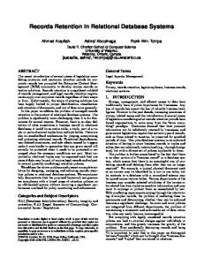
Figure 2.1: Block diagram of a vector quantizer.
Conventional VQ operates as follows. Let X be an (possibly infinite) input set of n-dimensional vectors. First, a fixed and finite set Y of n-dimensional out> IYI. Each zi E X put vectors is selected, with is mapped into a gj E Y which approximates it according to some suitable criterion, and yj is output in place of zi. Since the set Y of output vectors is finite, a codeword j can be used to identify each output vector gj representing an original input vector zi. Compression is achieved because the size of each codeword j is smaller than that of the corresponding zi. During decoding, the codeword j is simply replaced by the output vector yj, approximately reconstructing the original input vector zi. The coding/decoding process is illustrated in Figure 2.1. A brief formalization is given below: A vector quantizer Q : W" -+ Y is a mapping of n-dimensional Euclidean space W" into a finite subset Y of W", where n > 1, Y = {y1,y2,.. .,y,}. Each yi E W" is an output vector. Y induces a partition of W": RI, Rz,. . . ,R,,,where R, = Q-'(yj) = {z E W" I Q(z) = vi}. Thus, UzlR, = W" and R, n R, = q5 for all i # j . The quantizer is uniquely defined by the output set Y and the corresponding partition {R,}. The quantizer can also be seen as a combination of two functions: a coder and a decoder. The coder C is a mapping of W" into the index or codeword set J = { 1 , 2 , . . .,m} and the decoder D is a mapping of J into the output set Y. A distortion measure d ( z , 12) represents the penalty associated with reproducing vectors z by 12 = Q(z). A commonly used measure is the square error between z and z defined as follows:
1x1
2.2
A relational database is a natural candidate for the application of VQ. A relation is a table of n-tuples, each of which is a vector, or a point in n-dimensional space. We will use the terms iuple and vector interchangeably. A direct application of VQ to encode a relation would be to find a set of representative tuples, and replace each tuple in the relation with a codeword or index that indicates the representative tuple that is closest to it. Unfortunately, this method of coding is lossy; the original tuples are no longer completely recoverable. Thus, a new design is needed. We propose Augmented Vector Quantization (AVQ), a lossless database compression technique based on VQ. Instead of replacing each tuple in a relation only by its codeword as VQ does, we also include the difference between the tuple and its representative tuple. The method is formally defined below. But first, we need some preliminaries in relational database terminology. A relation scheme 'R = ((AI, Az, . . .,An)) is the Cartesian product of the set of attributes Ai, i.e., 72 = A1 x A2 x . . . x A,, . It corresponds to the ndimensional space W" as defined in the previous section except that the size of each dimension IAjl, may not be the same, and the value a E Ai within each dimension or domain is non-negative. A relation R is a subset of 'R and corresponds to the set of input vectors to be coded. A tuple t E R is an n-dimensional vector. All points in 'R may be totally ordered via an orderingrule. Let NR = { 0 , 1 , . . ., 117211-1) be a s e t of integers that correspond to 'R, where ll'Rll = E:='=lAil , is
n
- ii)'
d ( z ,i)=
Database compression
(2.1)
i=l
The optimal quantizer Q is the one that minimizes d ( z , 5 ) for all input vectors z (31.
541
the size of the 'R space. Define a function 'p : 72 -+ JVR as follows:
Theorem 2.1 (Lossless property) AVQ is lossless. Proof: During the coding process, a tuple t is quantized into a codeword C ( t ) and a difference d ( t , Q ( t ) ) . By definition of the difference measure (Equation 2.6),
for all (al, 0 2 , . . ., a,)l E 'R. The inverse of fined as: 'p-'(e) = ( a i , a k ,..., a;)
'p
d(t,Q(t)) = d Q ( t ) ) - ~ ( t ) d t ) = d Q ( t ) )- d ( t , U t ) )
is de-
assuming t 4 Q ( t ) . During decoding, C ( t ) indicates that Q ( t ) is the output vector. By subtracting the difference from 'p(Q(t)),one obtains 'p(t). From the definition of 'p (Equations 2.2 and 2.3), 'p is a bijection. Thus, 'p(t)is uniquely mapped back to the tuple t which is then completely recovered. The same arguI ment holds when Q ( t ) 4 t .
(2.3)
for all e ENx and i = 1 , 2,..., n - 1,
n
3 where a; = e and a; = 'p is a n-dimensional to 1-dimensional mapping that maps a tuple t E 'R uniquely into its ordinal position in the 'R space. Given two tuples t i , t j E R, we may define a total order based on 'p, denoted by ti 4 t j , such that t i precedes t j if and only if V ( t i ) < ' p ( t j ) . With these preliminaries, the difference between any two tuple t i , t j may be defined as: d ( t i ,t j ) =
' p ( t j ) - 'p(ti) ' p ( t i )- ' p ( t j )
if ti 4 t j otherwise
Implementation of AVQ
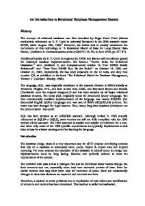
We now see how AVQ may be adapted for database compression. In particular, we are interested in how a relation is encoded and allocated physically to disk blocks. Sections 3.1-3.4 illustrate the steps in the process of transforming a relation into a set of losslessly quantized tuples. Throughout this section and the rest of the paper, we use the relation described in Example 3.1 to illustrate the concepts involved. Example 3.1 Table (a) in Figure 2.2 shows a relation R with five attribute domains A I ,Az, As, Aq, A5 denoting the department, j o b W e , years in company, hours worked per week, and employee number respectively. The size of each domain, i.e., the number of attribute values, is 8,16,64,64,64 respectively. Table (b) shows the same relation, except that the attribute values have all been encoded to numbers. Attribute encoding is discussed briefly below. The relation in the figure has been partitioned into blocks. I Each block is coded/decoded individually.
(2.6)
AVQ is defined by the quantizer QL as follows: Definition 2.1 (AVQ) . Given a vector quantizer Q : 'R + Z+, QL : 'R + Z+x n/7P is a lossless mapping that encodes a tuple t E R by the pair ( C ( t )d, ( t , Q ( t ) ) ) , where C is the coder that produces the codeword (or index into the codebook) denoting
Q(t)Let p[z] denote the minimum number of bits in the binary representation of number z. If p[C(ti)] P [ d ( t i ,& ( t i ) ] < p [ t i ] , then compression is achieved. The compression efficiency of AVQ depends on the choice of the codebook. If the codebook is properly designed, the average difference between a tuple and its representative tuple will be small enough that it takes fewer bits to encode than the original tuple. We have so far claimed that AVQ is lossless. This is shown in the following theorem:
+
3.1
Attribute encoding
A variety of attribute domain types are encountered in practice. Attributes such as social security numbers or zip codes are numeric, while those such as names and addresses are alphanumeric, occurring in the form of ASCII characters. The first preprocessing step in AVQ encodes each attribute value to a number. For discrete finite domains where all the attribute values are known in advance, each attribute value is mapped to its ordinal position in the domain. For other domain types, more work is needed. For alphanumeric
'A tuple is generally enclosed in angle brackets. When used as an argument of a function, the angle brackets are omitted when no confusion arises.
542
11 A2 A3 A4 A5 vroduction marketing management marketing management vroduction vwduction vroduction marketing vroduction marketing production production marketing marketing personnel production marketing marketing production marketing marketing production personnel production personnel production marketing marketing production marketing marketing personnel production production production management production production marketing production marketing marketing marketing marketing marketing production personnel production marketing
part-time director workerl worker2 supervisor secretary secretary workerl worker2 ezecutive part-time secretary manager manager worker2 supewisor part-time part-time manager manager secretary manager manager manager workerl worker2 worker2 workerl supervinor manager worker2 part-time supervisor part-time superviaor manager workerl part-time supervisor supervisor worker2 manager manager supervisor ezecutive manager worker2 secretarq worker2 worker2
24 12 29 30 27 23 34 32 39 31 19 28 32 38 26 33 34 25 41 32 39 50 31 26 34 45 39 40 30 24 33 32 19 27 32 36 26 26 35 39 35 32 31 35 55 32 37 24 30 39
32 31 21 42 27 25 28 37 37 25 21 22 34 34 32 22 28 27 28 25 29 26 33 32 26 16 37 27 44 30 32 42 31 26 30 39 20 27 25 33 28 24 24 19 23 27 31 26 32 31
3 4 2 4 2 3 3 3 4 3 4 3 3 4
00 01 02 03 04 05 06
07 08 09
10 11 12 13 14 15 16 17 18 19 20 21 22 23 24 25 26 27 28 29 30 31 32 33 34 35 36 37 38 39 40 41 42 43 44 45 46 47 48 49
I
09 24 32 00
2 2 2 3 3 3 3 3 3 09 3 10 3 11 3 12 3 13 3 3 5 15 3 4 141 3 16 3 4 17 3 4 18 3 3 19 3 4 20 3 4 21 3 3 22 3 5 23 3 3 24 4 5 25 4 3 26 4 4 27 4 4 28 4 4 4 4 4 4 3 10 32 30 34 4 3 08 36 39 35 4 2 06 26 20 36 4 3 09 26 27 37 4 3 10 35 25 38 4 4 10 39 33 39 4 3 07 35 28 40 4 4 08 32 24 41 4 4 08 31 24 42 4 4 10 35 19 43 4 4 04 55 23 44 4 4 08 32 27 45 5 3 07 37 31 46 5 5 05 24 26 47 5 3 07 30 32 48 5 4 07 39 31 49 5 12 12 06 29 07 30 10 27 05 23 05 34 06 32 07 39 04 31 09 19 05 28 08 32 08 38 07 26 10 33 09 34 09 25 08 41 08 32 05 39 08 50 08 31 08 26 06 34 07 45 07 39 06 40 10 30
31 21 42 27 25 28 37 37 25 21 22 34 34 32 22 28 27 28 25 29 26 33 32 26 16 37 27 44
01 02 03 04 05 06 07 08
NR
06 26 20 36 10069284 06 29 21 02 10081602 10 27 27 04 11122372 04 31 25 09 13760073
05 23 25 05 05 28 22 11 05 34 28 06 06 32 37 07 06 34 26 24 07 30 32 48 07 35 28 40 07 37 31 46 07 39 37 26 08 24 30 29 08 31 33 22 08 32 25 19 08 32 34 12 08 36 39 35 09 24 32 00 09 26 27 37 09 27 26 33 09 34 28 16 10 32 30 34 10 35 25 38 04 55 23 44 05 39 29 20 06 40 27 27 07 26 32 14 07 30 42 03 07 33 32 30 07 39 31 49 07 39 37 08 08 31 24 42 08 32 24 41 08 32 27 45 08 38 34 13 08 41 28 18 08 50 26 21 09 19 21 10 09 25 27 17 09 32 42 31 10 30 44 28 10 35 19 43 10 39 33 39 12 12 31 01 05 24 26 47 07 45 16 25 08 26 32 23 10 19 31 32 10 33 22 15 Table (c'
13989445 14009739 14034694 14289223 14296728 14542896 14563112 14571502 14580058 14780317 14809174 14812755 14813324 14830051 15042560 15050469 15054497 15083280 15337378 15349350 18052588 18249556 18515675 18720782 18737795 18749470 18774001 18774344 19002922 19007017 19007213 19032205 19044114 19080853 19215690 19240657 19270303 19524380 19543275 19560551 19974081 22382255 22991897 23177239 23672800 23729551
Ai A2 A3 A4 A5
NR
0 00 03 00 30 0 03 62 06 02 2 10 27 27 04 0 10 03 62 05 0 00 55 63 60 0 00 06 05 59 0 00 62 09 01 3 06 32 37 07 0 00 01 53 17 0 00 60 06 24 0 00 02 03 06 0 00 02 05 44 3 07 39 37 26 0 00 48 57 03 0 00 07 02 57 0 00 00 08 57 0 00 04 05 23 3 08 36 39 35 0 00 51 56 29 0 00 01 59 37 0 00 07 01 47 0 00 62 02 18 3 10 32 30 34 0 00 02 59 04 0 10 19 62 06 0 01 00 62 07 0 00 50 04 51 4 07 26 32 14 0 00 04 09 53 0 00 02 54 27 0 00 00 05 23 0 00 55 51 34 4 08 31 24 42 000006363 0 00 00 03 04 0 00 02 58 05 0 00 08 62 03 4 08 50 26 21 0 00 32 58 53 0 00 06 06 07 0 00 62 01 61 0 00 04 39 15 4 10 35 19 43 0 00 04 13 60 0 01 36 61 26
12318 1040770 11122372 2637701 229372 24955 254529 14289223 7505 246168 8390 8556 14580058 200259 28857 569 16727 14830051 212509 7909 28783 254098 15337378 11972 2703238 266119 205107 18720782 17013 11675 343 228578 19002922 4095 196 11909 36739 19080853 134837 24967 254077 18895 19543275 17276 413530
Figure 2.2: A relation R and its transformation after domain mapping. Table (a) is the original relation and Table (b) is the resulting table after mapping every attribute value t o an integer. Table (c) shows the relation after tuple reordering. Table (d) shows the LLVQ coding within blocks.
543
strings, we may construct a table containing the set of these strings and replace each attribute by an index into the table [SI. Other schemes may be used [7, 131. Observe that this step by itelf achieves compression because an attribute value that consists of a long string of ASCII characters is mapped to a short number.
3.2
3 3 3 3 3 [I
17296
09 26 27 37 15050469 A2 A;Ie::I Na
0 00 53 52 02
A2 -4;.&=51
220418
NR
1
2 51 56 29 2 01 59 37
Table
(c)
Table (d)
Figure 3.3: Stages in coding a block o f tuples. Table (a) shows a block o f tuples and Table (b) shows the block after LLVQ coding. Table (c) shows the block after subtraction and Table (d) shows the block after run-length coding.
Block partitioning
A problem with conventional data compression techniques is that coding and decoding is performed at the granularity of data objects. In order to restrict the scope of coding/decoding, we partition the re-ordered relation into p disjoint subsets of tuples, B1,B2,.. . ,Bp. We have chosen the size of a memory page or disk sector as the partition size as it is the unit of 1/0 transfer. That is, the number of bytes occupied by the set of tuples in a partition is no more than the size,of a disk block. When a tuple is required, the block where it resides is transferred from disk to main memory. If tuples in the block are coded, then decoding need only be performed on the block. Hence, coding and decoding is localized.
3.4
0 00 04 14 16
08 32 34 12 14813324 0 00 04 05 23 16727 08 36 39 35 14830051 3 08 36 39 35 14830051 09 24 32 00 15042560 0 00 51 56 29 212509
Tuple re-ordering
The next preprocessing step is to re-order the tuples by an ordering rule, such as that defined by 'p (Equation 2.2). Table (c) in Figure 2.2 shows the tuples ordered lexicographically by 'p. The importance of this step will soon be clear.
3.3
08 32 25 19 14812755
Example 3.2 Consider the fourth block of Table (c) in Figure 2.2 as shown in Table (a) of Figure 3.3. Column NR shows the result of mapping each tuple in column 1 into a number by 'p. Taking (3,08,36,39,35) as the representative tuple, the other tuples are replaced by their differences. For instance, (3,08,32,34,12), which is lexicographically before the representative tuple, is replaced by ( O , O O , 04,05,23) since 'p(O,OO, 04,05,23) = ~ ( 3 , 0 8 , 3 6 , 3 9 , 3 5-) 9(3,08,32,34,12) = 14830051 14813324 = 16727. I The differences may be reduced further by making additional subtractions. For a tuple that is lexicographically after the representative tuple, additional difference may be obtained by subtracting the preceding tuple~fromitself. For a tuple that is lexicographically before the representative tuple, additional difference is obtained by subtracting itself from the succeeding tuple. The following example from Table (c) illustrates:
Block coding
A block Bk now consists of a set of tuples ordered lexicographically, i.e., & = ( t t , l , t t , f , . . . , t k , " ) , t k , i E R, with t k , i < t k , j for i < j . The middle tuple in each block & is chosen as the representative tuple i k of the block. Thus, every tuple t t , j E Bt is mapped to it. Why is the middle tuple representative? After tuple reordering and block partitioning, tuples in a block form a cluster. The median of this cluster is a tuple i such that the total distortion ( ' p ( t k , i ) - 'p(9l is minimized. With the representative tuple known, all the other tuples are AVQ coded into pairs as per Definition 2.1. However, the index component is redundant since the representative tuple is known and unique for all tuples in the block. Hence, we need only replace each tuple by its difference from i k .
cy='=,
Example 3.3 Consider tuple (0, 00,04,14,16) in Table (b). It is replaced by (0,00,00,08,57) obtained as fOllOWS: ~p(0,00,00,08,57)= p(O,OO, 04,14,16) 'p(0, 00,04,05,23) = 17296 - 16727 = 569. This optimization produces Table (c). I Notice the run of leading zeros in each tuple of Table (c). These zeros arise because the differences we are storing require fewer bits than do the original tuples. By coding these runs using run-length coding
544
[4], we obtain Table (d). The runs are replaced by a count of the number of zeros. Coding is complete when these tuples are concatenated as a single stream of data, with the representative tuple being placed in the front. The stream for the block in the example is:
block1
a.1 U . L I . L I . u4>
< 2,03,00,30>
30836393530857204052325156292015937
In AVQ, each block is coded using the above sequence of steps into a stream of bytes. If m is the size of a tuple, the stream may be parsed as follows: The first m bytes give the representative tuple. The next byte is a count field, and gives the number of leading zeros in bytes for the next tuple in the block. If this value is r, then the next m - r bytes are read to get the second tuple. The next byte that follows is again a count field, and the process repeats until all the differences are read. Note that the first and second halves of these differences represent tuples which are lexicographically smaller and larger than the representative tuples respectively. We end with a note regarding the amount of unused space left in the block after coding the tuples: The number of tuples allocated to a block before coding must be suitably k e d so as to minimize this space. The entire relation R after AVQ is shown in Table (d) of Figure 2.2.
4
DB Structure and Operations
< <
2,62,09,01> 2,01,53,11> 2,60,06,24>
2,51,56,29> 2,01,59,37>
< I
I
I
\
I
T
block6
2,04,09,53> 2,02,54,27> block7 ( 4 I un. 31, L4,4 < 3,05,23> c 2,55.51,34>
In this section, we consider how access mechanisms may be constructed on the coded tuples, and how the tuples may be retrieved and modified.
block8 2.32.58.53>
I
block9
< <
2,04,39,15> 2,04,13,60>
\
block10 -,U
,
I
I
j>
c 2,45,15,62> < 2,13,54,47> Level 2
Level 1
Level 0
Data blocks
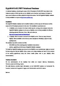
Figure 4.4: Primary index. T h e search key is an entire tuple. Each block begins with a representative tuple. All tuples following the representative tuple are difference tuples, in which the first value is the count of leading zeros.
545
zgI I
Aa A3 A4 A51 Nx / / A I Aa A3 A4 A s / 3 08 32 25 19 14812755 0 00 00 08 57 3 08 32 34 12 14813324 0 00 04 05 23 16727
1-41
Unquantized block buc
3
m 02:01 03:OK 04:01 05:Ol
17:08 18:08 19:04 20:06 21 :08 22:03 23:lO 24:02
[I
27:06 28:09 29:03 30:06 31: 09 32:lO
36:Ol
3
44:05 45:0 1 46: 03 47: 10
3 3 3 3
40:03
-
Figure 4.5: Secondary index for As. T h e buckets provide a level of indirection between attributes of A5 and the tuples of R. Each bucket contains a set o f pair ( a : b) where a is the attribute value and b indicates the data block where the tuple whose A5 = a resides.
I[
A2 A3 A4 -451 Na 3 08 32 25 19 14812755 08 32 25 64 14812800 08 32 34 12 14813324
08 36 39 35 14830051 09 24 32 00 15042560 09 26 27 37 15050469 Unquantized block
Quantized block
0 0 0 3 0 0
A2 A3 A4 -451 00 00 00 45 00 00 08 12
2
1
00 04 05 23
16727 08 36 39 35 14830051 00 51 56 29 212509 00 01 59 37 7909 Quantized block
Figure 4.6: Tuple insertion in a LLVQ coded block. T h e two tables above are before insertion, while the two tables below are after insertion. T h e new tuple is shown in italic.
where the tuple resides. This block is now transferred the data block, and changes made within the block. to main memory and decompressed. Thus, traversing Tuple modification may simply be defined as a comthe index is the same except that key comparison rebination of tuple insertion and deletion. quires measuring the difference between the key and the target tuple. In summary, standard database operations remain the same even when the database is AVQ coded. The When tuples are to be retrieved given certain atonly difference is that the search key of the primary tribute values only, secondary indices are needed. Figindex of a AVQ coded relation is an entire tuple. All ure 4.5 shows an order-3 B+ tree index where A5 is the search key. Since the relation is physically clustered other indices are non-clustering and secondary, as in via cp, the index is non-clustering and secondary. This standard databases. A further advantage of an AVQexplains the extra level of indirection provided by the coded database is that the storage requirements for buckets in the figure. Each bucket contains a pair the indices will be reduced because the number of data ( a : b) where b indicates the data block whose tuples blocks for storing the database has been reduced by ). have A5 = a. Suppose we wish to execute U A ~ = ~ ~ ( Rcompression. Although we have illustrated the use of tree indices as the access mechanisms, we do not Traversing the index points t o bucket 5, where the tuple resides. preclude the use of other methods, such as hashing.
4.2
Tuple insertion and deletion
How are tuple insertions and deletions supported in a compressed database? Suppose we wish to insert tuple (3,08,32,25,64). Using the primary index, we identify data block 4 as the set of insertion. The tuple is found to lie lexicographically between the first and second tuple in the block. Thus, the differences from the representative tuple must be recomputed. Figure 4.6 shows the result of tuple insertion. Notice that differences are re-computed only for tuples before the representative tuple, and that the changes are confined to the affected block. For tuple deletion, the primary index is similarly used to locate
5
Performance Evaluation
The goals of database compression are both to reduce space requirements as well as to improve the response time of 1/0intensive queries. In this section, we look into the compression ratio (Section 5.1), average compression/decompression time (Section 5.2) and the effects of database compression on query response time (Section 5.3). We shall see how both the reduction of 1/0 and the improvement in 1/0 bandwidth contribute to the improvement in query response time.
546
tuples. Considering the domain mapping already performed, the actual efficiency is higher.
Testnumber 1 2 3 4 Dataskew Yes Yes No No Domainvariance Small Large Small Large
0
No. of tuples I Test 1 I Test 2 ITest 3 I Test 4 104
105 lo6
I 73.0%165.6% I
73.0% I 65.6% 70.6% 66.7% 70.6% 66.7% 71.4% 65.5% 71.4% 65.5%
Figure 5.7: Compression efficiency. T h e figures in Table (b) are obtained via the formula: lOO(1 - a/b)% where b and a are the size of the database before and
0
Homogeneity in domain sizes affects the compression efficiency. More homogeneity increases efficiency, as the figures in Tests 1and 3 are relatively higher than the figures in Tests 2 and 4. Therefore, a relation whose range of actual attribute values in each domain does not differ much yields better compressibility. Data skew does not Seem to affect compression efficiency as the figures in Tests 1 and 2 are the same as the figures in Tests 3 and 4.
after coding respectively.
5.2 5.1
Compression efficiency
We measure the average time taken to encode a set of tuples such that the size of the coded tuples can be allocated to a disk block with minimal unused space left in the block. We also measure the time to decode the block. The relation characteristics are as follows: We use a relation with 16 attributes of varying domain sizes. After domain mapping, each tuple is 38 bytes and there are lo5 tuples in the relation. The block size is taken to be 8192 bytes. The measurements are made for each of the three techniques. For each of them, we perform the coding 100 times, and then the decoding 100 times. The average times for each operation are then computed. Before coding, the required number of tuples is first loaded into main memory so as to offset any 1/0 time. The measurements are taken when the coding routine is the only user-level process executing in the system. The results are shown in rows 1 and 2 in Figure 5.9. It is to be noted that the block after decoding is a collection of tuples whose attribute values are integers. Another level of decoding is needed to map the values back to their alphanumeric values originally. We have omitted the measurement of this because the decoding overhead is approximately the same for all techniques.
In order to compare the compression performance of each of the variants, we only have to compare the size of a relation before and after compression. However, what constitutes a typical relation? In order to ensure a fair evaluation, we generated relations of various sizes and characteristics. They differed in: (1) relation size (i.e., the number of tuples), (2) variance in attribute domain size, and (3) attribute value skew. When the differences in domain sizes were no more than 10% of the average domain size, we took the domain size variance to be low. When the differences were more than loo%, we took the variance to be high. The distribution of values within a domain was taken to be skewed when 60% of the values were drawn from 40% of the domain. When no skew existed, values were drawn uniformly from the domain. The number of attribute domains of all relations were fixed at 15. We measured the number of disk blocks required by a relation under these variants. With these parameter variations, four sets of simulations were performed. The domain variance and attribute value skew parameters give a total of four combinations of relation characteristics: small variance and no data skew, large variance and no data skew, small variance and data skew, large variance and data skew. The relation size are varied in each of these combinations. These combinations are tabulated in Table (a) in Figure 5.7. The results of the simulations are shown in Figure 5.7. The following observations may be made: 0
Coding/decoding time overhead
5.3
Response time
In order to perform any measurement, we need the notion of a typical query. This is difficult because as there are many possibilities. Each query is specified by (1) the number of attributes involved, (2) the logical operators on these attributes, (3) the arithmetic operations to be performed, etc. To simplify things, we make the following assumptions:
The data size is greatly reduced for a compressed relation. This is clear from the high compression efficiencies shown in Table (b). Recall that the relation being compressed is a table of numerical
547
Queries are I/O-intensive, so that they are directly affected by the 1/0 bottleneck problem.
Attribute No.1 1 I 2 I 3 I 4 I 5 I 6 I 7 No codinn I33118911891189118411051183
All queries reduce to a set of tuple access operations. The time €or these operations form the bulk of the overall query response time. Thus, it directly affects query performance. Figure 5.8: Estimating N , the number of blocks ac-
We consider query of the form U a s A r < b ( R ) , where Ak is any non-primary key attribute and a, b E A I . . By varying a and b suitably, the number of tuples accessed can be made larger, and thus more I/O-intensive. The tuple access operation is the only one in the query and directly determines the cost of the query. C1, the total time taken to bring in the relevant disk blocks into main memory for further processing in the above query is given by the following expression:
Cl = I
+ N(t1 +tz)
cessed.
+
20 ms + 8 ms (8192 b/3 Mb) ms + 2 ms M 30 ms As the relation characteristics are the same as that of Section 5.2, the average time for single block decompression, t z , is already measured in that section. The estimations for t 3 are given in row 4 in Figure 5.9.
(5.7)
5.3.3
where I is the index search time, N is the number of disk blocks accessed, t l is the time to read a block, and t2 is the decompression time per block. When the database is not compressed, the corresponding cost Cz, is: c 2=I N(t1 t3) (5.8) where t3 is the time to read and extract a block into a set of tuples. This time is included in t2, since the decompression yields a set of tuples.
+
5.3.1
We measure N via simulations. The relation R used has the same characteristics as that of Section 5.2. The selection query u a s A h s b ( R ) has three parameters: k,a, 6. Figure 5.8 gives the number of blocks accessed when executing the query for each of the attributes of a tuple, i.e., k = 1 , 2 , . . ., 15, and where a = 0.5 x IAkI. Observe that only one block is accessed when k = 15 because A15 is the primary key. The number of blocks accessed on average is computed from these figures and shown in rows 7 and 8 in Figure 5.9. AVQ reduces the number of blocks accessed by lOO(1 - 55/153.6) = 64.2%.
+
Estimating I
I, the time required to search the access mechanisms (indices) to locate the block where the desired tuples reside, is likely t o be a relatively small component in comparison with t l . It is dominated by the 1/0 needed to bring in the small number of index blocks. Assuming the number of secondary index blocks to be 5% of the total number of data blocks, which is 189 and 64 respectively for the uncoded and coded relation. The value of I is shown in rows 5 and 6 in Figure 5.9. 5.3.2
Estimating N
5.3.4
Results
Given the relation (Section 5.2) and query (Section 5.3), Figure 5.9 shows the results of combining all the components of the total time taken to bring in the relevant disk blocks into main memory for the cases when the relation is compressed (Cl) and when the relation is uncompressed (C2). For instance, the query 1/0 time of an uncoded relation on the HP 9000/735 is 153.6(30 1.34) = 4.81 secs, and that of a coded relation is 55(30 13.85) = 2.41 secs. AVQ shows improvements which are likely to increase with processor technology, as the faster machines show higher ratios. Processor technology progresses at a faster rate than disk technology. Thus, the t2 component is likely to decrease, with t l staying about the same.
Estimating t l , t2, t3
+
t l , the average 1/0 time per disk block is estimated as follows: The components of an average disk 1/0 read/write are: seek time, rotational delay, data transfer tame and controller overhead. Seek time, rotational delay and controller overhead are usually in the range of 10-20 ms, 8 ms, and 2 ms respectively [8]. Assuming a data transfer rate of 3 Mb/sec, the average 1/0 time for a block size of 8192 bytes is:
548
+
No. 1 2 3 4 5 6 7
8 9
10 11
I Description I Block coding- time (msec) .
I
Block decoding time (msec), t2 Single block 1/0 time (msec), tl Time to extract tuples (msec), t3 Index search time (uncoded) (sec), Z Index search time (AVQ-coded) (sec), Z No. of blocks accessed (uncoded), N No. of blocks accessed (AVQ-coded), N Total 1/0 time (uncoded) (sec), C2 Total 1/0 time (AVQ-coded) (sec), CI Improvement
I
HP 9000/735
I
13.91 13.85
I Sun 4/50 I I
30.00 1.34 0.283 0.096 153.6 55.0 5.093 2.506 50.8%
40.29 40.45 30.00 3.70 0.283 0.096 153.6 55.0 6.013 3.966 34.0%
1
Dec 5000/120 69.92 61.33 30.00 9.77 0.283 0.096 153.6 55.0 6.403 5.116 20.1%
Figure 5.9: Response time improvements. T h e figures in the table are determined in the previous sections. T h e percentage response time savings in row 11 are computed using the formula:
6
Conclusions
lOO(1-
Cl/C2)%.
S. W. GOLOMB. Run-Length Encodings. ZEEE Tmnsactions on Information Theory, Vol. 12, pp. 399-401, Jul. 1966.
The motivation for this work is the 1/0 bottleneck problem caused by the ever-increasing disparity between cpu/memory and disk speeds. Adopting the data compression approach, we have presented a compression technique tailored specifically for relational databases. AVQ is based on vector quantization and is a lossless version that also supports standard database operations. AV& does not incur some of the computational overheads of conventional VQ. The output vectors are computed without resorting to any codebook computation algorithms. There is no need for codewords as the each vector is associated with a disk block, and no searching of the codebook is necessary. These features make AVQ more computationally efficient than conventional VQ in terms of coding and decoding.
R. M. GRAY.Vector Quantization. ZEEE ASSP Magazine, Vol. 1, pp. 4-29, April 1984. G. GRAEFE, L. D. SHAPIRO. Data Compression and Database Performance. Proceedings of the ACM/IEEE-Computer Society Symposium on Applied Computing, Kansas City, Montana, April 1991.
B. HAHN.A New Technique for Compression and Storage of Data. Communications of the ACM, Vol. 17, No. 8, pp. 434436, August 1974. R. H. KATZ,G. A. GIBSON, D. A. PATTERSON. Disk System Architectures for High Performance Computing. Proceedings of the ZEEE, Vol. 77, No. 12, pp. 1842-1858, December 1989. Y. LINDE,A. BUZO,R. M. GRAY.An Algorithm for Vector Quantizer Design. ZEEE Tmnsactions on Communications, Vol. 28, No. 1, pp. 84-95, January 1980.
W. K. NG, C. V. RAVISHANKAR. A Physical Storage Model for Efficient Statistical Query Processing. Pro-
References
ceedings of the 7th International Working Conference on Statistical and Scientific Databases, pp. 97-106, Charlottesdle, Virginia, September 1994.
R. AGRAWAL, D. J. DEWITT. Whither Hundreds of Processors in a Database Machine? Proceedings of the International Workshop on High-Level Architectures, 1984.
W. K. NG, C. V. RAVISHANKAR. Tuple Differential Coding. U.S. Patent pending, 1994. W. K. NG, C. V. RAVISHANKAR. A Tuple Model for Summary Data Management. Proceedings of the 6th
M. A. BASSIOUNI. Data Compression in Scientifc and Statistical Databases. IEEE Tmnsactions on Software Engineering, Vol. 11, No. 10, pp. 1047-1058, October
International Conference on Management of Data, Bangalore, India, December 1994.
1985. [13]
A. GERSAO,V. CUPERMAN. Vector Quantization: A Pattern-Matching Technique for Speech Coding. ZEEE Communications Magazine, Vol. 21, pp. 15-21, December 1983.
H. K. T.WONG,H. F. LIU, F. OLKEN,D. ROTEM, L. WONG.Bit Transposed Files. Proceedings of the International Conference on Very Large Data Bases, pp. 448-457, 1985.
549