This discussion paper is/has been under review for the journal Atmospheric Chemistry and Physics (ACP). Please refer to the corresponding final paper in ACP if available.
Discussion Paper
Atmos. Chem. Phys. Discuss., 14, 25651–25685, 2014 www.atmos-chem-phys-discuss.net/14/25651/2014/ doi:10.5194/acpd-14-25651-2014 © Author(s) 2014. CC Attribution 3.0 License.
|
1,2
14, 25651–25685, 2014
Relationship between open cell transition and spatial distribution of rain T. Yamaguchi and G. Feingold
Title Page
2
|
T. Yamaguchi
Discussion Paper
On the relationship between open cellular convective cloud patterns and the spatial distribution of precipitation
ACPD
and G. Feingold
Cooperative Institute for Research in Environmental Sciences (CIRES), University of Colorado, Boulder, Colorado, USA 2 Chemical Sciences Division, Earth System Research Laboratory, NOAA, Boulder, Colorado, USA Received: 24 September 2014 – Accepted: 29 September 2014 – Published: 10 October 2014
|
25651
Discussion Paper
Published by Copernicus Publications on behalf of the European Geosciences Union.
|
Correspondence to: T. Yamaguchi (
[email protected])
Discussion Paper
1
Abstract
Introduction
Conclusions
References
Tables
Figures
J
I
J
I
Back
Close
Full Screen / Esc Printer-friendly Version Interactive Discussion
5
| |
25652
Discussion Paper
25
Introduction
Low clouds cover a wide area of the Earth’s atmosphere and have been the topic of decades of study via observation and numerical modeling. They represent a particularly interesting system comprising micro-to-meso scale interactions between microphysics, radiation, and turbulence. Low cloud systems tend to organize into either closed or open cellular convection with cell sizes > 10 km. The transition from the
14, 25651–25685, 2014
Relationship between open cell transition and spatial distribution of rain T. Yamaguchi and G. Feingold
Title Page
Discussion Paper
1
ACPD
|
20
Discussion Paper
15
|
10
Precipitation is thought to be a necessary but insufficient condition for the transformation of stratocumulus-topped closed cellular convection to open cellular cumuliform convection. Here we test the hypothesis that the spatial distribution of precipitation is a key element of the closed-to-open cell transition. A series of idealized 3-dimensional simulations are conducted to evaluate the dependency of the transformation on the areal coverage of rain, and to explore the role of interactions between multiple rainy areas in the formation of the open cells. When rain is restricted to a small area, even −1 substantial rain (order few mm day ) does not result in a transition. With increasing areal coverage of the rain, the transition becomes possible provided that the rain rate is sufficiently large. When multiple small rain regions interact with each other, the transition occurs and spreads over a wider area, provided that the distance between the rain regions is short. When the distance between the rain areas is large, the transition eventually occurs, albeit slowly. For much longer distances between rain regions the system is anticipated to remain in a closed-cell state. These results suggest a connection to the recently hypothesized remote control of open-cell formation. Finally it is shown that phase trajectories of the mean and coefficient of variation of vertically integrated variables such as liquid water path align on one trajectory. This could be used as a diagnostic tool for global analyses of the statistics of closed- and open-cell occurrence and transitions between them.
Discussion Paper
Abstract
Abstract
Introduction
Conclusions
References
Tables
Figures
J
I
J
I
Back
Close
Full Screen / Esc Printer-friendly Version Interactive Discussion
25653
|
14, 25651–25685, 2014
Relationship between open cell transition and spatial distribution of rain T. Yamaguchi and G. Feingold
Title Page
Discussion Paper | Discussion Paper
25
ACPD
|
20
Discussion Paper
15
|
10
Discussion Paper
5
mostly cloudy closed cellular convective state to the mostly clear open cellular state is interesting from a purely system dynamics point of view (e.g., Koren and Feingold, 2011; Feingold and Koren, 2013) as well as from the perspective of radiative forcing of the climate (e.g., Stevens et al., 2005). There is ample observational evidence that precipitation plays a key role in the transformation of the closed- to open-cellular state in regions that prefer the closed state (Stevens et al., 2005; vanZanten and Stevens, 2005; Comstock et al., 2005; Petters et al., 2006; Sharon et al., 2006; Wood et al., 2008, 2011a; Terai et al., 2014). For instance, Wood et al. (2011a) documented that for closed cells most of the drizzle evaporates below cloud base, but in open-cell regions a significant amount of precipitation reaches the surface. For the cases examined, the measured cloud-base rain rate was similar in magnitude for both closed and open cells. Surface precipitation is a mechanism for removing drops (and therefore aerosol particles) from the atmosphere, and significantly reduced cloud droplet and aerosol number concentrations are commonly measured within open cells. Large-eddy simulation (LES) has successfully shown that in regions of high aerosol (or droplet) concentrations, closed cells are preferred while in low concentration environments, open cells are preferred, all else equal (Xue et al., 2008; Savic-Jovcic and Stevens, 2008; Wang and Feingold, 2009a). Follow-on modeling studies with LES, cloud system resolving model (CSRM), and simple heuristic model have explored the relationship between the formation and maintenance of open cells and the control of aerosol/droplet number concentration on precipitation, entrainment, and dynamical responses associated with convergence of precipitation-generated outflows (Wang and Feingold, 2009b; Wang et al., 2010; Feingold et al., 2010; Koren and Feingold, 2011; Kazil et al., 2011; Berner et al., 2011, 2013; Mechem et al., 2012; Ovchinnikov et al., 2013). Convergence of surface outflows originating from the downdrafts produced by precipitation in the walls of open cells results in updrafts that generate convection and eventually the intersection zones or walls of new open cells. This cycle has been hypothesized as the main mechanism for open-cell transition as well as long-lived open
Abstract
Introduction
Conclusions
References
Tables
Figures
J
I
J
I
Back
Close
Full Screen / Esc Printer-friendly Version Interactive Discussion
| Discussion Paper |
25654
14, 25651–25685, 2014
Relationship between open cell transition and spatial distribution of rain T. Yamaguchi and G. Feingold
Title Page
Discussion Paper
25
ACPD
|
20
Discussion Paper
15
|
10
Discussion Paper
5
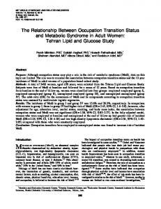
cells (Wang and Feingold, 2009a; Feingold et al., 2010). A homogeneously distributed low aerosol/droplet number concentration generates widespread precipitation and is thus the most often used method to achieve the closed- to open-cell transition. Anecdotal evidence from research scientists and pilots suggests that strong precipitation may exist in closed cellular convection. Figure 1 shows radar reflectivity measured with the ship mounted W- and C-band radars on 23 November 2008 between 07:00 and 09:00 UTC during the Variability of the American Monsoon Systems (VAMOS) Ocean Cloud Atmosphere Land Study Regional Experiment (VOCALS-REx; Wood et al., 2011b). The figure also shows the 4 km resolution infrared images observed from the Geostationary Operational Environmental Satellite (GOES). A threshold value of −15 dBZ is commonly used to indicate the existence of strong drizzle (−15 dBZ corresponds to roughly 0.1 mm d−1 rain rate; Comstock et al., 2004). In spite of persistent drizzle over the 2 h period, there is no evidence of open cellular structure – at least at the 4 km spatial resolution, and over the range of the C-band radar (∼ 100 km). Precipitation thus appears to be necessary, but not sufficient for open-cell transition (e.g., Feingold et al., 2010; Wood et al., 2011a). Feingold et al. (2010) hypothesized that the open-cell transition requires another element – sufficiently widespread precipitation. A few studies have considered aerosol gradients within horizontal domain lengths on the order of 25–100 km (Wang and Feingold, 2009b; Wang et al., 2010; Berner et al., 2013). The large characteristic length scale of organized convection requires domains much larger than those applied in typical LES. Wang and Feingold (2009b) showed that with a simulation initialized with an aerosol gradient, the outflow associated with the precipitation in open cells transported moisture toward non-precipitating closed cells. The resultant buildup of liquid water path (LWP) eventually initiated precipitation in the closed cells, with subsequent formation of open cells. Wang et al. (2010) investigated the initiation of open-cell formation with regions of lower aerosol as well as perturbations of moisture and temperature, and found that the latter initiated driz-
Abstract
Introduction
Conclusions
References
Tables
Figures
J
I
J
I
Back
Close
Full Screen / Esc Printer-friendly Version Interactive Discussion
|
25655
Discussion Paper
25
The System for Atmospheric Modeling (SAM; Khairoutdinov and Randall, 2003) is employed. SAM is formulated as an anelastic system, spatially discretized on the Arakawa C grid with a vertical height coordinate. The equations of motion are advanced with a 3rd-order Adams–Bashforth scheme (Durran, 1991), and with a 2nd-order centerdifference scheme for advection. The subgrid scale model is the 1.5-order turbulence kinetic energy scheme of Deardorff (1980). The bulk 2-moment microphysics scheme of Feingold et al. (1998) is used with a bulk sedimentation scheme following Morrison (2012), which is equivalent and more efficient that the earlier bin sedimentation scheme. Prognostic scalar variables are liquid water static energy, mixing ratios of
|
20
Model
14, 25651–25685, 2014
Relationship between open cell transition and spatial distribution of rain T. Yamaguchi and G. Feingold
Title Page
Discussion Paper
2.1
Numerical model and simulations
ACPD
|
2
Discussion Paper
15
|
10
Discussion Paper
5
zle and open-cell formation in neighboring unperturbed closed cells instead of in the perturbed area. They referred to this as a remote control of open-cell formation. In this study, we focus more closely on the idea that aerosol or precipitation gradients might play a role in the selection of the cellular state of the system. A series of idealized numerical experiments are performed to evaluate the influence of the spatial distribution of rain on the structural transition from closed to open cells. Structure is defined by particular distributions of a few key parameters. The first series of simulations is conducted to address the influence of both the formation and areal coverage of precipitation when the region of precipitation is concentrated at one location. Further numerical simulations are performed to understand the influence of multiple precipitation regions separated by some distance. A metric that quantifies the degree of open-cell transition is developed to aid in objective analysis. The next section describes the numerical model and simulations. The metric for the open-cell transition is described in Sect. 3. Results are presented in Sect. 4. Additional discussions and conclusions are given in Sects. 5 and 6, respectively.
Abstract
Introduction
Conclusions
References
Tables
Figures
J
I
J
I
Back
Close
Full Screen / Esc Printer-friendly Version Interactive Discussion
| Discussion Paper |
25656
14, 25651–25685, 2014
Relationship between open cell transition and spatial distribution of rain T. Yamaguchi and G. Feingold
Title Page
Discussion Paper
25
ACPD
|
20
Discussion Paper
15
|
10
Discussion Paper
5
water vapor, cloud water, and rain water, supersaturation, number concentrations of aerosol, cloud droplets, and rain drops, and subgrid scale turbulence kinetic energy. All scalars are transported with the monotonic 5th-order scheme of Yamaguchi et al. (2011). The model configuration is based on the Global Energy and Water Exchanges Project (GEWEX) Cloud System Study (GCSS, currently known as the Global Atmospheric System Studies (GASS)) LES intercomparison case of the Second Dynamics and Chemistry of Marine Stratocumulus (DYCOMS-II RF02; Ackerman et al., 2009) with several modifications. This is a nocturnal drizzling stratocumulus case. A horizontally square domain covers 51.2 km width with 200 m resolution and the depth of the domain is 1.6 km with 10 m vertical resolution. The lateral boundary conditions are doubly periodic. The timestep is 1 s. The initial horizontal wind is set to 0 m s−1 in order to produce horizontally stationary cell patterns (Wang and Feingold, 2009a). For consistency, the Coriolis effect is not applied. No modifications are made to the standard GCSS DYCOMS-II RF02 forcings: large-scale subsidence is computed with the specified large-scale horizontal wind divergence of 3.75 × 10⁻⁶ s−1 ; surface sensible and latent heat fluxes are constant at 16 W m−2 and 93 W m−2 , respectively; friction −1 velocity for surface momentum flux is constant and 0.25 m s ; longwave radiative flux is computed with a simple longwave radiation scheme (Ackerman et al., 2009). Simulation of mesoscale organization requires large domains, and in the current case, a large number of simulations. (The importance of large domains will become apparent.) The associated computational expense requires a CSRM approach. The relatively coarse resolution, especially in the horizontal direction, and high grid aspect ratio (horizontal to vertical grid ratio is 20 : 1) in our configuration do not fit in the realm of LES. Earlier work by Wang and Feingold (2009a) demonstrated that mesoscale circulations simulated with CSRM are qualitatively the same as their higher resolution counterparts and therefore the current choice of grid size is not expected to change the qualitative nature of results to be presented herein.
Abstract
Introduction
Conclusions
References
Tables
Figures
J
I
J
I
Back
Close
Full Screen / Esc Printer-friendly Version Interactive Discussion
Discussion Paper
5
SAM’s standard horizontal mean statistics data (time series and profiles) are recorded every minute. Posteriori 2-dimensional horizontal fields of LWP, vertically integrated droplet number concentration (Nd ), and optical depth (τ) for total liquid water (i.e., the sum of cloud and rain water) as well as rain water path (RWP) and surface rain rate are output every minute. Albedo is calculated from τ with the two stream approximation of Bohren (1987).
|
2.2
Discussion Paper |
25657
|
25
Relationship between open cell transition and spatial distribution of rain T. Yamaguchi and G. Feingold
Title Page
Discussion Paper
20
14, 25651–25685, 2014
|
15
Three series of simulations are designed for this study. The first series, S1 uses a variety of a homogeneously distributed initial aerosol number concentrations (na ), and are run for 12 h. Rain water is not allowed to precipitate over the first hour to allow turbulence to develop. S1 consists of 11 cases with different na ranging between 50 mg−1 −1 −1 −1 −3 and 250 mg in increments of 20 mg . Note that 1 mg = 1 cm at an air density −3 of 1 kg m . Each case is named with the initial na ; e.g., N070 denotes the case with na = 70 mg−1 . This series of simulations is the basis for development of the metric for closed- to open-cell transition. The second series, S2 consists of 20 cases, which all branch off from N130 of S1 at 3 h and are run for a further 9 h (i.e., for a total of 12 h). As shown in the next section, N130 is the case with the smallest initial na among S1 that maintains closed cells for 12 h. A cylinder is placed vertically in the center of the horizontal domain at 3 h. This “patch" covers a specified horizontal fractional area. Inside the patch, the total number concentration, nt , which is the sum of na and cloud water droplet number concentration (nc ), is changed to the specified value to initiate precipitation. Partitioning the specified nt to na and nc is done based on the number ratio of these two variables, i.e., na = [na /(na + nc )]nt at 3 h. The list of cases is presented in Table 1. Each case is named according to the horizontal fractional area and nt , e.g., F015-N030 denotes a patch fractional area of 0.15 and nt = 30 mg−1 .
Discussion Paper
10
Numerical simulations
ACPD
Abstract
Introduction
Conclusions
References
Tables
Figures
J
I
J
I
Back
Close
Full Screen / Esc Printer-friendly Version Interactive Discussion
| Discussion Paper |
25658
14, 25651–25685, 2014
Relationship between open cell transition and spatial distribution of rain T. Yamaguchi and G. Feingold
Title Page
Discussion Paper
25
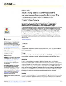
Albedo fields for N090, N110, and N130 for series S1 at 4, 8, and 12 h are presented in Fig. 2. It is clear that N090 transfers into an open cell field, while N130 remains in the closed-cell state. Domain mean statistics for all S1 cases are presented in Fig. 3. The closed-cell cases (na ≥ 130 mg−1 ) maintain LWP & 100 g m−2 and negligibly small RWP. For the last hour, well mixed profiles are present for these cases. Although very subtle, the larger initial na result in deeper boundary layers, higher cloud bases, and smaller liquid water content. This is related to entrainment resulting in faster evaporation for the higher nc (and na ) (Wang et al., 2003; Xue and Feingold, 2006; Bretherton et al., 2007; Xue et al., 2008; Hill et al., 2009). The open-cell cases (na ≤ 90 mg−1 ) show the runaway precipitation feedback discussed by Feingold and Kreidenweis (2002); LWP decreases rapidly while RWP in−2 creases rapidly to values on the order of 10 g m , and precipitation rates exceeds −1 0.5 mm day at the surface. For the last 2 h, the fields reach a steady state. The well-mixed profiles disappear for these cases and they have substantially lower PBL height due to precipitation suppressing entrainment (Stevens et al., 1998). Profiles are
ACPD
|
20
Metric for structural transition from closed to open cells
Discussion Paper
15
3
|
10
Discussion Paper
5
The third series, S3 also branches off from N130 of S1 at 3 h, but uses a horizontal domain twice as large (102.4 km width). It is also run for a further 9 h. The simulations consists of 4 cases: one case uses a single patch, and the other 3 cases place 1 patch at the domain center and 6 patches at the vertices of the hexagon whose center is located at the domain center. The inter-patch distance, i.e., the shortest distance between two patches differs among these 3 cases. The total horizontal area fraction of patches is constant among the cases and is set to 0.04. The total number concentration −1 of patches is also constant amongst the cases and is set to 30 mg . The list of cases is shown in Table 2.
Abstract
Introduction
Conclusions
References
Tables
Figures
J
I
J
I
Back
Close
Full Screen / Esc Printer-friendly Version Interactive Discussion
25659
|
14, 25651–25685, 2014
Relationship between open cell transition and spatial distribution of rain T. Yamaguchi and G. Feingold
Title Page
Discussion Paper | Discussion Paper
25
ACPD
|
20
Discussion Paper
15
|
10
Discussion Paper
5
in agreement with past studies (Savic-Jovcic and Stevens, 2008; Wang and Feingold, 2009a). N110 is interesting in that it does not quite fit into either category. At 12 h, LWP is similar to the closed-cell cases, but in contrast RWP is close to the open-cell cases, and there is negligible domain mean surface precipitation. Profiles for the thermodynamic variables are very similar to the closed-cell cases but slightly less well-mixed. Turbulence profiles differ from the closed-cell cases, which suggests that N110 completes the 12 h simulation in the middle of the transition. Looking back at the albedo fields of N110 at 12 h (Fig. 2), bright cellular lines of clouds exist, as observed in N090 at 4 h (notwithstanding the different cell sizes). These bright lines do not exist in N130 for the duration of the simulation. Wood and Hartmann (2006) developed a neural network scene classification method based on the distribution and power spectrum of LWP. This elaborate method classified a satellite image into one of four categories: no clear identifiable cellularity, closed cells, open cells, and clouds containing cells without organization. We have developed an alternative scheme that yields information on the degree of transition between closed- and open-cell structures. In order to develop a metric for open-cell transition, the time evolution of the distributions of LWP, Nd , and τ are considered. To build a simple method, and possibly apply the metric to observational data in the future, we focus on cloud fields that can be measured or derived remotely, and avoid turbulence statistics. Figure 4a shows the LWP distribution for N090 between 2.5 and 4.5 h. It is roughly approximated by a unimodal distribution at 2.5 h; with time, the distribution develops bimodality but by 4.5 h it transitions back to a unimodal distribution with a mode at the smallest bin. These two unimodal structures were also shown in observations (Wood and Hartmann, 2006; Wood et al., 2011a). For a binned distribution, the mode M is defined as the value of the bin with the highest frequency (or count). Thus, the mode for LWP is quantified with M = xi , where xi is the value of the i th LWP bin. The time series of the mode based on LWP is shown in Fig. 4b for selected cases. For the open-cell cases (N070 and N090), there is a change from the mode associated with the closed-
Abstract
Introduction
Conclusions
References
Tables
Figures
J
I
J
I
Back
Close
Full Screen / Esc Printer-friendly Version Interactive Discussion
5
14, 25651–25685, 2014
Relationship between open cell transition and spatial distribution of rain T. Yamaguchi and G. Feingold
Title Page
| Discussion Paper
25
|
where f is the frequency and f0 = fn = 0 (boundary condition). By definition, I = 1 for a pure unimodal distribution, and I = 2 for a pure bimodal distribution. Both mode and mode index are sensitive to bin size. Consider a histogram with a bin size containing either 0 or 1 counts in each bin. For this case, the number of modes, NM , equals the number of elements, and I ≥ 2. (A special case is I = 1 when f = 1 for all bins except x0 and xn .) At the other extreme, for a large enough bin size containing all elements in a single bin NM = 1 and I = 1. Considering these bounding cases, bin size is determined as follows: to find the smallest bin size, the condition is imposed that I < 1.1 at any time after spinup for N130 (a closed-cell case). This bin size is, then, applied to all S1 cases and for each case max(NM ) is identified from the time series of NM after spinup. The bin size is incrementally increased until max(NM ) ≤ 2 is satisfied for all cases. The bin sizes for LWP, Nd , and τ are 4 g m−2 , 800 mm−2 , and 0.5, respectively. These are useful, ad hoc criteria and may need to be modified for different cases. The time series of the mode indices for LWP, Nd , and τ are presented in Fig. 4c for selected cases. After rain starts to reach the surface at 1 h, the mode indices for the open-cell cases (N070 and N090) pass a peak, which exceeds 1.1 for all variables. After 10 h, the mode indices for N110 increase to a value larger than 1.1. Since at 12 h 25660
Discussion Paper
20
i =1
ACPD
|
15
(1)
Discussion Paper
10
X 1 |fi − fi −1 | 2 max(f )
|
n
I≡
Discussion Paper
−2
cellular state (M & 100 g m ) to the mode associated with the open-cellular state (the −2 first bin, x1 , i.e., M = 4 g m ). The change of mode never takes place for the closedcell case (N130). The mode change is in progress for N110 when the run ends. Thus, the differences between these two unimodal distributions reflect structural differences between closed and open-cellular states. Tracking the mode gives an indication of the timing of the transition to open cells. It can not, however, distinguish between closed cells, open cells, or the point of transition. Therefore we introduce the mode index, defined as
Abstract
Introduction
Conclusions
References
Tables
Figures
J
I
J
I
Back
Close
Full Screen / Esc Printer-friendly Version Interactive Discussion
14, 25651–25685, 2014
Relationship between open cell transition and spatial distribution of rain T. Yamaguchi and G. Feingold
Title Page
open cells when M = x1 and I < 1.1.
(2)
Discussion Paper |
25661
|
The structural classification is performed for LWP, Nd , and τ. For instance, for N110 at 12 h, the metric gives “closed cells under transition” for each variable (Fig. 4c). Although for 4 classified states and 3 variables, mathematically the total number of possible combination of states is 64, in reality there are far fewer possibilities since many combinations of states do not exist, e.g., closed cell classification based on LWP and open cell classification based on the other two variables.
Discussion Paper
closed cells under transition when M 6= x1 and I ≥ 1.1, open cells under transition when M = x1 and I ≥ 1.1, and
20
ACPD
|
15
Discussion Paper
closed cells when M 6= x1 and I < 1.1,
|
10
Discussion Paper
5
the modes of N110 do not reach x1 (Fig. 4b for LWP), the structure during transition is expected to be somewhat similar to the closed cells, as confirmed by Fig. 2. For the open-cell cases, there is a time lag for the appearance of the peak depending on the variable under consideration, i.e., LWP, Nd or τ: LWP comes first, followed by τ, and finally Nd . Thus the amount of condensate is a stronger indicator of the beginning of a transition than is a microphysical property such as Nd . τ is a blend of condensate and microphysical properties and therefore appears second. This ordering may be partially related to the selected bin sizes and we do not place much emphasis on this result. The selection of the three different parameters is primarily to assess robustness of the transition metric. With the mode and mode index, four states can be classified for each variable: closed cells, closed cells under transition, open cells under transition, and open cells. The four states are classified as follows:
Abstract
Introduction
Conclusions
References
Tables
Figures
J
I
J
I
Back
Close
Full Screen / Esc Printer-friendly Version Interactive Discussion
4.1
5
14, 25651–25685, 2014
Relationship between open cell transition and spatial distribution of rain T. Yamaguchi and G. Feingold
Title Page
Discussion Paper | Discussion Paper
25
ACPD
|
20
|
The time evolution of albedo for selected S2 cases is shown in Fig. 5. Based on the metrics, all 20 cases are categorized into only 5 combinations of classified states from closed to open cells. Unlike the open-cell cases for S1, there is no clear cellular pattern for the open-cell case (F015-N030) at 12 h, however the metric suggests that the structure strongly resembles that of open cells based on the distribution of LWP, Nd and τ. For the closed-cell case (F010-N090), the patch is completely swallowed by surrounding cloudy air. For the open-cell (left) and transition cases (3 central columns), the divergence (or outflow from the domain center) created by the precipitation propagates outward and a low albedo area develops. That outflow propagates back toward the domain center once it reaches the horizontal boundary due to periodicity; this effect is examined later in Sect. 5. Figure 6a shows the evolution of RWP between 6 and 10 h for F015-N030. The propagation of the RWP is approximately symmetrical since the patch is introduced at the domain center. As seen at 9 h, the distortion of the symmetry happens once the propagation reaches the domain boundary. Due to this quasi-symmetry, we calculate the radially averaged RWP, with the radius measured from the domain center, and plot this field as a modified Hovmöller diagram. Figure 6b shows the Hovmöller diagram of radially averaged RWP for three S2 cases. It captures the dynamical response of the generation of new raining areas due to convergence of outflows produced by precipitation. For F015-N030 and F010-N050, the onset of precipitation first creates a RWP convergence region at approximately 4 km radius (slightly less than the radius of the patch) and 4.5 h, then the second RWP concentrated region forms near the domain center (i.e., 0 km radius) at 5.5 h. The second region persists longer than the first convergence region. The third region appears at approximately 16 km radius and 7.5 h after the second region has disappeared. After the third convergence, the perturbation reaches the horizontal boundary and proceeds inward to the domain center. Note that 25662
Discussion Paper
15
Single patch simulations
|
10
Results
Discussion Paper
4
Abstract
Introduction
Conclusions
References
Tables
Figures
J
I
J
I
Back
Close
Full Screen / Esc Printer-friendly Version Interactive Discussion
Discussion Paper |
To explore the effect of multiple rain regions on the open-cell transition, the S3 simulations (Sect. 2, Table 2) are now discussed. The difference in the model configurations compared to the other simulations is that the horizontal domain size is extended to 102.4 × 102.4 km2 . This large domain is required to fit distributed patches in the domain, as well as to avoid a bias caused by the periodic boundary conditions. As noted earlier, the outflow sometimes reaches the domain edge before the simulation ends 25663
|
25
Multiple patch simulations
14, 25651–25685, 2014
Relationship between open cell transition and spatial distribution of rain T. Yamaguchi and G. Feingold
Title Page
Discussion Paper
4.2
ACPD
|
20
Discussion Paper
15
|
10
Discussion Paper
5
the closed-cell case (F010-N090) evolves in a similar way, albeit with slow propagation speed and weak magnitude, and it also manages to create the third precipitating region towards the end of the simulation. Results of the metrics for the open-cell transition applied to the all S2 cases at 12 h are presented in Fig. 7. For a given fractional area, a larger gradient in nt between the environment and the patch leads to the formation of open cells, and for a given gradient, a larger fractional area leads to the formation of open cells. Although the number of cases is limited, the results suggest that the gradient of nt and the areal coverage of rain are of similar importance for the open-cell transition. To capture the features discussed for S1 (Fig. 4b and c), time series of the mode and mode index are shown in Fig. 8a for selected S2 cases. It is noted that (i) the case with an earlier LWP mode change also arrives earlier back to a mode index of 1.1, (ii) because of the limited patch sizes, complete transition requires a long period of time – the fastest transition amongst the S2 cases (i.e., F020-N010, not shown in the figure) takes approximately 7 h based on these metrics. Transition times were much shorter in the S1 simulations (Fig. 4). Figure 8b shows the time series of surface precipitation rate for domain mean and conditional mean. For the domain mean, the closed-cell case seems not to precipitate; −1 −1 its conditional average (over rain rates > 0.1 mm day ), however, exceeds 2 mm day , which suggests that the locally measured surface rain rate should not be considered a priori an indicator of open cells.
Abstract
Introduction
Conclusions
References
Tables
Figures
J
I
J
I
Back
Close
Full Screen / Esc Printer-friendly Version Interactive Discussion
25664
|
14, 25651–25685, 2014
Relationship between open cell transition and spatial distribution of rain T. Yamaguchi and G. Feingold
Title Page
Discussion Paper | Discussion Paper
25
ACPD
|
20
Discussion Paper
15
|
10
Discussion Paper
5
and propagates inward to the domain, which essentially “contaminates” the flow. Note that nt of patches is 30 mg−1 for all cases. Figure 9 shows the evolution of the albedo for all S3 cases. The metrics applied for 2 2 a 51.2 × 51.2 km subdomain and the full domain (102.4 × 102.4 km ) at 12 h are also shown in schematic form. SP reaches an open-cell state based on the metric applied to the subdomain, which is anticipated since the areal fraction of 0.04 for the full domain is equivalent to that of 0.16 for the domain with 51.2 km width. Simulation F015-N030 2 of S2 (single patch covering 0.15 area fraction for the 51.2 × 51.2 km domain) also achieves an open-cell state (Fig. 7). The transition occurs via interactions between precipitation-generated outflows associated with the patches in H1, H2, and H3; these patches are not able to transform to open cells without these interactions. This is anticipated since each patch only covers an areal fraction of approximately 0.006, which translates to 0.023 for the domain with 51.2 km width, and as shown above, F005-N030 2 of S2 (single patch covering 0.05 area fraction for the 51.2 × 51.2 km domain) remains in the closed-cell state (Fig. 7). The transition for H3 is the slowest amongst the cases due to the largest distance between patches. This is because the outflows have to travel the longest distance to converge with other outflows. The open areas of H3 are completely filled by surrounding cloudy air, but by 12 h open areas have appeared. For much larger inter-patch distances (all else equal) the outflows are not able to create strong enough updrafts at the convergence zones, the transition comes to a halt, and the system returns to the closed-cell state. How widely the rainy areas spread for a given duration is determined by the distance between the outer edge of the precipitating area (the “rim”) and the domain boundary (hereafter, rim-boundary distance) as well as the inter-patch distance. The effect appears in the differences among the metrics in Fig. 9. For the rim-boundary distance, SP > H1 > H2 > H3, and for the inter-patch distance, H1 < H2 < H3. SP initiates precipitation within the patch, which produces relatively strong dynamical feedback within the subdomain, but the case requires time to propagate rain regions to the outer reaches of the domain because of the large rim-boundary distance. On the other hand, the
Abstract
Introduction
Conclusions
References
Tables
Figures
J
I
J
I
Back
Close
Full Screen / Esc Printer-friendly Version Interactive Discussion
| Discussion Paper |
25665
14, 25651–25685, 2014
Relationship between open cell transition and spatial distribution of rain T. Yamaguchi and G. Feingold
Title Page
Discussion Paper
25
ACPD
|
20
Discussion Paper
15
|
10
Discussion Paper
5
rim-boundary and inter-patch distances for H1 are optimal for spreading rain regions outward through dynamical response. Relative to SP, it does, however, require more time to fully transform the H1 subdomain into an open-cell state. The dynamical feedback is shown in Fig. 10a in the form of a Hovmöller diagram of RWP. The wavelike pattern for SP is different from that for H1. SP creates a relatively short lived convergence at the domain center at approximately 6.5 h, and later a strong domain center convergence at approximately 11.5 h after the inflow from the rain area located at approximately 15 km radius arrives at the domain center. H1 shows convergence at approximately half of the distance between patches (6.5 km radius) at 5 h following the initial rain event; then the large RWP associated with strong convergence at the domain center forms at approximately 6 h and spreads outward. H2 and H3 exhibit a similar evolution, but with slower phase speed since the inter-patch distance is longer. Figure 10b shows that strong, coherent surface rain occurs when the RWP −1 convergence exists, and that H1 produces surface precipitation of > 4.5 mm d while −1 SP and all but two cases of S2 (Fig. 8b) do not produce surface rain > 3.5 mm d . H2 −1 and H3 produce surface precipitation > 4.5 mm d (not shown). These strong precipitation events for the multipatch cases occur at the large RWP convergence zones at the domain center, e.g., at 7 h for H1. SP has the largest convergence at 11.5 h and the surface rain rate is at its maximum. The rain rate difference between these convergence zones can be shown to be related to the distance to the domain center from the previous convergence, which is the source of outflow traveling toward the domain center. Although the surface rain rates for the previous convergence for H1 and SP are −1 similar to each other and approximately 2 mm d , the previous convergence for H1 is located much closer to the domain center than that for SP, allowing the outflow to generate stronger updrafts.
Abstract
Introduction
Conclusions
References
Tables
Figures
J
I
J
I
Back
Close
Full Screen / Esc Printer-friendly Version Interactive Discussion
5
| Discussion Paper |
25666
14, 25651–25685, 2014
Relationship between open cell transition and spatial distribution of rain T. Yamaguchi and G. Feingold
Title Page
Discussion Paper
25
ACPD
|
20
Discussion Paper
15
Berner et al. (2013) used multi-day, 2-dimensional CSRM simulations to study the slow manifold path toward a shallow broken, or deeper well-mixed stratocumulus capped PBL with adjustment time scales of several days. In the spirit of synthesizing model output of system evolution, we consider a phase diagram for the mean and coefficient of variation, cv , (i.e., standard deviation divided by the mean) for LWP, Nd , and τ. Relationships between the mean and variance of cloud fields are especially useful for boundary-layer parameterizations employed in climate models. We show here that in this phase-space the different model configurations exhibit a predictable evolutionary pathway when perturbed by low aerosol concentration patches. Figure 11 shows the phase diagram for the mean and cv , for LWP, Nd , and τ for all cases of S1 (Fig. 11a), S2 (Fig. 11b), and S3 (Fig. 11c) for the entire duration of the simulations (12 h for S1, 9 h for S2 and S3). The calculation of cv and mean for S3 is performed on the 51.2 × 51.2 km2 subdomain. −1 For S1 (Fig. 11a), cv for the closed-cell cases (na > 130 mg , red colored) remains small while the mean decreases in response to a deepening of the boundary layer, and entrainment reducing the cloud water (Fig. 3). For the open-cell cases (na < 90 mg−1 , blue colored), the pathways converge to one curve, characterized by a decreasing −1 mean and an increasing cv . The transition case (na = 110 mg , green colored) also merges to the open-cell phase curve. It is noted that the rate of cv increase for opencell cases is larger for smaller initial na (not shown). It is also worth noting that the phase diagrams for the skewness vs. the mean also form a single curve (not shown). The phase curves for S2 (Fig. 11b) exhibit similar behavior. They form a characteristic curve, which is independent of the area fraction or patch-environment gradient in nt . More interestingly, the phase curve for LWP for S2 overlaps that of S1. The behavior for Nd and τ is somewhat different. Recall that, for S2, when a patch is introduced, the liquid water mass mixing ratio is not altered but the number concentration is. This leads to initially higher cv for Nd or τ as a result of both larger standard deviation and smaller
|
10
Predictable transition pathway?
Discussion Paper
5
Abstract
Introduction
Conclusions
References
Tables
Figures
J
I
J
I
Back
Close
Full Screen / Esc Printer-friendly Version Interactive Discussion
Discussion Paper |
25667
|
25
14, 25651–25685, 2014
Relationship between open cell transition and spatial distribution of rain T. Yamaguchi and G. Feingold
Title Page
Discussion Paper
20
The main goal of this work is to test the hypothesis posed by Feingold et al. (2010) that precipitation is not a sufficient condition for the formation of open cells in conditions conducive to closed-cellular convection, but that the spatial distribution of precipitation plays a role. To explore the effect of the spatial distribution of precipitation on the formation of open cells, a series of idealized simulations are performed by inserting single or multiple patches with reduced nt into the closed-cell field. A simple metric for closedto open-cell transition is developed; the metric could be applied to satellite-based observations of cloud fields, especially geostationary satellites. For the simulations with single patches (S2), relatively strong, localized precipitation events (order 2 mm day−1 ) are insufficient to initiate transition to open cells. In general, the transformation to open cells occurs for sufficiently small nt and/or large patch area fraction. Both of these factors appear to be of similar importance. For the simulations with multiple patches (S3), the inter-patch distance selects the resulting state for patches that alone are too weak to initiate the open-cell transformation. When patches are close to one another, interactions between precipitation-driven outflows bolster the transition to open cells, whereas when they are separated by large enough distances,
ACPD
|
15
Conclusions
Discussion Paper
6
|
10
Discussion Paper
5
mean compared with S1, and a trajectory that lies above that of S1. At higher cv the S2 phase curves for Nd and τ merge to those of S1. The effect of domain size can be seen in Fig. 11c. All S3 cases again form one phase curve, which starts at approximately the same mean and cv as in S2, but deviates later. Since F015-N030 of S2 and SP of S3 only differ by 0.01 area fraction for the 51.2 km domain width, without the bias arising from the domain size the shadings for S2 and S3 should overlap each other for the entire duration of the simulation. One can see here that the bias associated with periodic boundary conditions and the associated premature inward propagation of the outflow generated by precipitation hastens the transition from closed to open cell.
Abstract
Introduction
Conclusions
References
Tables
Figures
J
I
J
I
Back
Close
Full Screen / Esc Printer-friendly Version Interactive Discussion
Discussion Paper |
25668
|
Acknowledgements. This study is supported by the NOAA Climate Program Office. Thanks are due to C. Fairall for the W-band data and S. Yuter for the C-band data. The authors thank Jan Kazil for insightful discussions. T. Yamaguchi was supported by a NOAA and NSF funded Climate Process Team grant (V. Larson, PI).
14, 25651–25685, 2014
Relationship between open cell transition and spatial distribution of rain T. Yamaguchi and G. Feingold
Title Page
Discussion Paper
25
ACPD
|
20
Discussion Paper
15
|
10
Discussion Paper
5
the transition is less effective. Large enough distances of separation can be viewed as localized raining areas which, based on the S2 simulations, unless strong and large enough, will not transition the system to open cells. Modified Hovmöller diagrams of the radially averaged RWP show wavelike patterns, with rainy regions migrating back and forth between the domain center and the outer reaches of the domain. This wavelike behavior is associated with what Wang et al. (2010) called a remote control of open-cell formation; perturbations or existing open cells generate moisture convergence into the surrounding unperturbed closed-cell region, initiate precipitation there, and result in open-cell formation. Furthermore, multiple patches can accomplish this remote control when one patch is not able to achieve this. We further anticipate that (i) if the perturbation is strong enough, the remote control probably propagates more effectively, forming open cells without additional support, and (ii) if multiple remote controls occur simultaneously, interaction of these remote controls could enhance the formation of open cells over a wider area. Following the idea of slow manifolds of Bretherton et al. (2010), we show that the phase diagrams of the coefficient of variation and mean cloud field properties of LWP, Nd , and τ follow one phase trajectory for given large scale meteorological conditions. The extent to which the phase trajectory is consistent for a range of different meteorological states is left for future research. In summary, we have shown here that strong, localized surface rain (order 2 mm day−1 ) is not a sufficient condition for a transition from the closed- to the open-cell state. Both the gradient of nt and the areal coverage of rain are of equal importance for initiating this transition. Interacting patches, if close enough to one another, also facilitate the transition. Further research will use satellite-based data to test this hypothesis, as well as the existence of preferred variance vs. mean phase trajectories.
Abstract
Introduction
Conclusions
References
Tables
Figures
J
I
J
I
Back
Close
Full Screen / Esc Printer-friendly Version Interactive Discussion
5
Discussion Paper |
25669
|
30
14, 25651–25685, 2014
Relationship between open cell transition and spatial distribution of rain T. Yamaguchi and G. Feingold
Title Page
Discussion Paper
25
ACPD
|
20
Discussion Paper
15
|
10
Ackerman, A. S., vanZanten, M. C., Stevens, B., Savic-Jovcic, V., Bretherton, C. S., Chlond, A., Golaz, J.-C., Jiang, H., Khairoutdinov, M., Krueger, S. K., Lewellen, D. C., Lock, A., Moeng, C.-H., Nakamura, K., Petters, M. D., Snider, J. R., Weinbrecht, S., and Zulauf, M.: Large-eddy simulations of a drizzling, stratocumulus-topped marine boundary layer, Mon. Weather Rev., 137, 1083–1110, 2009. 25656 Berner, A. H., Bretherton, C. S., and Wood, R.: Large-eddy simulation of mesoscale dynamics and entrainment around a pocket of open cells observed in VOCALS-REx RF06, Atmos. Chem. Phys., 11, 10525–10540, doi:10.5194/acp-11-10525-2011, 2011. 25653 Berner, A. H., Bretherton, C. S., Wood, R., and Muhlbauer, A.: Marine boundary layer cloud regimes and POC formation in a CRM coupled to a bulk aerosol scheme, Atmos. Chem. Phys., 13, 12549–12572, doi:10.5194/acp-13-12549-2013, 2013. 25653, 25654, 25666 Bohren, C. F.: Multiple scattering of light and some of its observable consequences, Am. J. Phys., 55, 524–533, 1987. 25657 Bretherton, C. S., Blossey, P. N., and Uchida, J.: Cloud droplet sedimentation, entrainment efficiency, and subtropical stratocumulus albedo, Geophys. Res. Lett., 34, L03813, doi:10.1029/2006GL027648, 2007. 25658 Bretherton, C. S., Uchida, J., and Blossey, P. N.: Slow manifolds and multiple equilibria in stratocumulus-capped boundary layers, J. Adv. Model. Earth Syst., 2, 14 pp., doi:10.3894/JAMES.2010.2.14, 2010. 25668 Comstock, K. K., Wood, R., Yuter, S. E., and Bretherton, C. S.: Reflectivity and rain rate in and below drizzling stratocumulus, Q. J. Roy. Meteor. Soc., 130, 2891–2918, 2004. 25654 Comstock, K. K., Bretherton, C. S., and Yuter, S. E.: Mesoscale variability and drizzle in southeast Pacific stratocumulus, J. Atmos. Sci., 62, 3792–3807, 2005. 25653 Deardorff, J. W.: Stratocumulus-capped mixed layers derived from a three-dimensional model, Bound.-Lay. Meteor., 18, 495–527, 1980. 25655 Durran, D. R.: The third-order Adams–Bashforth method: an attractive alternative to leapfrog time differencing, Mon. Weather Rev., 119, 702–720, 1991. 25655 Feingold, G. and Koren, I.: A model of coupled oscillators applied to the aerosol-cloudprecipitation system, Nonlinear Proc. Geoph., 20, 1011–1021, 2013. 25653
Discussion Paper
References
Abstract
Introduction
Conclusions
References
Tables
Figures
J
I
J
I
Back
Close
Full Screen / Esc Printer-friendly Version Interactive Discussion
Discussion Paper |
25670
|
30
14, 25651–25685, 2014
Relationship between open cell transition and spatial distribution of rain T. Yamaguchi and G. Feingold
Title Page
Discussion Paper
25
ACPD
|
20
Discussion Paper
15
|
10
Discussion Paper
5
Feingold, G. and Kreidenweis, S. M.: Cloud processing of aerosol as modeled by a large eddy simulation with coupled microphysics and aqueous chemistry, J. Geophys. Res., 107, 4687, doi:10.1029/2002JD002054, 2002. 25658 Feingold, G., Walko, R. L., Stevens, B., and Cotton, W. R.: Simulations of marine stratocumulus using a new microphysical parameterization scheme, Atmos. Res., 47–48, 505–528, 1998. 25655 Feingold, G., Koren, I., Wang, H., Xue, H., and Brewer, W. A.: Precipitation-generated oscillations in open cellular cloud fields, Nature, 466, 849–852, 2010. 25653, 25654, 25667 Hill, A. A., Feingold, G., and Jiang, H.: The influence of entrainment and mixing assumption on aerosol-cloud interactions in marine stratocumulus, J. Atmos. Sci., 66, 1450–1464, 2009. 25658 Kazil, J., Wang, H., Feingold, G., Clarke, A. D., Snider, J. R., and Bandy, A. R.: Modeling chemical and aerosol processes in the transition from closed to open cells during VOCALSREx, Atmos. Chem. Phys., 11, 7491–7514, doi:10.5194/acp-11-7491-2011, 2011. 25653 Khairoutdinov, M. F. and Randall, D. A.: Cloud resolving modeling of the ARM summer 1997 IOP: model formulation, results, uncertainties, and sensitivities, J. Atmos. Sci., 60, 607–625, 2003. 25655 Koren, I. and Feingold, G.: Aerosol-cloud-precipitation system as a predator-prey problem, P. Natl. Acad. Sci. USA, 108, 12227–12232, doi:10.1073/pnas.1101777108, 2011. 25653 Mechem, D. B., Yuter, S. E., and De Szoeke, S. P.: Thermodynamic and aerosol controls in southeast Pacific stratocumulus, J. Atmos. Sci., 69, 1250–1266, 2012. 25653 Morrison, H.: On the numerical treatment of hydrometeor sedimentation in bulk and hybrid bulk-bin microphysics schemes, Mon. Weather Rev., 140, 1572–1588, 2012. 25655 Ovchinnikov, M., Easter, R. C., and Gustafson, W. I.: Untangling dynamical and microphysical controls for the structure of stratocumulus, Geophys. Res. Lett., 40, 4432–4436, 2013. 25653 Petters, M. D., Snider, J. R., Stevens, B., Vali, G., Faloona, I., and Russell, L. M.: Accumulation mode aerosol, pockets of open cells, and particle nucleation in the remote subtropical Pacific marine boundary layer, J. Geophys. Res., 111, D02206, doi:10.1029/2004JD005694, 2006. 25653 Savic-Jovcic, V. and Stevens, B.: The structure and mesoscale organization of precipitating stratocumulus, J. Atmos. Sci., 65, 1587–1605, 2008. 25653, 25659
Abstract
Introduction
Conclusions
References
Tables
Figures
J
I
J
I
Back
Close
Full Screen / Esc Printer-friendly Version Interactive Discussion
Discussion Paper |
25671
|
30
14, 25651–25685, 2014
Relationship between open cell transition and spatial distribution of rain T. Yamaguchi and G. Feingold
Title Page
Discussion Paper
25
ACPD
|
20
Discussion Paper
15
|
10
Discussion Paper
5
Sharon, T. M., Albrecht, B. A., Jonsson, H. H., Minnis, P., Khaiyer, M. M., van Reken, T. M., Seinfeld, J., and Flagan, R.: Aerosol and cloud microphysical characteristics of rifts and gradients in maritime stratocumulus clouds, J. Atmos. Sci., 63, 983–997, 2006. 25653 Stevens, B., Cotton, W. R., Feingold, G., and Moeng, C.-H.: Large-Eddy simulations of strongly precipitating, shallow, stratocumulus-topped boundary layers, J. Atmos. Sci., 55, 3616–3638, 1998. 25658 Stevens, B., Vali, G., Comstock, K., Wood, R., Van Zanten, M. C., Austin, P. H., Bretherton, C. S., and Lenschow, D. H.: Pockets of open cells and drizzle in marine stratocumulus, B. Am. Meteorol. Soc., 86, 51–57, 2005. 25653 Terai, C. R., Bretherton, C. S., Wood, R., and Painter, G.: Aircraft observations of aerosol, cloud, precipitation, and boundary layer properties in pockets of open cells over the southeast Pacific, Atmos. Chem. Phys., 14, 8071–8088, doi:10.5194/acp-14-8071-2014, 2014. 25653 vanZanten, M. C. and Stevens, B.: Observations of the structure of heavily precipitating marine stratocumulus, J. Atmos. Sci., 62, 4327–4342, 2005. 25653 Wang, H. and Feingold, G.: Modeling mesoscale cellular structures and drizzle in marine stratocumulus. Part I: Impact of drizzle on the formation and evolution of open cells, J. Atmos. Sci., 66, 3237–3256, 2009a. 25653, 25654, 25656, 25659 Wang, H. and Feingold, G.: Modeling mesoscale cellular structures and drizzle in marine stratocumulus. Part II: The microphysics and dynamics of the boundary region between open and closed cells, J. Atmos. Sci., 66, 3257–3275, 2009b. 25653, 25654 Wang, H., Feingold, G., Wood, R., and Kazil, J.: Modelling microphysical and meteorological controls on precipitation and cloud cellular structures in Southeast Pacific stratocumulus, Atmos. Chem. Phys., 10, 6347–6362, doi:10.5194/acp-10-6347-2010, 2010. 25653, 25654, 25668 Wang, S., Wang, Q., and Feingold, G.: Turbulence, condensation, and liquid water transport in numerically simulated nonprecipitating stratocumulus clouds, J. Atmos. Sci., 60, 262–278, 2003. 25658 Wood, R. and Hartmann, D. L.: Spatial variability of liquid water path in marine low cloud: the importance of mesoscale cellular convection, J. Climate, 19, 1748–1764, 2006. 25659 Wood, R., Comstock, K. K., Bretherton, C. S., Cornish, C., Tomlinson, J., Collins, D. R., and Fairall, C.: Open cellular structure in marine stratocumulus sheets, J. Geophys. Res., 113, D12207, doi:10.1029/2007JD009371, 2008. 25653
Abstract
Introduction
Conclusions
References
Tables
Figures
J
I
J
I
Back
Close
Full Screen / Esc Printer-friendly Version Interactive Discussion
Discussion Paper
15
|
10
Discussion Paper
5
14, 25651–25685, 2014
Relationship between open cell transition and spatial distribution of rain T. Yamaguchi and G. Feingold
Title Page
Discussion Paper | Discussion Paper |
25672
ACPD
|
Wood, R., Bretherton, C. S., Leon, D., Clarke, A. D., Zuidema, P., Allen, G., and Coe, H.: An aircraft case study of the spatial transition from closed to open mesoscale cellular convection over the Southeast Pacific, Atmos. Chem. Phys., 11, 2341–2370, doi:10.5194/acp-11-23412011, 2011a. 25653, 25654, 25659 Wood, R., Mechoso, C. R., Bretherton, C. S., Weller, R. A., Huebert, B., Straneo, F., Albrecht, B. A., Coe, H., Allen, G., Vaughan, G., Daum, P., Fairall, C., Chand, D., Gallardo Klenner, L., Garreaud, R., Grados, C., Covert, D. S., Bates, T. S., Krejci, R., Russell, L. M., de Szoeke, S., Brewer, A., Yuter, S. E., Springston, S. R., Chaigneau, A., Toniazzo, T., Minnis, P., Palikonda, R., Abel, S. J., Brown, W. O. J., Williams, S., Fochesatto, J., Brioude, J., and Bower, K. N.: The VAMOS Ocean-Cloud-Atmosphere-Land Study Regional Experiment (VOCALS-REx): goals, platforms, and field operations, Atmos. Chem. Phys., 11, 627–654, doi:10.5194/acp-11-627-2011, 2011b. 25654 Xue, H. and Feingold, G.: Large-eddy simulations of trade wind cumuli: investigation of aerosol indirect effects, J. Atmos. Sci., 63, 1605–1622, 2006. 25658 Xue, H., Feingold, G., and Stevens, B.: Aerosol effects on clouds, precipitation, and the organization of shallow cumulus convection, J. Atmos. Sci., 65, 392–406, 2008. 25653, 25658 Yamaguchi, T., Randall, D. A., and Khairoutdinov, M. F.: Cloud modeling tests of the ULTIMATEMACHO scalar advection scheme, Mon. Weather Rev., 139, 3248–3264, 2011. 25656
Abstract
Introduction
Conclusions
References
Tables
Figures
J
I
J
I
Back
Close
Full Screen / Esc Printer-friendly Version Interactive Discussion
Discussion Paper | Discussion Paper
Table 1. List of cases for S2 simulations with a variety of single patches placed at the domain center. Each case branches off from N130 of S1 at 3 h, and is run for 9 h. Case name represents specified fractional area and nt of the patch. F015-N030 uses a patch with area fraction of 0.15 −1 and nt = 30 mg .
ACPD 14, 25651–25685, 2014
Relationship between open cell transition and spatial distribution of rain T. Yamaguchi and G. Feingold
Title Page
radius (km)
nt (mg )
0.05 0.10 0.15 0.20
6.46 9.13 11.19 12.92
10, 30, 50, 70, 90 10, 30, 50, 70, 90 10, 30, 50, 70, 90 10, 30, 50, 70, 90
Discussion Paper
F005-N0.. F010-N0.. F015-N0.. F020-N0..
fractional area
|
Case
−1
| Discussion Paper |
25673
Abstract
Introduction
Conclusions
References
Tables
Figures
J
I
J
I
Back
Close
Full Screen / Esc Printer-friendly Version Interactive Discussion
Discussion Paper | Discussion Paper
Table 2. List of cases for S3 simulations for multiple patches. Each case branches off from N130 of S1 at 3 h, performed with the large domain (102.4 km domain width), and is run for −1 9 h. The total area fraction covered by the patches is 0.04 and nt = 30 mg . The inter-patch distance is the shortest distance between the sides of two patches.
ACPD 14, 25651–25685, 2014
Relationship between open cell transition and spatial distribution of rain T. Yamaguchi and G. Feingold
Title Page
|
Case
radius (km)
inter-patch distance (km)
single patch hexagon (6 at vertices, 1 at center) hexagon (6 at vertices, 1 at center) hexagon (6 at vertices, 1 at center)
11.55 4.37 4.37 4.37
n/a 4.37 8.73 13.10
Discussion Paper
SP H1 H2 H3
formation
| Discussion Paper |
25674
Abstract
Introduction
Conclusions
References
Tables
Figures
J
I
J
I
Back
Close
Full Screen / Esc Printer-friendly Version Interactive Discussion
Discussion Paper
ACPD 14, 25651–25685, 2014
| Discussion Paper
Relationship between open cell transition and spatial distribution of rain T. Yamaguchi and G. Feingold
Title Page
| Discussion Paper | |
25675
Discussion Paper
Figure 1. Ship- and satellite-based observations from VOCALS-REx between 07:00 and 09:00 UTC on 23 November 2008: (a) W-band radar reflectivity, (b) C-band radar reflectivity, and (c) corresponding GOES infrared image (4 km resolution). The blue circle on each GOES image is the approximate range of the C-band radar.
Abstract
Introduction
Conclusions
References
Tables
Figures
J
I
J
I
Back
Close
Full Screen / Esc Printer-friendly Version Interactive Discussion
Discussion Paper
ACPD 14, 25651–25685, 2014
| Discussion Paper
Relationship between open cell transition and spatial distribution of rain T. Yamaguchi and G. Feingold
Title Page
| Discussion Paper | |
25676
Discussion Paper
Figure 2. Time evolution of the computed albedo for N090, N110, and N130 of S1.
Abstract
Introduction
Conclusions
References
Tables
Figures
J
I
J
I
Back
Close
Full Screen / Esc Printer-friendly Version Interactive Discussion
Discussion Paper
ACPD 14, 25651–25685, 2014
| Discussion Paper
Relationship between open cell transition and spatial distribution of rain T. Yamaguchi and G. Feingold
Title Page
| Discussion Paper | |
25677
Discussion Paper
Figure 3. Domain mean statistics for S1. The vertical profiles are averaged over the last hour.
Abstract
Introduction
Conclusions
References
Tables
Figures
J
I
J
I
Back
Close
Full Screen / Esc Printer-friendly Version Interactive Discussion
Discussion Paper
ACPD 14, 25651–25685, 2014
| Discussion Paper
Relationship between open cell transition and spatial distribution of rain T. Yamaguchi and G. Feingold
Title Page
| Discussion Paper | |
25678
Discussion Paper
Figure 4. (a) Time evolution of the distribution of LWP for N090, (b) time series of the mode for the distribution of the LWP for selected S1 cases, and (c) time series of the mode index based on LWP, Nd , and τ. A running mean with a 15 min window is applied to the mode and mode index.
Abstract
Introduction
Conclusions
References
Tables
Figures
J
I
J
I
Back
Close
Full Screen / Esc Printer-friendly Version Interactive Discussion
Discussion Paper
ACPD 14, 25651–25685, 2014
| Discussion Paper
Relationship between open cell transition and spatial distribution of rain T. Yamaguchi and G. Feingold
Title Page
| Discussion Paper | |
25679
Discussion Paper
Figure 5. Time evolution of the computed albedo for selected S2 cases. Cases are placed so that the case with open cells is on the left side, the closed cell case is on the right side, and transition cases are in between. Categorization is based on the metric discussed in the text.
Abstract
Introduction
Conclusions
References
Tables
Figures
J
I
J
I
Back
Close
Full Screen / Esc Printer-friendly Version Interactive Discussion
Discussion Paper
ACPD 14, 25651–25685, 2014
| Discussion Paper
Relationship between open cell transition and spatial distribution of rain T. Yamaguchi and G. Feingold
Title Page
| Discussion Paper | |
25680
Discussion Paper
Figure 6. (a) Time evolution of RWP (g m−2 ) between 6 and 10 h for F015-N030. (b) Hovmöller diagram of the radially averaged RWP for three S2 cases. A radius of 0 km represents the domain center.
Abstract
Introduction
Conclusions
References
Tables
Figures
J
I
J
I
Back
Close
Full Screen / Esc Printer-friendly Version Interactive Discussion
Discussion Paper
ACPD 14, 25651–25685, 2014
| Discussion Paper
Relationship between open cell transition and spatial distribution of rain T. Yamaguchi and G. Feingold
Title Page
| Discussion Paper Discussion Paper |
25681
|
Figure 7. Metric for the open-cell transition for all S2 cases at 12 h. In the diagram, each circle represents one case, and each part of the circle indicates either LWP, Nd , or τ, and is colored according to the classified state.
Abstract
Introduction
Conclusions
References
Tables
Figures
J
I
J
I
Back
Close
Full Screen / Esc Printer-friendly Version Interactive Discussion
Discussion Paper
ACPD 14, 25651–25685, 2014
| Discussion Paper
Relationship between open cell transition and spatial distribution of rain T. Yamaguchi and G. Feingold
Title Page
| Discussion Paper | |
25682
Discussion Paper
Figure 8. Time series for S2 simulations: (a) mode and mode index for LWP (g m−2 ), Nd (mm−2 ), −1 and τ from 6 to 12 h and (b) domain mean and conditional mean (grid with > 0.1 mm day ) of surface rain rate for the selected cases. A 15 min running mean is applied. For reference, Nd = 1 × 104 mm−2 is equivalent to a local concentration of 50 cm−3 for a cloud depth of 200 m.
Abstract
Introduction
Conclusions
References
Tables
Figures
J
I
J
I
Back
Close
Full Screen / Esc Printer-friendly Version Interactive Discussion
Discussion Paper
ACPD 14, 25651–25685, 2014
| Discussion Paper
Relationship between open cell transition and spatial distribution of rain T. Yamaguchi and G. Feingold
Title Page
| Discussion Paper | |
25683
Discussion Paper
Figure 9. Time evolution of the computed albedo for S3 simulations. For the albedo at 12 h, the metric calculations for the open-cell transition are applied to two squares: 51.2 km width (yellow) and the entire domain (102.4 km width). The same colors are used for the square and the circumference of the schematic metric circles.
Abstract
Introduction
Conclusions
References
Tables
Figures
J
I
J
I
Back
Close
Full Screen / Esc Printer-friendly Version Interactive Discussion
Discussion Paper
ACPD 14, 25651–25685, 2014
| Discussion Paper
Relationship between open cell transition and spatial distribution of rain T. Yamaguchi and G. Feingold
Title Page
| Figure 10. (a) Hovmöller diagram of the radially averaged RWP (g m ) for SP and H1. (b) Conditional mean surface rain rate for SP and H1 (grid points with rain rate > 0.1 mm day−1 averaged over the domain). A 15 min running mean is applied.
Discussion Paper
−2
| Discussion Paper |
25684
Abstract
Introduction
Conclusions
References
Tables
Figures
J
I
J
I
Back
Close
Full Screen / Esc Printer-friendly Version Interactive Discussion
Discussion Paper
ACPD 14, 25651–25685, 2014
| Discussion Paper
Relationship between open cell transition and spatial distribution of rain T. Yamaguchi and G. Feingold
Title Page
| Discussion Paper | Figure 11. (a) Phase diagram of cv of LWP, Nd , and τ for all S1 cases. The two shadings cover the range of cv for open-cell and transition cases and for closed-cell cases. (b) Same as (a) but for all S2 cases. The two shadings are for S1 and S2. (c) Same as (a) but for all S3 cases. The S3 analysis is applied for the subdomain with 51.2 km width. The three shadings are for S1, S2, and S3. All shadings are translucent. A 15 min running mean is applied.
Discussion Paper
25685
|
Abstract
Introduction
Conclusions
References
Tables
Figures
J
I
J
I
Back
Close
Full Screen / Esc Printer-friendly Version Interactive Discussion