Relationships between latitude and environmental conditions and ...

MARINE ECOLOGY PROGRESS SERIES Mar Ecol Prog Ser

Vol. 446: 221–241, 2012 doi: 10.3354/meps09501

Published February 2

Relationships between latitude and environmental conditions and the species richness, abundance and composition of tropical fish assemblages over soft substrata Michael J. Travers1, 2, 3,*, Ian C. Potter1, K. Robert Clarke1, 4, Stephen J. Newman3 1

Centre for Fish and Fisheries Research, School of Biological Sciences and Biotechnology, Murdoch University, Western Australia 6150, Australia

2

Australian Institute of Marine Science, University of Western Australia Oceans Institute, Crawley, Western Australia 6009, Australia 3 Western Australian Fisheries and Marine Research Laboratories, Department of Fisheries, Government of Western Australia, North Beach, Western Australia 6920, Australia 4 Plymouth Marine Laboratory, Prospect Place, West Hoe, Plymouth PL1 3DH, UK

ABSTRACT: Large-scale studies are required to elucidate the environmental factors that structure faunal communities. The relationships between the characteristics of the coastal ichthyofaunas over the soft substrata of tropical north-western Australia and both latitude and environmental factors were thus explored by analysing trawl data obtained for deep and shallow inshore waters at 7 regularly spaced locations along this 1500 km coast during both the dry and wet seasons. In the dry season, species richness and density were greater in the Kimberley and Pilbara bioregions than in the intervening Canning bioregion, where, in contrast to particularly the Kimberley, rivers and mangroves are largely absent. Species richness and density were greatest in the most northern bioregion (Kimberley) during the wet season, when nutrient input from rivers and water temperatures were highest. The high species richness and density at 1 Canning location during the wet season was presumably related to increased productivity brought about by local cyclonic events. Ichthyofaunal compositions in the Kimberley differed markedly from those in the Canning and Pilbara, where tidal range was less and water clarity greater due, in particular, to far greater densities of leiognathids and terapontids. Compositions at all locations in the dry season differed from those in the wet, when chlorophyll a concentrations and/or water temperatures were greatest and large numbers of certain species were recruited. Ichthyofaunal composition at each location almost invariably differed markedly between water depths, reflecting, inter alia, the tendency for some species to use nearshore waters as nursery areas and for others to occupy particular habitats. KEY WORDS: Tropical north-western Australia · Ichthyofaunal characteristics · Bioregions · Season (wet vs. dry) · Water depth · Productivity · Mangroves · Cyclonic effects Resale or republication not permitted without written consent of the publisher

INTRODUCTION The species richness, density and composition of faunal communities, including those of marine fishes, typically change with latitude, partly reflecting pro-

gressive changes in water temperature (Bellwood & Hughes 2001, Connolly et al. 2003, Hawkins & Diniz 2004, Travers et al. 2010) and productivity (Robertson & Blaber 1992, Manson et al. 2005a,b). These biotic variables also vary with distance from shore, due to

*Email: [email protected]

© Inter-Research 2012 · www.int-res.com

222

Mar Ecol Prog Ser 446: 221–241, 2012

certain species tending to occupy either shallow or deeper waters and/or moving into and out of areas at different stages in their life cycle (e.g. Bianchi 1992, Blaber et al. 1994b, 1995, Connell & Lincoln-Smith 1999, Gaertner et al. 1999, Hyndes et al. 1999). Although the species compositions of fish communities often change cyclically during the year (e.g. Hyndes et al. 1999, Kuo et al. 2001, Travers & Potter 2002), they can also alter abruptly, e.g. when waters become turbid during cyclones (Jones & Syms 1998, Cheal et al. 2002). Species composition, species richness and density also differ among habitats, e.g. between reefs and soft substrata, and between unvegetated substrata and seagrass meadows (e.g. Heck et al. 1989, Guidetti 2000, Travers & Potter 2002), even when differences are more subtle, such as those resulting from variations in the characteristics of soft substrata (Harris & Poiner 1991, Blaber et al. 1994b, 1995). The climate along the remote and extensive coastline of tropical north-western Australia (NWA) undergoes extreme changes during the year, with the dry season, which extends from May to October, leading into a very wet cyclonic season between November and April (Gentilli 1972). During the warm wet season, the large volume of freshwater discharged from the large rivers along the Kimberley coast results in substantial amounts of nutrients entering inshore waters (Holloway et al. 1985, Condie & Dunn 2006) and thus presumably to an increase in plankton density and ultimately the amount of food for fishes. The NWA coast comprises 3 bioregions, i.e. the Kimberley, Canning and Pilbara, which differ markedly in such features as tidal range, turbidity, rainfall and the prevalence of rivers (Semeniuk 1993, Thackway & Cresswell 1998). Furthermore, in comparison with the Kimberley and Pilbara coasts, the Canning coast is less productive (Condie & Dunn 2006, P. Thompson pers. comm.) and does not contain extensive mangrove forests, which typically provide protection for fishes (Blaber & Blaber 1980, Robertson & Duke 1990, Blaber et al. 1995). The most northern of these regions lies immediately to the south of the Indo−Australian Archipelago (IAA), in which the species richness of its ichthyofaunas is the greatest of any marine waters (Hughes et al. 2002, Connolly et al. 2003). The NWA coast also contains a diverse and abundant fish fauna (Blaber et al. 1985, Hutchins 2001, Travers et al. 2006, 2010). A recent study, using data derived from sampling fishes by trapping over reefs and by trawling over soft substrata in deep and shallow inshore waters along the 1, 500 km coastline of tropical NWA, demonstrated that the characteristics of the fish com-

munities on this coast differ markedly between the above 2 habitat types and among bioregions, and changed progressively with latitude, presumably reflecting, in part, the influence of water temperature (Travers et al. 2010). The data for dry and wet seasons and both water depths at each location were pooled for that broad overarching study. More detailed analyses of the trapping data showed that the compositions of the fish communities over reefs were related to season and especially water depth (Travers et al. 2006). The trawl data for soft substrata have not been subjected to detailed analyses and no attempt has been made to elucidate how the species richness, density and species composition of fishes over such substrata along the NWA coast are related to season and water depth and how changes in species composition are related to a range of other environmental variables. Large-scale studies are crucial for elucidating the factors that are most important in structuring faunal communities (Mahon et al. 1998, Gaertner et al. 2005) and for providing the data required to develop strategies for protecting tropical coastal ecosystems. Thus, in the present study, data derived from trawling at regular intervals along the NWA coastline were collated to quantify the densities of each fish species over soft substrata in deep and shallow inshore waters in dry and wet seasons at 7 locations distributed among the 3 coastal bioregions of tropical NWA. The data for the Kimberley, Canning and Pilbara bioregions were then subjected to univariate and multivariate analyses to address the following hypotheses: (1) The species richness and densities of fishes are greatest in the Kimberley and Pilbara bioregions, where the productivity of inshore waters is greatest, and the nearshore waters of particularly the Kimberley contain extensive mangrove forests. (2) The species richness and density of fishes in the Kimberley are far greater in the wet season than in the less productive dry season. (3) Ichthyofaunal composition differs between seasons and water depths at each location. The species that contribute most to any differences between the ichthyofaunal compositions of the 3 bioregions and between those in the 2 seasons and depths at each location will be determined. Finally, a matrix derived from the densities of the fish species caught over soft substrata in both water depths in the wet and dry seasons will be subjected to a multivariate regression tree procedure to elucidate which of a suite of environmental variables are most important in helping to explain any divisive clustering of ichthyofaunal compositions among locations and bioregions along the length of the tropical NWA coast.

Travers et al.: Tropical fish assemblages over soft substrata

MATERIALS AND METHODS

NWA coastline is high and occurs mainly during the Austral summer (November to April), when it is subjected to the highest frequency of cyclones of any coast in Australia (Porter-Smith et al. 2004), thus producing very distinct and alternating wet and dry seasons (Lough 1998). Mangrove forests are abundant and dense in the river and creek mouths and nearshore coastal waters of the Kimberley and, to a lesser extent, of certain parts of the Pilbara (Semeniuk 1993).

Study area The inner shelf (< 30 m depth) of tropical NWA, comprising the Kimberley bioregion in the north, the Canning in the centre and the Pilbara in the south (Semeniuk 1993, Thackway & Cresswell 1998), is characterized by large tidal ranges that decline in amplitude from north to south. The tidal ranges in the Kimberley exceed 10 m during spring tides and are thus among the highest of any open coastline in the world (Holloway 1983). The combination of strong tidal currents (8 to 22 km h−1) and large seasonal discharge from rivers along the Kimberley coast result in the turbidity of its inshore waters, in especially the wet season, being far greater than in those of the Canning coast, where tidal influence is not as strong and large rivers are not present; and, even more particularly than those of the Pilbara coast, where tidal range is least and its few large rivers flow only occasionally (Semeniuk 1993). Rainfall along most of the 120°53'E

122°17'

223

Sampling regime and environmental data Fishes were sampled by otter trawling over soft _ _ substrata in deep (x = 22 m) and shallow (x = 12 m) inshore waters at 7 regularly-spaced locations along the Kimberley (Cape Voltaire and Hall Point), Canning (Emeriau Point, Cape Bossut and Cape Keraudren) and Pilbara (Cape Preston and Locker Point) coasts (Fig. 1). Trawling was undertaken during the day in the dry season of 2001 (June to August) and

121°35'E 122°17'

124°23'E

16°24'S

125°5'E Bonaparte Archipelago 14°18'S

15°42'S

18°30' km

19°12'S

0

Camden Sound

km

17°06'S 50

0

km

50

0

km 0

10

15

119°29'E 120°11'E

Co as

Cape Voltaire

19°12'

19°54'S

er m b Ki

50

Cape Bossut

115°59'E 116°41'E

as

0

le

Emeriau Point

km

20°36'

in nn Ca

0

50

Locker Point

g

N

15°

st Coa ra

lb

21°18'S

a

Cape Preston

t

Co

Cape Keraudren

km

t

y

Hall Point

Pi

AUSTRALIA

21°18'

22°00'S km 0

113°53'E

50

115°17'

Depth (m) 0 – 10 10 – 20 20 – 50 50 –100 100 – 200

30° Trawl depth Deep Shallow

45°S 120°E

140°

Fig. 1. The 7 trawling locations at 3 bioregions in tropical north-western Australia were sampled in deep (x = 22 m) and shallow (x = 12 m) inshore waters

224

Mar Ecol Prog Ser 446: 221–241, 2012

wet season of 2002 (February to April). The trawl comprised port and starboard nets, each having a foot-rope length of 30.5 m, with 50 and 45 mm stretched mesh in the wings and cod-end, respectively. When in operation, the mouth of the net was 8 m wide and 1 m high. In both sampling seasons, 4 replicate trawls of 15 min duration were carried out at a boat speed of ~5 to 7 km h−1 in each water depth at each location during the slack-water phase of the tidal cycle, with each replicate trawl covering a distance of 1.1 to 1.7 km and being separated by a distance of at least 500 m from that of all other replicate trawls. Sampling did not commence until at least 1 h after sunrise and was completed at least 1 h before sunset (Koslow et al. 1997). The area swept during each trawl was calculated from the width of the net’s mouth and the distance trawled, the latter being determined from the latitudes and longitudes at the start and finish of each trawl. The catches of the port and starboard nets in each trawl were pooled prior to processing. Note that, as our study sites were in locations either outside the range of commercial fishing or in those where such fishing was infrequent, the influence of commercial fishing on the ichthyofaunal characteristics at our sites would have been minimal at best. Water temperature and depth, secchi disc depth (depth of water clarity) and distance from mainland shore, were recorded immediately prior to undertaking each replicate trawl. The extent of substratum hardness and complexity were estimated by a combination of visual assessment of the ship’s sonar signal, video footage from a drop camera as the ship passed along the trawl track and inspection of the biota retained in the trawl cod-end. The substratum covered during each trawl was categorised as either soft mud, soft sand, soft sand with sparse sponges, hard sand, hard sand with sparse sponges or hard sand with sponge and live gorgonian fragments. The tidal range at a site on the day of sampling was recorded as the difference between the maximum and minimum water heights at that site on that day, while precipitation was recorded as the total rainfall during sampling and in the preceding 2 wk. Tidal range and precipitation data were obtained from the Australian Government Bureau of Meteorology. Average estimates of remotely-sensed chlorophyll (chl) a concentrations during 5 mo in the dry (May to September 2001) and wet (December 2001 to April 2002) seasons were calculated with the Giovanni online data system, developed and maintained by the NASA GES DISC (Acker & Leptoukh 2007). Note that chl a concentration at the ocean’s surface in an area can be

used to estimate phytoplankton standing stocks and thus the productivity in those waters (Morel & Berthon 1989, Behrenfeld et al. 2006). Each fish caught was identified to species using the descriptions in Gloerfelt-Tarp & Kailola (1984), Sainsbury et al. (1985), Last & Stephens (1994), Allen (1997) and Carpenter & Niem (1998−2001). The number and wet weight of each species in each sample were recorded and expressed as the number and biomass of fishes 0.01 km-2, respectively. As in the trawl study of Williams et al. (2001), catchability (q) was regarded as 1 because there was no information on the selectivity of our gear. Note, however, that the vast majority of our species belong to the small and medium-sized categories, which, in the study of Blaber et al. (1990) using a fish trawl, did not differ markedly in their values for q. Since Saurida undosquamis and Saurida sp. 2 are morphologically indistinguishable and thus require genetic techniques for their specific identification (Thresher et al. 1986), they were collectively recorded as Saurida spp.

Statistical analyses Three-way ANOVAs were used to determine whether water temperature and depth of water clarity and species richness and total density of fishes differed among locations and between dry and wet seasons and water depths. Note that ANOVAs were not carried out on other environmental variables because, unlike temperature and water depth, only single values were computed for those variables for each combination of site, season and depth. Prior to ANOVA, and separately for each of the 4 variables, the relationship between the mean and standard deviation for each location, depth and season combination determined the choice of transformation to satisfy homoscedasticity (Clarke & Warwick 2001). Water temperature and clarity required square-root transformations, species richness a 4th-root and density a loge transformation, the transformed variables then also satisfying the weak requirements for normality in ANOVA. The loge densities of each fish species were used to construct a Bray-Curtis similarity matrix. The data were considered to represent a 3-way fully crossed design that comprised location (7 levels) × season (2 levels, i.e. wet and dry) × water depth (2 levels, i.e. deep and shallow), with each factor being fixed. This matrix was subjected to a Permutational Multivariate Analysis of Variance (PERMANOVA; Anderson

Travers et al.: Tropical fish assemblages over soft substrata

2001, Anderson et al. 2008) to test whether there were significant interactions between the above 3 factors. These formal test results were then interpreted in the following 2 ways: (1) by examining plots of non-metric multi-dimensional scaling (nMDS) ordinations based on Bray-Curtis similarities, which were carried out using either the original replicate data, sub-divided by location in this case, or the averaged data matrix over replicates of the log-transformed densities (Clarke & Gorley 2006), plotted for all locations; (2) by determining the average influence of the location, season and depth effects, using 3 two-way crossed ANOSIM analyses (Clarke 1993) for (i) location (latitude) versus the combined effects of season and depth (i.e. including their interaction), (ii) season versus the combined effects of location and depth, and (iii) depth versus the combined effects of location and season. This was achieved by combining the values for the 2 removed factors in each case to a single factor representing all combinations of _their levels. The resulting 2-way ANOSIM statistic R for example in case (i), is the average of the seven 1-way ANOSIM R statistics for testing among locations separately for each of the 4 combinations of depth and season (R captures the difference between ‘among location’ _ and ‘within location’ rank dissimilarities). The R value is therefore instructive as a measure of the overall magnitude of the location effect (whether this comes from main effects, interaction terms or both), which can then be compared with _ the similar 2-way R statistics for _season and depth from cases (ii) and (iii). However, R of itself does not differentiate between situations where its constituent R values are consistent (main effect) or inconsistent (interactions), so it is useful, where PERMANOVA indicates the likely presence of interactions, to subdivide the ANOSIM analyses accordingly. ANOSIM analyses are the preferred approach at this interpretational stage for 3 main reasons: (1) the robustness of a fully non-parametric procedure (note that PERMANOVA is not fully non-parametric, since it depends on the measurement scale of the similarities rather than their ranks); (2) the exact match between rank-based ANOSIM tests and the most effective of the ordination techniques for displaying complex high-dimensional data in low-dimensional space, namely nMDS;_ (3) the direct interpretability of the ANOSIM R and R statistics as universally scaled measures of group separation. Whatever the chosen similarity measure, or its scaling, the value of R ranges from near 0, for little or no separation of the groups being compared, up to R near 1, for ‘complete’ separation, meaning that no 2 replicates from

225

different groups are closer in community structure than any pair of replicates taken from the same group. Where testing showed the presence of non-negligible differences, 2-way crossed similarity percentage analyses (SIMPER; Clarke & Gorley 2006) were used to identify the fish species that typified the species composition of each a priori group and those which were responsible for distinguishing between the compositions in each pair of groups. Using the full replicate data, the RELATE procedure (Clarke & Gorley 2006) was used to quantify the extent to which the pattern of rank orders between the ichthyofaunal compositions of the various samples in the biotic similarity matrix, derived from the density data used in the nMDS ordination analyses, paralleled those in distance matrices constructed at higher taxonomic levels, i.e. genus, family, sub-order, order and super-order (Somerfield & Clarke 1995). The Spearman rank correlation (ρ) was used to assess the extent to which the multivariate structure of the 2 matrices agreed. The following application of the Linkage Tree (LINKTREE; Clarke et al. 2008) routine was used to examine which thresholds of the 8 environmental variables (water temperature and depth, mean spring tidal range, depth of water clarity, chl a, rainfall, distance to shore and substratum type) were indicative of the successive separation of sites into subgroups from a constrained divisive cluster analysis. LINKTREE is a non-metric modification of the multivariate regression tree approach of De’Ath (2002). Thus, a binary ‘linkage tree’ is constructed that reflects how samples from an underlying (biotic) resemblance matrix are most naturally split into successively smaller groups, based on maximising the ANOSIM R-statistic (Clarke 1993) for a binary split of each group, allowable divisions being constrained to those for which at least 1 of the environmental variables takes larger values for all samples in one of the subgroups than those in the other subgroup. At each branching node of the tree, quantitative thresholds are therefore provided of the variables from explanatory data, e.g. environmental values that mirror the division in the biological samples. In theory, the terminal group to which any new multivariate sample could be assigned is thus determined by ascertaining whether its values for the variables specified at each successive node of the tree are less than or greater than the given thresholds. The LINKTREE procedure was applied to the BrayCurtis similarity matrix calculated from the data

Mar Ecol Prog Ser 446: 221–241, 2012

226

averaged over replicates, the explanatory variables being the untransformed measurements for the 8 environmental variables, also averaged for each combination of location, season and depth. A similarity profile permutation test (SIMPROF; Clarke et al. 2008) was used in conjunction with LINKTREE to provide stopping rules for the successive subdivisions at those nodes at which no significant multivariate structure was deemed to be present among the remaining biological samples, using p > 0.05 as the significance criterion. The LINKTREE and SIMPROF routines thus produce a constrained divisive clustering in which terminal nodes comprise groups of sites with high internal similarity, together with a sequence of inequalities on the environmental variables that ‘explain’ each biotic group. It is recognised that no inference of causality is possible with such an observational study. All of the preceding multivariate analyses were carried out using the PRIMER v6 multivariate statistics package (Clarke & Gorley 2006), together with the PERMANOVA+ add-on module where appropriate (Anderson et al. 2008).

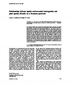
Temperature (°C)

35

(A)

Water temperature

30

25

20 Shallow Deep

15

Secchi disc depth (m)

5

(B)

Wet

Dry

Water clarity

4 3

RESULTS Environmental variables While, as demonstrated by ANOVA, water temperature differed significantly between dry and wet seasons and among locations (both p < 0.001) and between water depths (p < 0.05), there were significant interactions for location × depth, location × season and depth × season for this variable. The mean square values emphasized, however, that temperature was more strongly related to season (9.8) than either location (0.32) or water depth (0.005), and that season and location had a far greater influence on temperature than the interactions. At each location, water temperatures in both depths were far greater during the wet than dry seasons (Fig. 2A). Although water temperatures at the more northern locations were similar in deep and shallow waters in the wet and dry seasons, they increasingly diverged with depth in a southwards direction during both seasons, but with those for shallow water becoming greatest in the wet and those for deep water becoming greatest in the dry. These differences account for the interactions between location, depth and season. The mean depth of water clarity differed significantly among locations (p < 0.001) and between seasons (p < 0.05), but not between water depths (p > 0.05), and there were no significant interactions between these variables (p > 0.05). Water clarity was related more to location (mean square = 1.10) than season (mean square = 0.09). Water clarity was least at Cape Voltaire and Hall Point in the north (~1.7 m) and greatest at Locker Point in the south (Fig. 2B). Although water clarity was very similar in the wet and dry seasons at the 2 most northern locations (Cape Voltaire and Hall Point), it was greater during the dry season at the other 5 locations and particularly at the 2 most southern locations (Cape Preston and Locker Point).

2

Dominant species and families

1

Dry season Wet season

0

n

t

in Po

n re ud

to

ra

ut

ss

t in

Po

es Pr

er

ck

e ap

Lo

C Ke

Bo

u

nt

ire

lta Vo

ia

e

ap

e ap

C

C

er

e

oi lP

al

Em

H

ap C

Fig. 2. Mean values (± 95% CI) for (A) water temperatures and (B) water clarity depths at each of the 7 sampling locations in tropical north-western Australia. Note error bars are too small in the first plot to be effectively illustrated

Trawling in deep and shallow inshore waters at the 7 locations along the NWA coast in 2001 and 2002 yielded 84 781 fishes, which represented 272 species of teleost belonging to 167 genera and 74 families (Table 1). None of the 13 elasmobranch species, representing 9 genera and 6 families, was abundant or regularly caught. Certain species showed a pronounced tendency to occur either exclusively or predominantly in certain

Leiognathus splendens 16354 19.3 Terapon theraps 9041 10.7 Secutor insidiator 8284 9.8 Selaroides leptolepis 5070 6.0 Leiognathus leuciscus 4484 5.3 Upeneus sulphureus 4380 5.2 Saurida spp. 3079 3.6 Pristotis obtusirostris 3068 3.6 Carangoides malabaricus 2705 3.2 Paramonacanthus 2505 3.0 choirocephalus Caranx bucculentus 2411 2.8 Lethrinus genivittatus 1586 1.9 Saurida tumbil 1074 1.3 Pomadasys maculatum 998 1.2 Torquigener pallimaculatus 877 1.0 Upeneus asymmetricus 768 0.9 Leiognathus equulus 728 0.9 Secutor interruptus 726 0.9 Leiognathus fasciatus 613 0.7 Engyprosopon grandisquama 527 0.6 Leiognathus bindus 473 0.6 Engyprosopon maldiviensis 465 0.5 Siganus fuscescens 445 0.5 Gerres filamentosus 423 0.5 Choerodon cephalotes 418 0.5 Johnius borneensis 388 0.5 Parapercis nebulosa 386 0.5 Pentapodus porosus 384 0.5 Sillago ingenuua 376 0.4 Apogon unitaeniatus 373 0.4 Nemipterus furcosus 372 0.4 Leiognathus decorus 350 0.4 Apogon fasciatus 319 0.4 Total numbers 84781 Total biomass (kg) Mean overall density 298 (0.01 km–2) Mean overall biomass (kg 0.01 km–2) Number of species 285

Species

4.7 1.9 4.0 1.8 0.6 0.8 0.9 0.1 0.6 0.3 0.1 0.4 0.7 0.6 2.3 0.4 0.9 1.0 0.7 0.1 0.7 0.3 0.1

96 39 82 38 12 16 19 2 13 6 2 9 14 12 47 8 17 21 14 3 15 5 3

19

2047

8.2 9.8 3.2 5.8 2.9 3.7 7.9 1.7 1.5 1.6

168 201 65 119 60 76 161 34 31 33

Numbers Biomass N (%) B (%)

5 16

3

2 21

2

2

1

3

32 75 97 140 419 28 13 2 14 1 4

5

46

0

16

2