Memory & Cognition 2002, 30 (1), 138-149
Relative informativeness of quantifiers used in syllogistic reasoning MIKE OAKSFORD and LISA ROBERTS Cardiff University, Cardiff, Wales and NICK CHATER University of Warwick, Coventry, England Three experiments tested a possible resolution of the probability heuristics model (PHM) of syllogistic reasoning proposed by Chater and Oaksford (1999), with their experimental results apparently showing that the generalized quantifier few was not as informative as suggested theoretically. Modifying the interpretation of few to take into account the distinction between positive and negative quantifiers (Moxey & Sanford, 1993) indicated two orderings over the quantifiers all, most, few, some, none, and some. . .not that are more consistent with the results. Experiments 1–3 tested these orderings empirically by having participants rank whether a quantifier applied to a particular probabilistic state of affairs. Experiments 1 and 2 showed that participants agreed on when a quantifier applied and that the empirically derived informativeness orderings were consistent with the proposed modifications of the order. Experiment 3 showed that this finding was robust even when response competition was eliminated.
Over the last few years, we have been developing a probabilistic approach to deductive reasoning (for overviews, see Chater & Oaksford, 2000, 2001; Eysenck & Keane, 2000; Manktelow, 1999; Oaksford & Chater, 2001). We recently have extended this approach to syllogisms (Chater & Oaksford, 1999)—that is, to inferences that combine two quantified (all, some, some. . .not, or none) premises to form inferences such as, All Y are X, Some Y are Z, therefore, Some X are Z. Oaksford and Chater (1994, 1996, 1998) argued that people make errors on logical reasoning tasks because they generalize their everyday probabilistic reasoning strategies to the laboratory. Substantiating this claim involved showing that the probabilistic account could apply to an unquestionably logical task. Although syllogisms arguably play only a minor role in everyday reasoning, they do fit this bill. They have also been used as the major testing ground for theories of reasoning (e.g., Bucciarelli & JohnsonLaird, 1999; Evans, Handley, Harper, & Johnson-Laird, 1999; Guyote & Sternberg, 1981; Johnson-Laird, 1983; Newstead, Handley, & Buck, 1999; Polk & Newell, 1995; Rips, 1994). Chater and Oaksford’s (1999) probability heuristics model (PHM) explains the standard pattern of inferences using the logical quantifiers. Importantly, they also showed that it generalizes to syllogistic reasoning involving the Correspondence should be addressed to M. Oaksford, School of Psychology, Cardiff University, P. O. Box 901, Cardiff, CF10 3YG, U.K. (e-mail:
[email protected]). —Accepted by previous editorial team
Copyright 2002 Psychonomic Society, Inc.
generalized quantifiers most and few (Barwise & Cooper, 1981). Other theories of reasoning have not been applied to these quantifiers (although see Johnson-Laird, 1983, 1994, for discussion of how they might be represented in mental models theory). We would argue that explaining syllogistic reasoning with generalized quantifiers is the main testing ground for distinguishing between theories in this area. The variety of quantifiers that figure in natural language goes far beyond the logical quantifiers (e.g., Moxey & Sanford, 1993), and people seem to find reasoning with them natural (Chater & Oaksford, 1999). Therefore constraining theories to just the four logical quantifiers seems overly restrictive from a psychological point of view. Some of Chater and Oaksford’s (1999) results, however, were unexpected and questioned a core assumption of PHM concerning the ordering in the informativeness of the quantifiers (see below). Problems arose mainly for few. The goal of the work reported here is to show that these results can be explained by the pragmatics of this quantifier. Importantly, PHM can incorporate these pragmatic phenomena, and this leads to a change in the informativeness order. This change allows PHM to explain Chater and Oaksford’s (1999) anomalous results. In this paper we report experiments testing this explanation. The Probability Heuristics Model In PHM (Chater & Oaksford, 1999), participants reason syllogistically by applying various heuristics. How they are applied depends on an informativeness ordering over the quantifiers. For example, it is more informative to know that All the customers are vegetarians than that
138
INFORMATIVENESS OF QUANTIFIERS Some of the customers are not vegetarians. This is because the all statement is much less likely to be true. The overall ordering in informativeness exploited in PHM was all . most . few . some . none . some. . .not. The heuristics operate over a representation of the premises to generate a representation of the putative conclusion. Take the example just given, All Y are X, Some Y are Z, therefore, Some X are Z. (X refers to the end term of the first premise and Z to the end term of the second premise. Y is the middle term that connects the two premises.) The most important heuristic is the “minheuristic,” which advises selecting the form of the least informative premise as the form of the conclusion: Some _ are _, where underscores (“_”) act as placeholders for the end terms (X or Z ). Other heuristics determine the order of end terms in the conclusion, and confidence that the conclusion is valid. The min-heuristic and the other heuristics depend on the informativeness ordering that Chater and Oaksford (1999) derived theoretically. Two experiments combining the generalized quantifiers most and few with the logical quantifiers were generally supportive of PHM. However, there were some anomalies. For example, according to the informativeness order, for syllogisms in which the two premises are few and some. . .not, the minheuristic predicts a some. . .not conclusion. However, in Chater and Oaksford’s (1999) Experiment 1, there was no significant difference in the frequency of endorsing few and some. . .not, although they were both endorsed significantly more often than the other possible response options. Moreover, for syllogisms in which the two premises are few and some, the min-heuristic predicts a some conclusion. However, in Chater and Oaksford’s (1999) Experiment 2 there was no significant difference in the frequency of endorsing few and some, although the trend was for more endorsements of few. Both were endorsed significantly more often than the other possible response options. These results suggest that in Chater and Oaksford’s (1999) Experiment 1, few was regarded as being only as informative as some. . .not, whereas in their Experiment 2, few was regarded as being as informative as, or perhaps less informative than, some. Some Pragmatic Properties of the Quantifiers Why should this happen? We think two factors are involved. The first is an ambiguity in the interpretation of few. The second suggests that one interpretation of few was adopted in one experiment but the other interpretation was adopted in the other experiment. There is a pragmatic distinction between positive and negative quantifiers (Moxey & Sanford, 1987, 1993; Paterson, Sanford, Moxey, & Dawydiak, 1998; Sanford, Moxey, & Paterson, 1994, 1996). A positive quantifier implies that the corresponding all statement is false. So, for example, Some staff attended the meeting suggests that it is false that All staff attended the meeting, al-
139
though this does not follow logically. This implicature can be suspended using the phrase “if not all” (Horn, 1989; Moxey & Sanford, 1993): Some staff attended the meeting, if not all. Some is a positive quantifier, as is most (as a similar check readily demonstrates). A negative quantifier implicates the falsity of the corresponding none statement. For example, Some staff did not attend the meeting, if not all, means that it is possible that All staff did not attend, which is synonymous with None of the staff attended. That is, the implicature of some. . .not is that not none of the staff attended the meeting. Therefore, Some X are not Y is a negative quantifier. Distinguishing positive from negative quantifiers reveals an epistemological ambiguity in their interpretation. For example, someone may assert that Some staff attended the meeting because all of the staff they know about attended, but they do not know if the other staff members attended. Here some allows the possibility that All X are Y. However, someone may assert this because some of the staff members they know about attended and some did not attend. Here some implicates the falsity of All X are Y. Resolving this ambiguity requires more information from one’s interlocuter, information that is not available in a laboratory reasoning task. Therefore, it is reasonable to assume that many participants interpret some and some. . .not as allowing the possibility of all and none, respectively. This interpretation is captured in Chater and Oaksford’s (1999) probabilistic semantics, where the meaning of a quantified statement, having subject term X and predicate term Y, is given by the conditional probability of Y given X (P(Y | X )). On this account, all means that P(Y | X ) 5 1, none means that P(Y | X ) 5 0, some means that P(Y | X ) . 0, and some. . .not means that P(Y | X) , 1. That is, the probability interval for some includes that for all and the probability interval for some. . .not includes that for none. Because most is a positive quantifier, Chater and Oaksford (1999) should have allowed the possibility of all. This is achieved by letting most mean that P(Y | X ) . 1 2 D (where D is small) rather than 1 . P(Y | X ) . 1 2 D. Whether few is a positive or negative quantifier may be crucial to explaining the apparent inferential changes between Chater and Oaksford’s (1999) experiments. Interpreting this quantifier may be ambiguous because although few is a negative quantifier, a few is a positive quantifier. According to Chater and Oaksford’s (1999) original semantics, the meaning of few is that 0 , P(Y | X ) , D. By analogy with most, changing this semantics to include none simply means changing this definition to P(Y | X ) , D. We will refer to this quantifier as few2. How should we cope probabilistically with a few? A few can apply to the same region that we initially assigned to few. Someone may assert that Few staff (X) attended the meeting (Y), if not none because all of the, perhaps large, sample of staff (say, 90 out of a total of 100) they know about did not. Therefore, P(Y | X ) could
140
OAKSFORD, ROBERTS, AND CHATER
be as low as 0 but only as high as .1. Consistent with the sample, however, confidence should be biased toward the low end of this range (i.e., toward none). In contrast, someone may assert that A few staff attended the meeting, if not all because all of the, very small, sample of staff (say, 2) they know about did attend. Therefore P(Y | X ) could be as high as 1 but as low as .02. Consistent with their sample, however, confidence should be biased toward the high end of this range—that is, toward most and all. This seems consistent with the acceptability of the other quantifiers as suspenders of implicature: A few staff attended the meeting, if not all. A few staff attended the meeting, if not most. *A few staff attended the meeting, if not none. *A few staff attended the meeting, if not some. *A few staff attended the meeting, if all did. (* indicates pragmatic infelicity) (The final example is an attempt to make more sense of . . ., if not some did not. It is not the case that someone did not attend is equivalent to everyone attended.) Consequently, A few X are Y must allow the possibility that All X are Y and that Most X are Y, but not any of the other possibilities described by the remaining quantifiers. We therefore interpret A few X are Y to mean that the probability of Y given X can take on values between 0 and D and between 1 2 D and 1. We will refer to a few interpreted in this way as few1. Of course the expression a few was not used in Chater and Oaksford’s (1999) experiments. However, we argue that when interpreting the decontextualized statements of a syllogistic reasoning experiment (e.g., Few artists are beekeepers), both possible interpretations may be considered. The second factor that may explain the anomalies in Chater and Oaksford’s (1999) experiments concerns why
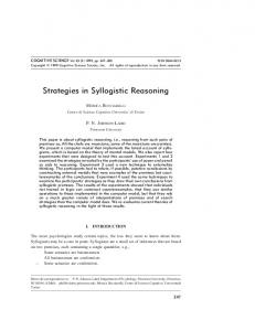
Figure 1. Schematic diagram of the frequency of true statements as a function of P(Y | X ). The frequency of none (E) statements (which is over half of all statements) is represented by the filled arrow. The frequency of all (A) statements is represented by the small square filled box. The frequencies of the few (F) and most (M) statements are given by the areas marked in white. The remaining shaded area, Z, does not correspond directly to any particular quantifier.
these different interpretations have been adopted in each experiment. The appropriateness of a quantifier may depend on the other quantifiers available (Brownell & Caramazza, 1978; Moxey & Sanford, 1993). For example, suppose that 10 out of 100 squares are white. One might choose to describe this state of affairs as Few squares are white. But if few was unavailable, then Some squares are white may do perfectly well. In Chater and Oaksford (1999), only the quantifiers all, most, few, and some. . .not were used in Experiment 1, and only the quantifiers most, few, some, and none were used in Experiment 2. This was to keep the total number of syllogisms in a single experiment at manageable levels. In Chater and Oaksford’s (1999) experiments, we suspect that the change in the quantifiers used has led participants to interpret “few” as few2 in Experiment 1 and as few1 in Experiment 2. This is because in Experiment 1, using all, most, few, and some. . .not, few is not needed to express the possibility of all or most because these quantifiers are available. Consequently “few” was interpreted as few2—that is, as applying only to the bottom end of the probability scale. The reverse was true for Experiment 2, which used most, few, some, and none. Here few is not needed to express none as this quantifier is available. Consequently, “few” was interpreted as few1—that is, as applying to the top end of the probability scale. Constructing an Informativeness Order There are several ways in which we could investigate this explanation of Chater and Oaksford’s (1999) results. In these experiments we investigated directly whether this interpretational change for few could explain the changes in its place in the informativeness order. If it can, then these results may be consistent with the minheuristic, the core of the PHM model. To see whether this is the case, we need to outline how an informativeness order is constructed. In Chater and Oaksford (1999), informativeness was calculated with respect to the probability density function shown in Figure 1. This shows the frequency of true statements as a function of P(Y | X). Taking any two terms at random, Chater and Oaksford (1999) argued that the highest density of true statements will correspond to P(Y | X ) values of zero. For example, the probability that a table is a toupee is zero, and so the only true statement that can be made using these two terms is that No toupees are tables. These will be most frequent because of the rarity assumption (Oaksford & Chater, 1994, 1996): Most terms apply only to a small number of objects and hence rarely cross-classify them. The large arrow at P(Y | X ) 5 0 (marked E) indicates that, for randomly selected terms, none statements are very frequently true— that is, more than half (.5) of the time. The area A corresponds to the probability that a true statement is made using all. In Chater and Oaksford’s (1999) original account, the areas marked M and F corresponded to the probability that a true statement is made using most
INFORMATIVENESS OF QUANTIFIERS [lower bound at P(Y | X ) 5 1 2 D] and few [upper bound at P(Y | X ) 5 D], respectively. The probabilities that true statements are made using some or some. . .not are sums over the other areas, some 5 F 1 Z 1 M 1 A, some. . . not 5 E 1 F 1 Z 1 M. To calculate informativeness, the probability of making a true statement is converted to bits of information using Shannon’s (Shannon & Weaver, 1949) surprisal formula. So the informativeness of a quantified statement Q is equal to log2[1/P(Q is true)]. Consequently, the lower the probability of making a true statement, the more informative it is. The probability densities in Figure 1 led to the informativeness order described earlier. The regions of the probability density function in Figure 1 can also illustrate how our new interpretations for the quantifiers affect the informativeness ordering. The changes affect most and few. Most is straightforward: Rather than just M, most now corresponds to the region M 1 A. Few1 corresponds to the area F 1 M 1 A. This means that the probabilities for few1 and some (F 1 Z 1 M 1 A) move much closer together. Moreover, as D increases toward .5, the area Z tends toward zero, at which point few1 and some would be equally informative, which was what Chater and Oaksford (1999) found in their Experiment 2. However, few2 corresponds to the area E 1 F. This means that although the probabilities for few2 and some. . .not (E 1 F 1 Z 1 M) move much closer together with increases in D (to a maximum of .5), this factor alone could not account for Chater and Oaksford’s (1999) finding that few2 and some. . .not seemed to be treated as equally informative in their Experiment 1. There are two unrealistic assumptions built in to these calculations of informativeness. First, D is the same for few and most, but there is no reason why this should be the case. Second, a quantifier (e.g., few) is as likely to be used to describe a state of affairs in one part of the interval it covers as another. So, for example, Few squares are white is as likely to be used to describe the situation where 1 out of a 100 squares is white as where 20 out of a 100 squares are white. This again seems unrealistic. Both of these assumptions are consequences of the intervalbased semantics assigned to the quantifiers; that is, the meaning of each quantifier is given a (possibly overlapping) interval on the P(Y | X ) scale. It is probably more realistic to take a distributional approach. That is, a quantifier will display a certain probability of being used that varies with P(Y | X ); D is then no longer a fixed point but is defined as the value of P(Y | X ), for which the probability of using few is negligible. What is required is a function relating P(Y | X ) to the probability of using each quantifier. This provides a “membership” function for each quantifier. There has been much work deriving these functions for a variety of quantified terms (e.g., Rapoport, Wallsten, & Cox, 1987; Wallsten, Budescu, Rapoport, Zwick, & Forsyth, 1986). These can then be combined with the probability density function in Figure 1 to obtain informativeness orderings.
141
That is, rather than assuming that the probability that a quantifier will be used in its interval is 1, we allow this probability to be determined by the membership function. This means that a term is more informative when it is unlikely to be used, and this seems intuitively correct. When a politician asserts that “most people voted ‘for’ in the referendum,” when only 52% did so, this is very informative about the politician’s attitudes. There have been many criticisms of the membership function approach to the meaning of the quantif iers (Moxey & Sanford, 1993). However, a probabilistic account does not have to provide the meaning of these terms. Rather, it can be regarded as providing their core meanings, which are used to reason syllogistically. Even if our account of quantifier meaning is incomplete, it is an empirical question whether we have captured enough of the meaning to explain syllogistic reasoning. One criticism of membership functions is that they are context sensitive (Moxey & Sanford, 1993). We have already appealed to one context effect: Whether a term is used to describe a state of affairs depends on the other terms available. In syllogistic reasoning experiments, the possible options are always restricted to the quantifiers used as premises. Chater and Oaksford’s (1999) theory has been applied only to the logical quantifiers and most and few. Consequently, to see if our account can explain Chater and Oaksford’s (1999) results, membership functions are required for the case where only these quantifiers are available. However, no existing experiments derived these functions for just these quantifiers. We therefore derived membership functions for these quantifiers to test our account of Chater and Oaksford’s (1999) results. We made three predictions regarding when these membership functions are combined with the probability density function in Figure 1 to derive informativeness orders. First, there should be significant differences in the informativeness of the quantifiers according to our theoretical ordering. Second, when “few” is interpreted as few1, there will be either no differences in informativeness between few and some, or some will be more informative than few. Third, when “few” is interpreted as few2, there will be no differences in informativeness between few and some. . .not. In these experiments we are predicting the absence of an effect. Consequently, following other researchers who have tested similar predictions (e.g., Kintsch, 1974, chap. 11; Manktelow & Evans, 1979), we conducted a sequence of experiments, each of which derived membership functions in a different way. EXPERIMENT 1 In this experiment, one group of participants was presented with verbal descriptions such as There are 50 squares of which 10 are white and another group with visual arrays displaying the same information. The statements and the arrays were varied in steps of .1 from 0 to
142
OAKSFORD, ROBERTS, AND CHATER
1 along the probability scale. Participants were then given all possible quantified descriptions of the described state of affairs (e.g., All the squares are white, Most of the squares are white . . ., etc.). They were then asked to select which quantifiers they thought applied to the state of affairs, rank-ordering them when they thought that more than one could apply. A visual presentation condition was included to determine whether membership functions were stable across different modes of presentation. It could also be argued that people are more familiar with assigning quantifiers to perceived or imagined states of affairs rather than to verbal descriptions. So the predicted null effects may arise in the verbal condition because of inaccuracies increasing the variance in the data. Previous research on membership functions sought to derive maximally discriminatory psychometric scales, and consequently each participant was asked to judge the applicability of the quantifiers many times (e.g., Rapoport et al., 1987; Wallsten et al., 1986). In contrast we asked participants for only one judgment at each value for P(Y | X ). This was primarily to reduce the time on task. We also used the ranking procedure just described, although in subsequent experiments we changed this procedure to see whether this would alter our results. This procedure was used because, as we have discussed, the context of the other quantifiers influences this judgment. We felt it would be easier to make the comparative judgment of whether one quantifier applied more than another using a ranking procedure rather than asking the participants to assign, say, a number between 1 and 100 to each quantifier. To compute the informativeness order, these ranks were converted to probabilities (see the Appendix). In past research, different participants sometimes provided different membership functions, which may have masked the effects we were looking for. Alternatively, they may only be present in the aggregate data, although two (or more) subsets of participants are doing something rather different. Individual differences in strategy have been observed in syllogistic reasoning (Bucciarelli & Johnson-Laird, 1999; Ford, 1994). However, we know of no reports of systematic differences between participants in interpretation. Nonetheless, in these experiments we checked that participants substantially agreed on which quantifiers applied at each level of P(Y | X ). Method
Participants. Eighty-one undergraduate psychology students at Cardiff University participated in return for course credit, 45 in the verbal presentation condition and 36 in the visual presentation condition. Materials. Each participant received a booklet containing a set of 11 scenarios, in different random orders. In each booklet, general instructions were given on the first page and an example on the second page. In the verbal condition, each state of affairs consisted of a statement such as In a room of 100 people, there are 50 artists of whom 15 are beekeepers . In the visual condition, participants viewed a 5 3 10 array of black-and-white squares. The proportion
of black squares was varied to achieve the probability manipulation. P(Y | X ) was varied throughout the experiment by varying the numbers of objects that fell into the relevant classes (0–50 at intervals of 5). There were always 50 people (squares) who could be described by the subject term (e.g., verbal condition: artists; visual condition: squares). The proportion that could also be described by the predicate term (e.g., verbal condition: beekeepers; visual condition: black) was varied. The lexical categories of the 11 statements in the verbal condition were different for each value of P(Y | X ). The response options involved the quantif iers all, most, some, some. . .not, few, and none, and the additional option “none of the above.” Procedure. Participants were tested individually. On entering the experimental room they were assigned randomly to either the verbal or visual condition. They were then seated in individual experimental cubicles where the materials were laid out face down on a table. When the booklet was turned over, the first page revealed the following instructions (in the visual condition, the text in italic was replaced with the text in parentheses): During the course of this experiment, you will be given a set of statements to read (presented with a series of illustrations). A list of options will then be given describing the situation illustrated in the previous set of statements (that describe the situation presented in the illustrations). We would like you to select the phrase that you think best describes the situation. If you decide to choose more than one option then please indicate your preference by using numbers, giving your first choice a value of 1, second choice a value of 2, and so on. An example is given on the following page.
After reading the instructions, participants were presented with each of the 11 scenarios in random order. They were told that there was no time limit (typically, they completed the task in under 15 min). For each scenario they were presented with the following statements (visual condition in parentheses): All of the artists (squares) are beekeepers (black) Most of the artists (squares) are beekeepers (black) Some of the artists (squares) are beekeepers (black) Some of the artists (squares) are not beekeepers (black) Few of the artists (squares) are beekeepers (black) None of the artists (squares) are beekeepers (black) None of the above
When a participant had finished the booklet, they were thanked for their participation and were debriefed concerning the purpose of the experiment.
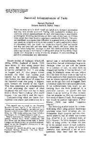
Results and Discussion Figure 2 shows the membership functions for the verbal and visual conditions, respectively. The inclusion ratings have been rescaled to the 0–1 interval (by inverting and dividing by 6). Each point shows the mean rating for each quantifier. Each function is only shown within the limits where it was used to describe the probabilistic relation between X and Y. Outside these limits, the chance of being used was not significantly greater than 0 in onesample t tests. So, for example, from Figure 2, it can be seen that F was used only in the interval .1 # P(Y | X ) # .4. Within these limits, we tested for any differences between the verbal and visual conditions using two-way mixed analyses of variance (ANOVAs) with condition as the between-subjects factor and P(Y | X ) as the withinsubjects factor. All and none were excluded because, in both conditions, they were used only when P(Y | X ) was 1 or 0, respectively. For few there was no main effect of condition and no interaction. For most there was no main
INFORMATIVENESS OF QUANTIFIERS
143
Figure 2. Membership functions for the verbal and visual conditions in Experiment 1, showing mean probability of inclusion as a function of P(Y | X ) for the quantifiers all, most, some (filled markers) and few, none, and some. . .not (unfilled markers). The top panel shows the verbal condition and the bottom panel shows the visual condition.
effect of condition but there was a significant interaction [F(5,395) 5 4.78, MS e 5 2.82, p , .0005]. Differences were found only in the mid-range when P(Y | X) 5 .4 or .5. At these values most was ranked more highly in the visual condition than in the verbal condition. Around the midrange it seems harder to make the perceptual discrimination that there are more black than white squares. For some a main effect of condition was modified by a significant interaction [F(8,632) 5 2.16, MSe 5 3.31, p , .05]. Some was ranked more highly in the verbal than in the visual condition, but primarily in the midrange from P(Y | X ) 5 .4 to .7. Here the use of some seems to fall off much more steeply as P(Y | X ) increases in the vi-
sual condition than in the verbal condition. A main effect was found for some. . .not [F(1,79) 5 4.47, MSe 5 23.80, p , .05], but with no interaction. Some. . .not was ranked more highly in the verbal than in the visual condition. These are interesting differences that deserve investigation in their own right. However, we offer no explanation for them here. The critical question is, despite these differences between conditions, do participants largely agree on which quantifiers apply at each level of P(Y | X )? Participants ranked which quantifiers applied at each value of P(Y | X ). Consequently we calculated agreement at each of the 11 values of P(Y | X ) using Kendall’s coefficient of concordance (Siegal & Castellan, 1988, pp. 262–
144
OAKSFORD, ROBERTS, AND CHATER
272). Across conditions, the mean coefficient of concordance, W(N 5 6, k 5 81), was .72 (SD 5 .12). At every value of P(Y | X ), this coefficient was greater than .53, indicating that there was significantly greater agreement among the participants than would be expected by chance: All values of W(N 5 6, k 5 81) were significant at least at the .0001 level (assessed against the c 2 distribution; see Siegel & Castellan, 1988, p. 269). Consequently, in this experiment participants seemed to agree on the order in which these six quantifiers apply to a probabilistically defined state of affairs whether it was presented visually or described verbally. Informally, informativeness was calculated using the probability that a quantifier is used to make a true statement (see the Appendix for the formal derivation). The lower this probability, the more informative the statement. This probability is calculated by multiplying the probability with which a quantifier is used at a given value of P(Y | X ) (given by the membership function) by the probability that it is true at that value (given by Figure 1). This resulted in an informativeness order for each participant, allowing statistical testing of our predictions. We collapsed across conditions because participants agreed on when a quantifier applied. Moreover, because we predicted no differences, the increased statistical power provided a stronger test of our hypothesis. For each of the experiments reported here, Table 1 shows the mean informativeness in bits of each quantifier once their negative or positive status is taken into account, as outlined in the introduction. For all three experiments, we conducted two one-way ANOVAs, one with “few” interpreted as few – and one with “few” interpreted as few1. We then conducted pairwise comparisons by using either Scheffé tests or t tests. The Scheffé tests were to confirm that differences were present when they were predicted to be (so maximum protection against conducting multiple tests is required), and the t tests were used to confirm that effects did not exist when they were predicted not to. When interpreting “few” as few2, although all other pairwise comparisons were significant, there was no significant difference in informativeness between few2 and some. . .not. When interpreting “few” as few1, although all other pairwise comparisons were significant, there was no significant difference in informativeness between few1 and some. These results confirm the predictions outlined in the introduction. The apparent changes in the position of
“few” in the informativeness order between Chater and Oaksford’s (1999) two experiments may be because “few” can be interpreted as either a positive or a negative quantifier. EXPERIMENT 2 Because of the possibility of individual differences, it is important to the validity of these experiments that participants substantially agree on the quantifiers that apply in each probabilistic state of affairs. The ranking procedure we used in Experiment 1 tends to lead to many ties. This is because most participants only rank one or two quantifiers as applying to a given state of affairs and so the rest are ranked 0. In computing Kendall’s coefficient of concordance, a correction is applied to deal with ties (Siegal & Castellan, 1988, pp. 266-269). This correction increases the coefficient of concordance. If there are many ties, as in these experiments, the correction can inflate the value of W. In Experiment 2, we therefore had participants rank all the quantifiers, so that a unique rank was assigned to each quantifier, thus avoiding the need to apply a correction. Given that at many values of P(Y | X ) most quantifiers were assigned the same rank (i.e., 0, in Experiment 1), this procedure may increase the chances of disagreement. If these quantifiers are regarded as unlikely to apply with equal probability, then their rank may be assigned randomly in this experiment. One consequence of this procedure was to force participants to provide rankings for all and none at P(Y | X ) values between 0 and 1. However, in Experiment 1, participants never used these quantifiers at these intermediate values. Calculating informativeness would be considerably distorted if we included the intermediate rankings for all and none. Consequently, in calculating informativeness, all and none were treated as applying only when P(Y | X ) 5 1 or 0, respectively, and no other quantifier was treated as applying at these values. Method
Particip ants. Forty undergraduate psychology students at Cardiff University received course credit for participating in this experiment. Materials. The booklets were the same as those used in Experiment 1 (verbal condition) except that the participants in this experiment were asked to rank-order all six quantif iers. Procedure. The procedure was identical to that in Experiment 1, except for the necessary adjustments to the instructions. The third
Table 1 Mean Informativeness and Standard Deviations in Bits of the Quantifiers all, most, few 2 , few 1 , some, none, and some . . .not in Experiments 1 (N = 81), 2 (N = 40), and 3 (N = 50), Calculated as in the Appendix Quantifiers
_
all
_
most
_
few2
_
few 1
_
some
_
none
some. . .not
_
Experiment
m
SD
m
SD
m
SD
m
SD
m
SD
m
SD
m
SD
1 2 3
6.09 6.15 6.59
.35 .05 .94
4.18 3.61 4.53
.60 .18 .62
.65 .58 .79
.24 .02 .41
2.61 2.48 2.50
.53 .10 .58
2.60 2.92 2.76
.57 .12 .35
.96 .81 1.27
.45 .00 .69
.63 .59 .62
.24 .03 .28
INFORMATIVENESS OF QUANTIFIERS
145
Figure 3. Membership functions in Experiment 2, showing mean inclusion ratings as a function of P(Y| X) for the quantifiers all, most, some (filled markers) and few, none, and some...not (unfilled markers).
and fourth sentences were replaced with the following: “We would like you to rank these options in terms of how appropriate you think they are for describing the situation. Please indicate your preference by using numbers, giving your first choice a value of 1, second choice a value of 2, and so on.”
Results and Discussion Figure 3 shows the membership functions for Experiment 2. At every value of P(Y | X ), there was significantly greater agreement among the 40 participants than would be expected by chance: All values of W(N 5 6, k 5 40) were greater than .79, which meant that all were significant at least at the .0001 level. The mean was .84 (SD 5 .04). Unexpectedly, even without a correction for ties, agreement on which quantifiers applied increased considerably. Consequently, the excellent agreement found in Experiment 1 was not the product of correcting for the large number of ties. The coefficient of concordance is an index of lack of variation in participants’ responses; thus the higher this coefficient, the lower the variance. In computing the informativeness of each quantifier, the only variation is provided by the membership functions because the conversion to bits (see the Appendix) involves exactly the same transformation for each participant’s data. Therefore the increases in agreement we observed should translate into much lower variances in the informativeness of each quantifier. Table 1 shows that this was the case: The standard deviations were all a lot lower than in Experiment 1. Despite this reduction in the variance, for interpretations of “few” as few2, although all other pairwise comparisons were significant, there was no significant difference in informativeness between few2 and some. . .not. However, for interpretations of “few” as few1, all other pairwise comparisons were significant
and a significant difference in informativeness between few1 and some was observed. This finding is consistent with Chater and Oaksford’s (1999) results of a close to significant trend such that few was selected more than some. This in turn is consistent with the min-heuristic if some is interpreted as more informative than few, as in Chater and Oaksford’s (1999) Experiment 2. EXPERIMENT 3 There were two reasons for conducting Experiment 3. First, we wanted to determine how robust these findings were. In particular we wondered whether the informativeness order would stand up when the quantifiers were not in direct response competition. Thus, in this experiment we removed the competitive element by having participants give a binary response as to whether a quantifier, presented on its own, applied to a probabilistic state of affairs. This also allowed us to plot the probability that a quantifier can be used at a given value of P(Y | X ). Our hunch was that in these circumstances, which remove the context effects discussed in the introduction, people would endorse a quantifier across its whole range of applicability. Second, in Experiments 1 and 2, we only checked for agreement between participants at each value of P(Y | X ) because participants ranked the six quantifiers at each of these values. However, participants did not rank each value for a particular quantifier, so we could not test agreement for each quantifier. Could we have used the rankings we did obtain to calculate this? This was not feasible because the large number of ties (11 categories but only a maximum of 6 ranks) can lead to the correction term dominating the calculation of W. With binary
146
OAKSFORD, ROBERTS, AND CHATER
data we used the average chi-square as an index of agreement. For each quantifier, at each value of P(Y | X ), if participants select a quantif ier at random, then half will select it and half will not. Significant deviation from this distribution shows significantly above-chance agreement. Method
Participants. Fifty undergraduate psychology students at Cardiff University received course credit for participating in this experiment. Design. In this experiment participants were presented with the same verbally presented situations as in Experiments 1 and 2, but now with only one quantifier on each trial, making 66 trials overall. The materials were the same as those used in Experiment 1. Procedure. This experiment was presented on computer using the PsyScope software (Cohen, MacWhinney, Flatt, & Provost, 1993) to control the presentation of stimuli and to record responses. The instructions were similar to those in Experiments 1 and 2. Participants pressed a “yes” (“Z”) button if they thought the statement was a good description and a “no” (“M”) button if they did not think that the statement was a good description.
Results and Discussion Figure 4 shows the membership functions for Experiment 3; we assessed differences from 0 using one-sample sign tests. For each quantifier, we tested whether there were more participants agreeing on whether it applied than would be expected by chance at each level of P(Y | X ) using the c 2 test. For all, the average c2(1) was 46.18 (SD 5 4.46), and at every value of P(Y | X ), c 2(1) was significant (. 38.72, p , .0001). For most, the average
c 2 (1) was 36.41 (SD 5 13.02), and at all values of P(Y | X ), c 2(1) was significant (. 23.12, p , .0001) except for P(Y | X ) 5 1. For few, the average c 2(1) was 33.86 (SD 5 14.46), and at all values of P(Y | X ), c 2(1) was significant (. 18, p , .0001) except for P(Y | X ) 5 .4. For some, the average c 2(1) was 30.69 (SD 5 11.95), and at all values of P(Y | X ), c 2(1) was significant (. 5.12, p , .05). For none, the average c 2(1) was 47.01 (SD 5 6.28), and at all values of P(Y | X), c 2(1) was significant (. 28.88, p , .0001). For some. . .not, the average c 2(1) was 34.07 (SD 5 11.41), and at all values of P(Y | X ), c 2(1) was significant (. 8, p , .005). Agreement failed to get abovechance levels for only 2 out of the 66 comparisons: for few when P(Y | X ) 5 .4 and for most when P(Y | X ) 5 1. Consequently, participants substantially agreed on whether a quantifier could be used to describe a particular probabilistic state of affairs. The informativeness order data in Table 1 were analyzed in the same way as in Experiment 1. When interpreting “few” as few2, although all other pairwise comparisons were significant, there was no significant difference in informativeness between few2 and some. . .not. For interpretations of “few” as few1, although all other pairwise comparisons were significant, there was no significant difference in informativeness between few1 and some. Thus in Experiment 3, where participants made independent judgments of applicability, uninfluenced by the other quantifiers, they nonetheless showed the same behavior as in Experiments 1 and 2. This would appear to indicate that although context effects may explain why
Figure 4. Membership functions in Experiment 3, showing the proportion of participants endorsing a quantifier as a function of P(Y | X ) for the quantifiers all, most, some (filled markers) and the quantifiers few, none, and some...not (unfilled markers). There are many values of P(Y | X ) for which some quantifiers take on the same values. When this happens, the unfilled marker is in the foreground. This happens for some and some...not between .2 and .5 (some...not was not endorsed at 1.0 and some was not endorsed at 0), and for most and few at .5 (most was not endorsed below .5).
INFORMATIVENESS OF QUANTIFIERS different interpretations of “few” were adopted in Chater and Oaksford’s (1999) experiments, people’s assessment of informativeness once these interpretations are adopted is independent of context. GENERAL DISCUSSIO N The purpose of these experiments was to test whether people’s assessment of when all, most, some, few, none, and some. . .not apply to a probabilistic state of affairs could explain the anomalous results found by Chater and Oaksford (1999). We argued that the pragmatic distinction between positive and negative quantifiers (e.g., Moxey & Sanford, 1993) suggested a possible ambiguity in the interpretation of few that may explain why it was treated as having the same informativeness as some in one of Chater and Oaksford’s (1999) experiments, but as having the same informativeness as some. . .not in the other. When this distinction was incorporated into their probabilistic interpretation of the quantifiers, the theoretical informativeness ordering came closer to that apparently revealed by Chater and Oaksford’s (1999) anomalous results. However, to test this explanation meant adopting a distributional- rather than an interval-based approach to the meaning of the quantifiers. The nature of these distributions was derived empirically in Experiments 1–3 by constructing membership functions. In Experiment 1, participants ranked the quantifiers for whether they applied to a range of verbally or visually presented probabilistic states of affairs. Consistent with our explanation of Chater and Oaksford’s (1999) results, there were no differences in informativeness between few1 and some, nor between few – and some. . .not. Because individual differences have been observed in membership functions, it was important to demonstrate that participants agreed on which quantifier applied. In Experiment 2, to avoid a possible criticism concerning the computation of Kendall’s coefficient of concordance, we had participants provide a unique ranking for each quantifier. Agreement was even higher than in Experiment 1. This radically reduced the variance, making a very strong test. Experiment 2 replicated the lack of an effect for few2 and some. . .not but not for few 1 and some. However, the direction of the effect—some was more informative than few1—was consistent with the trend in Chater and Oaksford’s (1999) results and with the min-heuristic. Experiment 3 tested the robustness of the informativeness order when the context provided by the other quantifiers is absent. The results replicated those from Experiment 1 and 2, suggesting that such a context does not generally affect people’s assessment of informativeness. In three experiments deriving informativeness orderings for the quantifiers used in Chater and Oaksford’s (1999) experiments, we found no differences in informativeness between few1 and some (with the exception of Experiment 2), or between few 2 and some. . .not. These findings therefore confirm our explanation of the
147
apparent anomalies found in Chater and Oaksford’s (1999) results. It could be argued that these experiments question the viability of PHM because we have derived informativeness orders empirically rather than formally. This might be thought to have the following consequences. First, it would appear to threaten our claim that people are rational because we derive our predictions from a purely formal model (Chater & Oaksford, 2000). Second, it threatens the testability of the model because there is no prior index of informativeness. However, our probabilistic models are rational because they show that people’s inferential behavior may be well adapted to the environment. For example, calculating the ordering theoretically (see Chater & Oaksford, 1999, Appendix A) involved making a rarity assumption; that is, the subject (X ) and predicate (Y ) terms describe rarely occurring properties in the world (see also Oaksford & Chater, 1994). An experiment where rarity was manipulated would be expected to alter the informativeness ordering in predictable ways. Similarly, we assumed an interval-based semantics in those calculations. Here we adopted a distributional approach and set those distributions empirically via the membership functions. The goal of any semantic theory, formal or otherwise, is to capture how people use their language, and this can only be determined empirically. Testability is also not in doubt. To predict the informativeness order, we need to know the range of quantifiers in play and their contextual effects based on a wellspecified pragmatic theory. The work of Moxey and Sanford (1993) is beginning to provide just this. We have been able to incorporate some of their pragmatic distinctions into our probabilistic model, allowing us to formally derive their consequences for the informational ordering. Then a prior index of informativeness can be derived from experiments like those reported here. Moreover, in testing theories, this is no different from any other area of science. Even in physics the fundamental constants of the theory (e.g., Planck’s constant) have to be determined empirically before the theory can support any predictions. The results of these experiments may appear narrowly focused on resolving just one anomaly for just one particular theory of syllogistic reasoning, with no further ramifications for which theory of syllogistic reasoning is correct. However, we think clear conclusions can be drawn from this work. Most obviously, if we had left this anomaly unexplained, other theoreticians would have correctly identified it as a problem that counts against the PHM. Therefore, to the extent that these experiments succeed in plugging that hole, they are supportive of PHM over other theories. More generally, this work raises the issue of when quantifiers, especially generalized quantifiers, can be used to describe a state of affairs. This may raise a problem for our account because it appears to rely on the idea that quantifiers identify well-def ined regions of the
148
OAKSFORD, ROBERTS, AND CHATER
probability scale, an idea thoroughly discredited by Moxey and Sanford (1993). They observed that for many generalized quantifiers there is no discrimination along the probability scale; that is, there are large areas of overlap. Any discrimination, they argued, is due to participants making comparative judgments (as in Experiments 1 and 2). In experiments using independent judgments (as in Experiment 3), many quantif iers cannot be discriminated. Consequently the reason for their use on particular occasions cannot be because they identify a particular range of probability values. However, consistent with Moxey and Sanford’s observations, PHM already allows a great deal of overlap between the quantifiers. The ordering over which our heuristics are defined depends on informativeness, not on the probability scale. And informativeness is calculated across the whole probability scale for each quantifier. Moxey and Sanford’s (1993) point, however, that quantifier selection must depend on more than the probability scale, is well taken. In our account of syllogistic reasoning, the min-heuristic selects the conclusion quantifier from those in the premises, and this seems to agree with the empirical evidence. However, the multiplicity of quantifiers that can apply to a given state of affairs may provide problems for theories, like mental models, that rely on mentally representing such states of affairs and “reading off ” appropriate conclusions. The problem is that just having a representation of the probabilistic relation between the end terms does not tell you which conclusion to draw. For example, the following mental model for Some X are Y, Some Y are Z: X
X
X Y
X Y Z
Y Z
Y Z
Z
Z
is consistent with the conclusions Few X are Z, Few Z are X, Some X are Z, and Some Z are not X (or Some X are not Z ). One might argue that some of these conclusions will be ruled out in the search for counter models. However, the recent evidence is that people only construct a single mental model (e.g., Evans et al., 1999; Newstead et al., 1999). Thus it is important for mental models that the most frequently occurring response is true in this model. However, the most frequent response to the Some X are Y, Some Y are Z syllogism is Some X are Z (60% in Chater & Oaksford’s, 1999, Experiment 2). This conclusion is true in the illustrated mental model, which makes it the best candidate for the single model of these premises that people initially construct. In which case, it is unclear why the Some X are Z response dominates over the other possible responses. Until mental models are extended to syllogistic reasoning with generalized quantifiers, it is unclear what principles will be invoked to resolve this ambiguity. In contrast, the min-heuristic unambiguously predicts a some conclusion, which is the probabilistically valid conclusion endorsed by most participants (Chater & Oaksford, 1999).
In conclusion, closer consideration of the pragmatics of quantified claims has allowed us to offer more detailed accounts of the data on syllogistic reasoning with generalized quantifiers. Some of Chater and Oaksford’s (1999) results that seemed at odds with their theoretical informativeness order are consistent with the orderings suggested by the distinction between positive and negative quantifiers. Consequently, understanding syllogistic reasoning performance will require close attention to the pragmatics of these statements. The main advantage of the probabilistic approach is that some of these pragmatic distinctions can be captured by a probabilistic semantics. It can therefore be shown directly how these pragmatic distinctions should alter people’s reasoning performance. REFERENCES Barwise, J., & Cooper, R. (1981). Generalized quantifiers and natural languages. Linguistics & Philosophy, 4, 159-219. Brownell, H. H., & Caramazza, A. (1978). Categorizing with overlapping categories. Memory & Cognition, 6, 481-490. Bucciarelli, M., & Johnson-Laird, P. N. (1999). Strategies in syllogistic reasoning. Cognitive Science, 23, 247-303. Chater, N., & Oaksford, M. (1999). The probability heuristics model of syllogistic reasoning. Cognitive Psychology, 38, 191-258. Chater, N., & Oaksford, M. (2000). The rational analysis of mind and behavior. Synthèse, 122, 93-131. Chater, N., & Oaksford, M. (2001). Human rationality and the psychology of reasoning: Where do we go from here? British Journal of Psychology, 92, 193-216. Cohen, J., MacWhinney, B., Flatt, M., & Provost, J. (1993). PsyScope: An interactive graphic system for designing and controlling experiments in the psychology laboratory using Macintosh computers. Behavior Research Methods, Instruments, & Computers, 25, 257-271. Evans, J. St. B. T., Handley, S. J., Harper, C. N. J., & JohnsonLaird, P. N. (1999). Reasoning about necessity and possibility: A test of the mental model theory of deduction. Journal of Experimental Psychology: Learning, Memory, & Cognition, 25, 1495-1513. Eysenck, M. W., & Keane, M. T. (2000). Cognitive psychology. Hove, U.K.: Psychology Press. Ford, M. (1994). Two modes of mental representation and problem solving in syllogistic reasoning. Cognition, 54, 1-71. Guyote, M. J., & Sternberg, R. J. (1981). A transitive chain theory of syllogistic reasoning. Cognitive Psychology, 13, 461-525. Horn, L. R. (1989). A natural history of negation. Chicago: University of Chicago Press. Johnson-Laird, P. N. (1983). Mental models. Cambridge: Cambridge University Press. Johnson-Laird, P. N. (1994). Mental models and probabilistic thinking. Cognition, 50, 189-209. Kintsch, W. (1974). The representation of meaning in memory. Hillsdale, NJ: Erlbaum. Manktelow, K. I. (1999). Reasoning and thinking. Hove, U.K.: Psychology Press. Manktelow, K. I., & Evans, J. St. B. T. (1979). Facilitation of reasoning by realism: Effect or non-effect? British Journal of Psychology, 70, 477-488. Moxey, L., & Sanford, A. (1987). Quantifiers and focus. Journal of Semantics, 5, 189-206. Moxey, L., & Sanford, A. (1993). Communicating quantities. Hove, U.K.: Erlbaum. Newstead, S. E., Handley, S. J., & Buck, E. (1999). Falsifying mental models: Testing the predictions of theories of syllogistic reasoning. Memory & Cognition, 27, 344-354.
INFORMATIVENESS OF QUANTIFIERS Oaksford, M., & Chater, N. (1994). A rational analysis of the selection task as optimal data selection. Psychological Review, 101, 608631. Oaksford, M., & Chater, N. (1996). Rational explanation of the selection task. Psychological Review, 103, 381-391. Oaksford, M., & Chater, N. (1998). Rationality in an uncertain world: Essays on the cognitive science of human reasoning. Hove, U.K.: Psychology Press. Oaksford, M., & Chater, N. (2001). The probabilistic approach to human reasoning. Trends in Cognitive Sciences, 5, 349-357. Paterson, K. B., Sanford, A. J., Moxey, L. M., & Dawydiak, E. (1998). Quantifier polarity and referential focus during reading. Journal of Memory & Language, 39, 290-854. Polk, T. A., & Newell, A. (1995). Deduction as verbal reasoning. Psychological Review, 102, 533-566. Rapoport, A., Wallsten, T. S., & Cox, J. A. (1987). Direct and indi-
149
rect scaling of membership functions of probability phrases. Mathematical Modelling, 9, 397-417. Rips, L. J. (1994). The psychology of proof. Cambridge, MA: MIT Press. Sanford, A. J., Moxey, L. M., & Paterson, K. B. (1994). Psychological studies of quantifiers. Journal of Semantics, 10, 153-170. Sanford, A. J., Moxey, L. M., & Paterson, K. B. (1996). Attentional focusing with quantifiers in production and comprehension. Memory & Cognition, 24, 144-155. Shannon, C. E., & Weaver, W. (1949). The mathematical theory of communication. Urbana: University of Illinois Press. Siegel, S., & Castellan, N. J. (1988). Non-parametric statistics for the behavioral sciences. New York: McGraw-Hill. Wallsten, T. S., Budescu, D. V., Rapoport, A., Zwick, R., & Forsyth, B. (1986). Measuring the vague meanings of probability terms. Journal of Experimental Psychology: General, 115, 348-365.
APPENDIX Here we show how information from a membership function is combined with the distribution in Figure 1 to derive the overall informativeness of each quantifier for each participant. In these experiments we had participants rank the quantifiers for whether they apply at different values of P(Y | X ), varying from 0 to 1 in steps of .1. At each value of P(Y | X ), we calculated the probability that a particular quantifier j applied (P(Qj) by converting the ranks into probabilities according to equation (A1), P( Q j ) =
rj
a + å ri
,
(A1)
ò0
|
In our subsequent analyses we assumed that k 5 3, and so a 5 1.547. For each value of P (Y | X ) used in the experiment, we estimated the probability that it is true, (P(T)) by finding the area under this curve at .05 intervals on either side. So, for example, when .05
P (Y | X ) 5 0, P(T ) 5 .5 1 1.547ò e -3 P (Y | X ) dP(Y | X ) , 0 when .15
i
where r is the ranking assigned to a quantifier, i ranges over the six quantifiers, and a is a small constant (1029) to prevent division by zero. To derive the probability that a given relation P(Y | X ) is true at any level, we derived a discrete version of the probability density function in Figure 1. By case this function is as follows: ì .5, ï f ( P (Y | X )) = íae - k ( P (Y | X )) , ï .01, î
where a is a normalizing constant such that 1 a e - k ( P (Y | X ))dP(Y X ) = .49 .
when P (Y | X ) = 0
when 0 < P (Y | X ) < 1 (A2) when P(Y | X ) = 1
P (Y | X ) 5 .1, P(T ) 5 1.547ò e -3 P (Y | X )dP(Y | X ) , .05 and so on. Assuming independence, at a particular value of P(Y | X ), the probability that a particular quantifier, j, is used to make a true statement is P(T )P(Qj) and the overall probability that a particular quantifier, j, is used to make a true statement is 1
å P(Ti )P(Qij ) , i=0
(A3)
where i ranges over the values of P(Y | X ) from 0 to 1 in steps of .1. The informativeness of each quantifier for each participant was then calculated using A3 in Shannon’s surprisal formula (Shannon & Weaver, 1949).
(Manuscript received October 6, 2000; revision accepted for publication August 23, 2001.)