j-shells. Since nucleons are fermions which obey the Pauli principle, one ...... [4] J. Simpson, M. A. Riley, S. J. Gale, J. F. Sharpey-Schafer, M. A. Bentley, A. M. Bruce, R. ... J. C. Waddington, R. Wadsworth, D. Ward, J. Wilson and R. Wyss, Phys.
RELATIVE PROPERTIES OF SMOOTH TERMINATING BANDS A. V. Afanasjev1,2 and I. Ragnarsson1 1 Department
arXiv:nucl-th/9710024v1 11 Oct 1997
2
of Mathematical Physics, Lund Institute of Technology PO Box 118, S-22100, Lund, Sweden Nuclear Research Center, Latvian Academy of Sciences LV-2169, Salaspils, Miera str. 31, Latvia
Abstract. The relative properties of smooth terminating bands observed in the A ∼ 110 mass region are studied within the effective alignment approach. Theoretical values of ief f are calculated using the configuration-dependent shell-correction model with the cranked Nilsson potential. Reasonable agreement with experiment shows that previous interpretations of these bands are consistent with the present study. Contrary to the case of superdeformed bands, the effective alignments of these bands deviate significantly from the pure single-particle alignments hjx i of the corresponding orbitals. This indicates that in the case of smooth terminating bands, the effects associated with changes in equilibrium deformations contribute significantly to the effective alignment.
1
Introduction
With the new arrays of γ-detectors, systematic investigations of rapidly rotating nuclei at the limit of angular momentum within specific configurations have become possible. The corresponding rotational bands are referred to as terminating. These bands, which are collective at low spin, gradually lose their collectivity and exhaust their angular momentum content approaching a pure single-particle (terminating) state of maximum spin Imax . The existence of a maximum spin for a specific configuration is a manifestation of the finiteness of the nuclear many-fermion system where the angular momentum in the terminating state is built from the contributions of the valence particles and valence holes [1, 2, 3]. The state of maximum spin has oblate (γ = 60◦ ) or prolate (γ = −120◦ ) non-collective shape. Keeping in mind that the termination of a rotational band takes place at high spin where the pairing correlations are of small importance, its configuration can be defined by the number of particles (holes) in different j-shells. Since nucleons are fermions which obey the Pauli principle, one valence particle in a j-shell contributes with j¯ h, the next with (j − 1)¯ h etc. In most cases this gradual interplay between collective and single-particle degrees of freedom is difficult to study in experiment. One typical situation, existing for example in the A ∼ 158 mass region (see Ref. [4] and references therein), is that although the terminating states are seen in experiment, the rotational bands from which they originate go away from the yrast line with decreasing spin and are thus difficult to observe over a large spin range. Another even more common situation is that the rotational bands, which are yrast in some spin range, end up in terminating states residing well above the yrast line. Only recent findings of smooth terminating bands in the A ∼ 110 mass region [5, 6] observed over a wide spin range have opened the possibility for a detailed and systematic investigation of the terminating band phenomenon. Considering the spin range over which these bands are observed and the fact that in many cases their terminating states have been definitely or tentatively seen in experiment, this mass region indeed represents a unique laboratory for a theoretical and experimental study of the gradual interplay between collective and single-particle degrees of freedom within the nuclear system. One should note, however, that in many cases, as indicated in Table 1, the observed bands in this region are either not linked to the low spin level scheme or their spins and/or parities are not well established in experiment. As a consequence, the interpretation that they are observed up to termination is partly based on comparisons with the (E − ERLD ) curves for yrast and near-yrast configurations obtained in model calculations. In other cases when such bands have been linked to the level scheme, as for example the 108 Sn(2) and 110 Sb(1) bands, the transitions depopulating the terminating states have been established only tentatively, see Table 1. To some extent, this reminds us of the situation which exists at superdeformation where only few superdeformed rotational bands in the A ∼ 190 mass region have been linked to the low-spin level scheme [7, 8]. In such a situation, the relative properties of SD bands have played an important role in our understanding of their structure [9, 10, 11]. Similarly to the case 1
of superdeformation, the relative properties of unlinked and linked smooth terminating bands can be very useful in order to establish if their present interpretation is consistent or not. In the present article, for the first time, the relative properties of smooth terminating bands observed in 108,109 Sn and 109,110 Sb nuclei are studied. This is done within the configuration-dependent shell-correction approach with the cranked Nilsson potential [12] using the effective alignments of the observed bands. Preliminary results of this investigation have been presented at the conference in Thessaloniki, Greece [13]. The article is organized in the following way. In section 2, we outline in brief the configurationdependent shell correction model and the special features used in our calculations. In addition, the effective alignment approach [10] is analysed for the case of smooth terminating bands. In section 3, the calculated effective alignments of the bands, which differ in occupation of one orbital, are compared with experiment. Finally, section 4 summarizes our main conclusions.
2
Theoretical method
So far, the smooth terminating band phenomenon [3, 5, 6, 14, 15, 16, 17, 18, 19, 20, 21, 22] has been studied in detail only with the cranked Nilsson potential using the configurationdependent shell-correction approach [3, 12]. Since the details of this approach can be found in Refs. [3, 12], only the main features will be outlined briefly below. The cranking Hamiltonian is diagonalized in a rotating harmonic oscillator basis. In order to facilitate the identification of the different orbitals, the small couplings between the different N -shells (Nrot -shells) are neglected so that each orbital definitely belongs to one N -shell. Furthemore, virtual crossings between the single-particle orbitals within the N -shells are removed in an approximate way and, as a result, smooth diabatic orbitals are obtained. An additional feature [3, 6] is that the high-j orbitals in each N -shell are identified after the diagonalization. As a result, it is possible to distinguish between the particles of (approximate) g9/2 character and the particles belonging to other subshells of the N = 4 shell. This feature is crucial in the specification of the number of particles excited across the Z = 50 spherical shell gap; a situation typical in smooth terminating bands of the A ∼ 110 mass region. Only with this specific feature implemented it is possible to trace fixed configurations as a function of spin all the way up to termination. At a typical deformation of ε2 ∼ 0.2 − 0.3, the low-j subshells are rather strongly mixed. For example, in the N = 4 shell the subshells g7/2 , d5/2 , d3/2 and s1/2 are treated as one entity in our formalism. The corresponding Nilsson orbitals can however generally be classified as having their main components in either the (g7/2 d5/2 ) subshells or the (d3/2 s1/2 ) subshells and we will often refer to configurations as having a fixed number of particles in these subgroups. The calculations are carried out in a mesh in the deformation space, (ε2 , ε4 , γ). Then for each fixed configuration and each spin separately, the total energy of a nucleus is determined by a minimization in the shape degrees of freedom. Pairing correlations are neglected so the calculations can be considered fully realistic for spins above I ∼ 20¯ h in the A ∼ 110 mass region. An additional source of possible discrepancies between experiment and calculations at low spin could be the one-dimensional cranking approximation used in the present approach. Effective alignment of two bands (A and B) is simply the difference between their spins at constant γ-transition energy Eγ (or rotational frequency h ¯ ω) [10]: B A iB,A ef f (Eγ ) = I (Eγ ) − I (Eγ )
(1)
which is illustrated in Fig. 1. Experimentally, ief f includes both the alignment of the singleparticle orbital and the effects associated with changes in deformation, pairing etc. between two bands. This approach exploits the fact that spin is quantized, integer for even nuclei and half-integer for odd nuclei and furthermore constrained by signature. One should note that with the configurations and specifically the signatures fixed, the relative spins of observed bands can
2
only change in steps of ±2¯ h · n (n is an integer number). 45
–100 keV 0 keV
35
ιeff
Spin
Sb(1)
4.54
110
+100 keV
40
3.06 3.80
(a)
109
Sn(2)
30
25 1000
1500
γ=60°
2000
2500
3000
Transition energies Eγ (keV)
γ=30°
0.2
ε2 sin ( γ +30° )
(b)
110
Sb(1)
+
45
γ=0°
109
Sn(2)
0.1
39.5–
0.0 0.0
γ=-30° 0.1 ε2 cos ( γ +30° )
0.2
Fig. 1. (a) Spin vs. transition energy for the observed 109 Sn(2) and 110 Sb(1) bands with the highest energy transitions (which depopulate the terminating states) encircled. The arrows show the effective alignment ief f in the 109 Sn(2)/110 Sb(1) pair calculated at the energies of γtransitions in the 109 Sn(2) band. Dashed lines (arrows) illustrate the situation when the energy of γ-transition depopulating the terminating state in 109 Sn(2) band is changed by ±100 keV which is only ≈ 4% of total energy of this transition. Corresponding changes in effective alignment ief f (in units ¯h) are indicated. (b) Calculated shape trajectories in the (ε2 , γ) plane for configurations assigned to the 109 Sn(2) and 110 Sb(1) bands. The deformation points are given is steps of 2¯ h. The spin values for terminating states of these configurations are given. The arrows are used to indicate the difference in deformation between the two bands at rotational frequencies where the theoretical effective alignment ief f is extracted (Fig. 6c below). Note that these deformations are obtained from the interpolations in the (ε2 , γ) plane. In the reference band (109 Sn(2)), these values for the transitions depopulating the states with spin I are exactly equal to the average deformation of the I and (I − 2) states. The effective alignment approach has been succesfully applied for an interpretation of the structure of SD bands observed in the A ∼ 140 − 150 mass region employing present model [10, 11, 23, 24] and cranked relativistic mean field theory [25]. One should note that compared with the case of SD bands there are several essential differences in the case of smooth terminating bands. Most of SD bands are near-prolate with rather small γ-deformation. In addition, the changes in equilibrium deformation with increasing rotational frequency are rather similar in the SD bands of neighbouring nuclei. This indicates that the difference in equilibrium deformation between two SD bands under comparison stays rather constant when the rotational frequency is varied. As a result, the effective alignment ief f of two SD bands is predominantly defined by alignment properties of single-particle orbital by which these bands differ [10]. Contrary to this, the smooth terminating bands in the A ∼ 110 region undergo drastic shape 3
changes from near-prolate at low spin to oblate for the terminating state, see Fig. 1b. Moreover, as indicated by arrows in Fig. 1b, the difference in equilibrium deformation between compared bands at rotational frequencies, where the values of ief f are extracted, shows considerable dependence from spin. It is especially pronounced for the transition depopulating the terminating state. All this suggest that in the case of smooth terminating bands, the shape changes play a more important role for the quantitave value of ief f compared with the case of SD bands. Fig. 1a shows that the effective alignment ief f is a sensitive probe of relative properties of smooth terminating bands. This is illustrated on the example of the 109 Sn(2)/110 Sb(1) pair. Changes in the energy of the transition depopulating the terminating state in 109 Sn(2) band by ±100 keV (which is only ∼ 4% of energy of this transition) lead to a change in ief f of ±0.74¯ h which is ∼ 20% of original value, ief f = 3.8¯ h. Note that the transition depopulating the terminating state links two states having the largest difference in equilibrium deformation within the band: the terminating state has γ = 60◦ while the state with (Imax − 2) has γ ∼ 30◦ and a larger ε2 than the terminating state. As a result, the accuracy in describing ief f for the transition depopulating the terminating state can be a very accurate measure of how well theory describes the shape changes close to termination, induced by the particle in the active orbital.
3
Results and discussion
In the present study we consider all bands in 108,109 Sn and 109,110 Sb built on 2p − 2h excitations across the spherical Z = 50 shell gap for which configurations have been suggested in the literature [15, 16, 17, 18]. It is in these nuclei that bands which are interpreted as going to termination (definitely or tentatively) are observed, namely, the 108 Sn(2), 109 Sn(2), 109 Sb(1-4) and 110 Sb(1) bands. Some properties of these bands are collected in Table 1. The pairs of bands which differ by the occupation of one orbital are indicated in Fig. 2. The shorthand notation [p1 p2 , n]αtot [3] is used for configuration labelling. In this notation p1 is the number of g9/2 proton holes, p2 the number of h11/2 protons, n the number of h11/2 neutrons and αtot is the total signature of the configuration. Since the signature depends on the type of nucleus (even or odd), the following simplification is used: (αtot =+)≡(αtot =+1/2(odd)) ≡(αtot =0(even)); (αtot =–)≡(αtot =–1/2(odd)) ≡(αtot =+1(even)). Note the similarity of this shorthand notation to the one used for the SD bands. In both cases, the configuration is specified by the number of high-j intruder orbitals occupied. In addition, the number of emptied high-j extruder orbitals is also specified in the case of smooth terminating bands. Such configuration notation, being extremely useful and simple, does also provide partial information about non-intruder orbitals occupied. In the A ∼ 110 mass region, these non-intruder orbitals belong to the proton and neutron (g7/2 d5/2 ) subshells (with some admixture from d3/2 and s1/2 ). The detailed structure of the configurations assigned to the bands is given in Figs. 3 and 4. In the present study, we use the same configuration and spin assignments for the observed bands as in Refs. [15, 16, 17, 18]. The comparison between experiment and calculations is presented in Figs. 5, 6.
3.1
Pairing correlations and accidental degeneracies
At low rotational frequencies h ¯ ω ≤ 0.6 − 0.7 MeV, the observed bands are influenced by pairing correlations which in many cases lead to paired band crossings. This is seen in Figs. 5, 6 as characteristic sharp changes in ief f , which appear if at least one of the compared bands undergoes a paired band crossing. The experimental points which are influenced by pairing correlations, as follows e.g. from the analysis of dynamic moments of inertia J (2) , are shown on shaded background in Figs. 5, 6. In general, these points should not be taken seriously into account when theoretical results are compared with experiment since pairing correlations are neglected in the calculations. Note, however, that in some cases, for example in the 109 Sb(1)/110 Sb(1) pair in the energy range ∼ 1100 − 1400 keV and in the 109 Sb(3)/110 Sb(1) pair in the energy range ∼ 1200 − 1700 keV, see Figs. 5a and 5h, the results of calculations are reasonably close to experimental data even in the rotational frequency range where the pairing correlations are expected to play a role. This suggests that the occupation of the orbital, by which two bands
4
differ, does not introduce considerable changes in the pairing field. 109
Sb(1) [21,2]–
Sb(2) [21,3]– 109 Sb(3) [21,3]+
110
Sb(1) [21,3]–
110
Sb(2) [21,2]–
109
109
Sb(4) [22,2]–
110
Sb(3) [21,2]+
108
Sn(1)bot [20,2] +
109
Sn(2) [20,3]–
108
Sn(2) [21,2]–
109
Sn(3b) [21,3]–
108
Sn(3) [21,2]+
109
Sn(4) [20,2]–
109
Sn(5) [21,2]+
Neutrons ν[g7/2d5/2]3– ν[g d ] +
Protons ν[h11/2]–2
7/2 5/2 3
π[g7/2d5/2]1– π[g d ] + 7/2 5/2 1
ν[g7/2d5/2]4– ν[g d ] +
π[h11/2]1– π[h11/2]1+
7/2 5/2 4
Fig. 2. Smooth terminating bands observed in 109,110 Sb and in 108,109 Sn [15, 16, 17, 18]. The assigned configurations are indicated after band labels. The difference in the configurations of observed bands related to specific orbitals is indicated by arrows of different types. The correspondence between the type of arrow and orbital is given in bottom panel. The orbitals are labeled by the dominant components of their wave functions at ¯hω = 0.0 MeV, by the sign of their signature α given as superscript and by the position of the orbitals within the specific signature group given as subscript. In addition, some unsmoothness of experimental ief f values seen at low and sometimes at medium spins could arise from accidental closeness in energy of two states with the same quantum numbers belonging to different bands. For example, the energy of the bottom transition in band 2 of 109 Sn seems to be disturbed because of interaction between the (51/2− ) states of bands 1 and 2 [16]. Similarly, the two 32+ states belonging to the two branches of band 1 in 108 Sn [15] come very close together and are consequently shifted in energy. These disturbancies in ief f are seen in the 108 Sn(1)bot /109 Sn(2) and 108 Sn(1)bot /109 Sb(1) pairs, see Figs. 5c and 6a.
3.2
General features of ief f for frequencies h ¯ ω ≥ 0.6 − 0.7 MeV
At higher rotational frequencies h ¯ ω ≥ 0.6 − 0.7 MeV, the lack of expected quasiparticle alignments in the observed bands of the A ∼ 110 mass region has been attributed to a loss of static pairing correlations [3, 5, 14, 26, 27]. Indeed, the experimental dynamic moments of inertia J (2) of the most of observed bands is smoothly decreasing at these frequencies which suggest that our calculations should be able to describe the experiment at these frequencies. If we do not consider the effective alignment for transitions depopulating terminating states which are discussed below, then in most cases there is a reasonable agreement between calculations and experiment, see Figs. 5 and 6. Only for the cases of the 108 Sn(3)/109 Sb(1) and 108 Sn(1)bot /109 Sn(4) pairs the disagreement with experiment is considerable, see Figs. 5f and 6h. For the comparisons where the ν[g7/2 d5/2 ]− 4 orbital is active, one notes that experimental effective alignment ief f of the 108 Sn(1)bot /109 Sn(4) pair is more downsloping with increasing Eγ than the ones seen in the 5
108 Sn(2)/109 Sn(5)
and 109 Sb(1)/110 Sb(2) pairs, see Figs. 5d, 5e and 5f. The modest discrepancies in the two latter cases are discussed below while we have no explanation for the larger discrepancies in the 108 Sn(3)/109 Sb(1) and 108 Sn(1)bot /109 Sn(4) pairs. Systematic discrepancies seen for the 108 Sn(3)/109 Sb(1) pair certainly put some doubts on the configuration assignment for the unconnected band 3 in 108 Sn.
Single - neutron energies εi [MeV]
Neutrons (N=58): ε2=0.201, γ=20°, ε4=– 0.016 51.0
[h11/2]3 [g7/2d5/2]6
50.0
[h11/2]2 [g7/2d5/2]5
49.0
[g7/2d5/2]4 [h11/2]1 [g7/2d5/2]3
[i13/2]1
57
59 [g9/2]5
48.0 [g7/2d5/2]2
47.0 110
109
Sb(1,4) 108 Sn(1bot,2,3)
109 110
109
Sb(2)
109
Sb(3)
109
Sb(1) Sn(2,3b)
Sb(2) Sn(4,5)
110
0.0 0.5 1.0 1.5 Rotational frequency hω [MeV]
Sb(3) 2.0
Fig. 3. Neutron single-particle energies in the rotating frame (routhians) drawn at the calculated equilibrium deformation (ε2 = 0.201, γ = 20◦ , ε4 = −0.016) of the I = 33.5− state of configuration assigned to the 109 Sb(1) band. At ¯hω = 0 MeV, the orbitals are labeled by dominant components of their wave functions, and as a subscript the position of the orbitals within the specific group. The following convention is used: (π = +, α = +1/2) solid line, (π = +, α = −1/2) dotted line, (π = −, α = +1/2) dashed line, (π = −, α = −1/2) dotdashed line, i.e. dots correspond to signature α = −1/2 and dashed lines to negative parity. The single-particle energies and rotational frequencies are transformed from the oscillator units used in the computer code to physical units (MeV) according to following expressions E(MeV) = −Z −Z 41A−1/3 (1 ± N3A )E(osc.units) and ¯ hω(MeV) = S · 41A−1/3 (1 ± N3A )¯ hω(osc.units), where + (−) signs are used for neutrons (protons), respectively. In these expressions, Z, N and A are proton, neutron and mass numbers, respectively, and S is the Strutinsky renormalization factor calculated at the selected deformation. The occupation of different orbitals in the bands under study is shown. Note that the [g7/2 d5/2 ]2 orbitals as well as the lowest in energy h11/2 orbital of each signature are occupied in all bands.
3.3
Admixture of the (d3/2 s1/2 ) subshell at highest observed frequencies
Amongst the bands under study, only 109 Sn(4,5) and 110 Sb(2) bands show an increase in J (2) at highest observed frequencies [16, 18]. This increase in J (2) correlates with more or less sharp changes in effective alignments seen at highest rotational frequencies in the pairs in which one of these bands is involved, see Figs. 5d, 5e, 5f, 6b and 6f. With exception of the 108 Sn(1)bot /109 Sn(4) pair the average gain in ief f is ≈ 0.5¯ h. In the 108 Sn(1)bot /109 Sn(4) pair, larger changes in ief f 6
for highest transition energies are connected with disturbances in transition energies depopulating the (32+ ) state of the 108 Sn(1)bot band, see discussion above. These observations indicate that contrary to other bands, the configurations of the 109 Sn(4,5) and 110 Sb(2) bands do not remain pure at highest observed frequencies. One should note that these changes in ief f are not reproduced in the calculations. The question is then how to understand the origin of the increase in J (2) of these bands and changes in ief f of the three compared pairs. Note that neutron configurations of these three bands specified in terms of occupation of different signature orbitals are the same, namely, ν[(g7/2 d5/2 )(α = −1/2)]4 [(g7/2 d5/2 )(α = +1/2)]3 [h11/2 (α = −1/2)]1 [h11/2 (α = +1/2)]1 , see Fig. 3. Specifically, it is only in these bands that the fourth (g7/2 d5/2 )(α = −1/2) orbital is occupied which strongly suggests that the specific properties of these bands are related to some features of this orbital.
Single - proton energies εi [MeV]
Protons (Z=51): ε2=0.201, γ=20°, ε4=– 0.016 46.5
45.5
[g7/2d5/2]3
[h11/2]2
[g7/2d5/2]2
[h11/2]1
52
53
53
[g7/2d5/2]1
44.5
51
[g9/2]5
[h11/2]1
43.5
48 [g9/2]4
42.5 108
109
Sn(3)
108
Sn(1)bot 109 Sn(2,4)
108
Sn(2) 109 Sn(3b,5)
109 110
Sb(4)
Sb(1,2,3) Sb(1,2,3)
0.0 0.5 1.0 1.5 Rotational frequency hω [MeV]
2.0
Fig. 4. Same as Fig. 3, but for proton routhians. Note that in all configurations assigned to the bands, the π[g9/2 ]4 orbitals are occupied while the π[g9/2 ]5 orbitals are empty. It is interesting to note that terminating states in the configurations assigned to the 110 Sb(2) and 109 Sn(5) bands are calculated at two spin units higher than maximum spin defined from the distribution of the valence particles and holes over the j-shells at low spin, see Fig. 3 in Ref. [16] and Table 1. The single-neutron routhian diagrams drawn at the calculated equilibrium deformations of the configuration assigned to 109 Sn(5) two and four spin units below the actual termination are shown in Fig. 7. An analysis of these diagrams suggests that the unpaired “band crossing” between the fourth (g7/2 d5/2 )(α = −1/2) orbital and the lowest (d3/2 s1/2 )(α = −1/2) orbital is the most probable explanation for the calculated features of the 109 Sn(5) and 110 Sb(2) bands. This crossing also explains why the spins of the terminating states in these two configurations are two spin units higher than expected one. The fourth (g7/2 d5/2 )(α = −1/2) orbital has a negative contribution to the total angular momentum at termination, namely −1/2¯ h. On the other hand, the contribution of lowest (d3/2 s1/2 )(α = −1/2) orbital is positive, namely, +3/2¯ h. Therefore, if the lowest (d3/2 s1/2 )(α = −1/2) orbital becomes occupied at some spin instead of the fourth (g7/2 d5/2 )(α = −1/2) orbital, the two additional spin units contribute at the termi7
nation. Since the orbitals belonging to the g7/2 , d5/2 , d3/2 , s1/2 subshells are treated as a single entity, separate calculations for the configurations with either the fourth (g7/2 d5/2 )(α = −1/2) orbital or the lowest (d3/2 s1/2 )(α = −1/2) orbital occupied are not straightforward. One should note that a similar scenario has been discussed for the configuration assigned to band 1 in 116 Te [20, 28]. 1.5
109
Sb(2)/110Sb(1)*
(h)
Sb(3)*/110Sb(1)
109
ν[g7/2d5/2]3
Sb(1) /110Sb(3)*
+
0.5
ν[g7/2d5/2]3–
-0.5
Effective alignment ieff
109
ν[g7/2d5/2]4+
(k)
(g)
-1.5
ν[g7/2d5/2]4–
1.5
108
0.5 -0.5
109
Sn(2) /109Sn(5)*
Sb(1)/110Sb(2)* ν[g7/2d5/2]4–
108
(d)
(e)
(f)
(a)
(b)
(c)
Sn(1)bot*/109Sn(4) ν[g7/2d5/2]4–
-1.5 3.0 2.0
ν[h11/2]2–
1.0 109
0.0
ν[h11/2]2
Sb(1)*/110Sb(1)
108
108
-1.0 -2.0 500
ν[h11/2]2–
–
1500 2500 Transition energies Eγ [keV]
500
Sn(1)bot*/109Sn(2)
Sn(2)/109Sn(3b)*
1500 2500 Transition energies Eγ [keV]
500
1500 2500 Transition energies Eγ [keV]
Fig. 5. Effective alignments associated with occupation of neutron orbitals, ief f (in units ¯ ), extracted from experimental bands (unconnected large symbols) are compared with the ones h extracted from the calculated configurations assigned to them (connected small symbols). The experimental effective alignment between bands A and B is indicated as “A/B”. The band A in the lighter nucleus is taken as a reference so the effective alignment measures the effect of an additional particle. The ief f values are shown at the transition energies of the shorter band indicated by an asterisk (∗ ). The compared configurations differ by the occupation of the orbitals indicated on the panels. The points corresponding to transitions depopulating terminating states are encircled. The points corresponding to transitions depopulating the states with spin (Imax −2) are indicated by large open squares. The experimental points which, as follows e.g. from the analysis of J (2) of the bands, appear to be affected either by pairing interactions or by unpaired band crossings are shown on shaded background. The fact that the changes in ief f of the pairs involving the 109 Sn(4,5) and 110 Sb(2) bands are not reproduced in the calculations, strongly suggests that the relative positions of the fourth (g7/2 d5/2 )(α = −1/2) orbital and lowest (d3/2 s1/2 )(α = −1/2) orbital are not optimal in the present parametrization of the Nilsson potential. With the energy gap between these two orbitals smaller by ∼ 0.5 − 1.0 MeV, this crossing will take place at a lower rotational frequency as required by experiment. This crossing will lead to an increase of J (2) as observed. In addition, the crossing between these two orbitals provides a qualitative explanation for the changes in ief f of three pairs shown in Figs. 5d, 5e and 5f. At medium rotational frequencies, the fourth
8
(g7/2 d5/2 )(α = −1/2) orbital is upsloping and has a negative angular momentum alignment which is in agreement with experiment, see Figs. 5d, 5e and 5f. In the crossing region, it is reasonable to expect an increase of ief f because the lowest (d3/2 s1/2 )(α = −1/2) orbital has a positive angular momentum alignment, see Fig. 7. This is clearly seen in experiment, see Figs. 5d, 5e and 5f. However, the actual gain in ief f is expected to be dependent on the deformation and rotational frequency at which the crossing takes place. 4.0 108
Sn(3)* /109Sb(1)
3.0 2.0
108
1.0
Sn(2)*/109Sb(4) π[h11/2]1+
(h)
π[g7/2d5/2]1–
(g)
Effective alignment ieff
2.0 1.0
π[g7/2d5/2]1+
0.0
108
π[g7/2d5/2]1+
Sn(2)*/109Sb(1)
-1.0
109
π[g7/2d5/2]1+
Sn(3b)*/110Sb(1)
(d)
109
Sn(5)/110Sb(2)*
(e)
(f)
-2.0 109
4.5
Sn(2)*/110Sb(1)
3.5
π[h11/2]1– 2.5 1.5 500
108
Sn(1)bot*/
109
Sb(1)
π[h11/2]1– 109
(a)
1500 2500 Transition energies Eγ [keV]
500
Sn(4)/
110
Sb(2)*
π[h11/2]1–
(b)
1500 2500 Transition energies Eγ [keV]
(c) 500
1500 2500 Transition energies Eγ [keV]
Fig. 6. Same as Fig. 5 but for proton orbitals. The dotted line in the panel (c) representing the 109 Sn(2)*/110 Sb(1) pair corresponds to the case where the calculated energies of γ-transitions between the 39.5− and 37.5− states and between the 37.5− and 35.5− states of the configuration assigned to the 109 Sn(2) band are increased by 166 and 33 keV, respectively. The situation discussed above appears mainly when neutron (g7/2 d5/2 ) orbitals giving negative contributions to the total spin at termination are occupied. As would be expected, they are generally upsloping as a function of rotational frequency, see Figs. 3 and 7, which makes the crossing with the downsloping lowest neutron (d3/2 s1/2 ) orbitals possible. Our calculations performed for heavy Sb isotopes [3, 29] and for 116 Te indicate that with increasing neutron number, the occupation of the (d3/2 s1/2 ) orbitals becomes energetically favoured in many configurations close to termination. To some extent this tendency is weakened by the possibility to occupy the
9
third and fourth neutron h11/2 orbitals instead of the (g7/2 d5/2 ) orbitals.
Sn(5) [21,2]+ I=36.5–: ε2=0.143, γ=36°, ε4=– 0.025
Single - neutron energies εi [MeV]
109
52.5
[h11/2]4 [d3/2s1/2]1 [h11/2]3
51.5 [h11/2]2 [g7/2d5/2]7
50.5
[g7/2d5/2]6 [g7/2d5/2]5 [h11/2]1 [g7/2d5/2]4
49.5
59
[g7/2d5/2]3
48.5
Sn(5) [21,2]+ I=38.5–: ε2=0.111, γ=47°, ε4=– 0.021
Single - neutron energies εi [MeV]
109
52.5 [h11/2]3 [d3/2s1/2]1
51.5
50.5
49.5
[h11/2]2
[g7/2d5/2]7 [h11/2]1 [g7/2d5/2]6 [g7/2d5/2]5 [g7/2d5/2]4
59
[g7/2d5/2]3 [g7/2d5/2]2
48.5 0.0
0.5 1.0 1.5 2.0 Rotational frequency hω [MeV]
Fig. 7. Same as Fig. 3. The deformations selected correspond to equilibrium deformations of the I = 36.5− and I = 38.5− states of the configuration [21, 2]+ assigned to the 109 Sn(5) band. The last occupied (g7/2 d5/2 ) orbitals are indicated by solid circles. Large shaded circles are used to outline the “crossing” between fourth (g7/2 d5/2 )(α = −1/2) orbital and lowest (d3/2 s1/2 )(α = −1/2) orbital.
3.4
Effective alignments for transitions depopulating terminating states
As discussed in section 2 the effective alignment ief f is a very sensitive probe of how well the model describes the relative transition energies, especially for the transitions depopulating terminating states. Indeed, it is more difficult to reproduce the ief f values for these transitions which link the states having largest difference in equilibrium deformation between two neighbouring states within a band, see Figs. 5a,g,h, and 6c,d,g. In this mass region, the difference in γ-deformation (at values ε2 ∼ 0.10 − 0.15) is generally 20 − 30◦ . As a result, these ief f values are 10
more sensitive both to the accuracy of reproduction of prolate-oblate energy difference in the liquid-drop part and the parametrization of the Nilsson potential than the ief f values for transitions at lower spin. One should note, however, that these discrepancies between experiment and calculations originate from rather small unadequateness in the description of transition energies within the bands as illustrated in Fig. 1. Let us take as an example the 109 Sn(2)*/110 Sb(1) pair, in which the largest discrepancy between experiment and theory is seen close to termination, see Fig. 6c. An excellent agreement between experiment and calculations shown by the dotted line in Fig. 6c is obtained when the calculated energies of γ-transitions between the 39.5− and 37.5− states and between the 37.5− and 35.5− states of the configuration assigned to the 109 Sn(2) band are increased by 166 and 33 keV, respectively. Note that these are only few percent corrections to the total energies of the transitions linking these states. For the other pairs, even smaller corrections to the calculated transition energies are needed in order to get a perfect agreement between experiment and calculations close to termination. This clearly indicates that the prolate-oblate energy difference and the polarization effects induced by an active particle are reproduced reasonable well within the cranked Nilsson model for the bands under study. 4.0
(e)
1.5
(f)
3.0
109
Sb(1) /110Sb(3)*
0.5 2.0 -0.5
π[g7/2d5/2]1– 108 Sn(3)* /109Sb(1)
1.0
ν[g7/2d5/2]4+
-1.5
0.0
1.5
(d) 109
Effective alignment ieff
3.0
(c)
0.5
Sb(1)/110Sb(2)* ν[g7/2d5/2]4–
2.0 -0.5 1.0 0.0
108
π[g7/2d5/2]+1
-1.5
Sn(2)*/109Sb(1)
3.5
-1.0
5.5
2.5
(a)
1.5
4.5
0.5
π[h11/2]1
–
3.5 2.5 500
(b)
108
ν[h11/2]2– 109
Sb(1)*/110Sb(1)
-0.5
Sn(1)bot*/109Sb(1)
-1.5 500
1500 2500 Transition energies Eγ [keV]
1500 2500 Transition energies Eγ [keV]
Fig. 8. Similar to Figs. 5 and 6. Solid lines are used in order to show the angular momentum alignments < jx > of the single-particle orbitals indicated on the panels. The values of < jx > are calculated along the deformation path of the [21, 2]− configuration in 109 Sb and they are given at the energies of the γ-transitions within this configuration.
11
3.5
Relation between effective alignment ief f and angular momentum alignment hjx i of the single-particle orbitals.
In Fig. 8, the angular momentum alignments hjx i of the single-particle orbitals calculated along the deformation path of the [21, 2]− configuration in 109 Sb are presented. They are compared with some corresponding calculated and experimental effective alignments. Contrary to the case of the SD bands, see discussion in section 2, the effects associated with changes in deformation play a significant role and the effective alignments of smooth terminating bands do reflect not only the alignment properties of the single-particle orbital. This is clearly seen from the fact that the difference between ief f and hjx i reaches ∼ 1.0 − 1.5¯ h for the most of the orbitals. It is interesting to note that if the absolute hjx i values are large, the differences between hjx i and ief f are generally also large. Apart from the case of the 108 Sn(3)/109 Sb(1) pair, the experimental effective alignments agree much better with the calculated effective alignments ief f than with the pure single-particle alignments hjx i. This clearly indicates that the changes in equilibrium deformation strongly influence the ief f values and suggests that these changes are reproduced properly in the present approach. As it is discussed in subsection 3.B, the less good agreement for the 108 Sn(3)/109 Sb(1) pair might be connected with some uncertainty in the interpretation of the unconnected band 3 in 108 Sn.
4
Conclusions
Relative properties of smooth terminating bands observed in 108,109 Sn and 109,110 Sb nuclei [15, 16, 17, 18] have been studied within the configuration-dependent shell-correction approach through their effective alignments. In the present study, we have used the configuration and spin assignments given in original articles for the bands observed in these nuclei. It is shown that without any additional assumptions, reasonable agreement between theory and experiment exists also for effective alignments of these bands (with exception of the unconnected band 3 in 108 Sn). This shows that the interpretation of smooth terminating bands based on the features of experimental and theoretical (E − ERLD ) curves is consistent with the present study. As a result, the theoretical interpretation using the parabola-like behaviour of the (E − ERLD ) curves of the bands which terminate in unfavoured way appears reliable. Moreover, the present analysis gives strong support in the spin assignment for unlinked bands 1-4 in 109 Sb thus indicating that they have indeed been observed up to their terminating states. In addition, our investigation indicates that the effective alignment approach can be used also for the analysis of smooth terminating bands (and more general for any kind of rotational bands provided that they are observed over a considerable spin range) giving an additional and very sensitive tool for the interpretation of observed bands, especially in the cases when they are not linked to the low-spin level scheme. However, compared with the case of superdeformed bands the changes in deformation between two bands play a much more important role in the case of smooth terminating bands and, as a consequence, the effective alignment does not necessary come close to the alignment of the corresponding single-particle orbital. We are grateful for financial support from the Royal Swedish Academy of Sciences, from the Crafoord Foundation (Lund, Sweden) and from the Swedish Natural Science Research Council.
References [1] T. Bengtsson and I. Ragnarsson, Phys. Scripta T 5 (1983) 165 [2] I. Ragnarsson, Z. Xing, T. Bengtsson and M. A. Riley, Phys. Scripta 34 (1986) 651 [3] A. V. Afanasjev and I. Ragnarsson, Nucl. Phys. A 591 (1995) 387 [4] J. Simpson, M. A. Riley, S. J. Gale, J. F. Sharpey-Schafer, M. A. Bentley, A. M. Bruce, R. Chapman, R. M. Clark, S. Clarke, J. Copnell, D. M. Cullen, P. Fallon, A. Fitzpatrick, P. D. Forsyth, S. J. Freeman, P. M. Jones, M. J. Joyce, F. Liden, J. C. Lisle, A. O. Macchiavelli, A. G. Smith, J. F. Smith, J. Sweeney, D. M. Thompson, S. Warburton, J. N. Wilson, T. Bengtsson and I. Ragnarsson, Phys. Lett. B 327 (1994) 187 12
[5] V. P. Janzen, D. R. LaFosse, H. Schnare, D. B. Fossan, A. Galindo-Uribarri, J. R. Hughes, S. M. Mullins, E. S. Paul, L. Persson, S. Pilotte, D. C. Radford, I. Ragnarsson, P. Vaska, J. C. Waddington, R. Wadsworth, D. Ward, J. Wilson and R. Wyss, Phys. Rev. Lett. 72 (1994) 1160 [6] I. Ragnarsson, V. P. Janzen, D. B. Fossan, N. C. Schmeing and R. Wadsworth, Phys. Rev. Lett. 74 (1995) 3935 [7] T. L. Khoo, M. P. Carpenter, T. Lauritsen, D. Ackermann, I. Ahmad, D. J. Blumenthal, S. M. Fischer, R. V. F. Janssens, D. Nisius, E. F. Moore, A. Lopez-Martens, T. Døssing, R. Kruecken, S. J. Asztalos, J. A. Becker, L. Bernstein, R. M. Clark, M. A. Deleplanque, R. M. Diamond, P. Fallon, L. P. Farris, F. Hannachi, E. A. Henry, A. Korichi, I. Y. Lee, A. O. Macchiavelli and F. S. Stephens, Phys. Rev. Lett. 76 (1996) 1583 [8] A. Lopez-Martens, F. Hannachi, A. Korichi, C. Sch¨ uck, E. Gueorguieva, Ch. Vieu, B. Haas, R. Lucas, A. Astier, G. Baldsiefen, M. Carpenter, G. de France, R. Duffait, L. Ducroux, Y. Le Coz, Ch. Finck, A. Gorgen, H. H¨ ubel, T. L. Khoo, T. Lauritsen, M. Meyer, D. Pr´evost, N. Redon, C. Rigollet, H. Savojols, J. F. Sharpey-Schafer, O. Stezowski, Ch. Theisen, U. Van Severen, J. P. Vivien and A. N. Wilson, Phys. Lett. B 380 (1996) 18 [9] T. Bengtsson, I. Ragnarsson and S. ˚ Aberg, Phys. Lett. B 208 (1988) 39 [10] I. Ragnarsson, Phys. Lett. B 264 (1991) 5 [11] I. Ragnarsson, Nucl. Phys. A 557 (1993) 167c [12] T. Bengtsson and I. Ragnarsson, Nucl. Phys. A 436 (1985) 14 [13] A. V. Afanasjev and I. Ragnarsson, Proceedings of European Conference on “Advances in Nuclear Physics and Related Areas”, Thessaloniki, Greece, 1997, in press. [14] R. Wadsworth, H. R. Andrews, C. W. Beausang, R. M. Clark, J. DeGraaf, D. B. Fossan, A. Galindo-Uribarri, I. M. Hibbert, K. Hauschild, J. R. Hughes, V. P. Janzen, D. R. LaFosse, S. M. Mullins, E. S. Paul, L. Persson, S. Pilotte, D. C. Radford, H. Schnare, P. Vaska, D. Ward, J. N. Wilson and I. Ragnarsson, Phys. Rev. C 50 (1994) 483 [15] R. Wadsworth, C. W. Beausang, M. Cromaz, J. DeGraaf, T. E. Drake, D. B. Fossan, S. Flibotte, A. Galindo-Uribarri, K. Hauschild, I. M. Hibbert, G. Hackman, J. R. Hughes, V. P. Janzen, D. R. LaFosse, S. M. Mullins, E. S. Paul, D. C. Radford, H. Schnare, P. Vaska, D. Ward, J. N. Wilson and I. Ragnarsson, Phys. Rev. C 53 (1996) 2763 [16] L. K¨ aubler, H. Schnare, D. B. Fossan, A. V. Afanasjev, W. Andrejtscheff, R. G. Allat, J. de Graaf, H. Grawe, I. M. Hibbert, I. Y. Lee, A. O. Macchiavelli, N. O’Brien, K.-H. Maier, E. S. Paul, H. Prade, I. Ragnarsson, J. Reif, R. Schubart, R. Schwengner, I. Thorslund, P. Vaska, R. Wadsworth and G. Winter, Z. Phys. A 356 (1996) 235 [17] H. Schnare, D. R. LaFosse, D. B. Fossan, J. R. Hughes, P. Vaska, K. Hauschild, I. M. Hibbert, R. Wadsworth, V. P. Janzen, D. C. Radford, S. M. Mullins, C. W. Beausang, E. S. Paul, J. DeGraaf, I.-Y. Lee, A. O. Macchiavelli, A. V. Afanasjev and I. Ragnarsson Phys. Rev. C 54 (1996) 1598 [18] G. J. Lane, D. B. Fossan, I. Thorslund, P. Vaska, R. G. Allatt, E. S. Paul, L. K¨ aubler, H. Schnare, I. M. Hibbert, N. O’Brien, R. Wadsworth, W. Andrejtscheff, J. de Graaf, J. Simpson, I. Y. Lee, A. O. Macchiavelli, D. J. Blumenthal, C. N. Davids, C. J. Lister, D. Seweryniak, A. V. Afanasjev and I. Ragnarsson, Phys. Rev. C 55 (1997) R2127 [19] I. Thorslund, D. B. Fossan, D. R. LaFosse, H. Schnare, K. Hauschild, I. M. Hibbert, S. M. Mullins, E. S. Paul, I. Ragnarsson, J. M. Sears, P. Vaska and R. Wadsworth, Phys. Rev. C 52 (1995) R2839 [20] J. M. Sears, D. B. Fossan, I. Thorslund, P. Vaska, E. S. Paul, K. Hauschild, I. M. Hibbert, R. Wadsworth, S. M. Mullins, A. V. Afanasjev and I. Ragnarsson, Phys. Rev. C 55 (1997) 2290 13
[21] M. P. Waring, E. S. Paul, C. W. Beausang, R. M. Clark, R. A. Cunningham, T. Davinson, S. A. Forbes, D. B. Fossan, S. J. Gale, A. Gizon, J. Gison, K. Hauschild, I. M. Hibbert, A. N. James, P. M. Jones, M. J. Joyce, D. R. LaFosse, R. D. Page, I. Ragnarsson, H. Schnare, P. J. Sellin, J. Simpson, P. Vaska, R. Wadsworth and P. J. Woods, Phys. Rev. C 51 (1995) 2427 [22] E. S. Paul, H. R. Andrews, V. P. Janzen, D. C. Radford, D. Ward, T. E. Drake, J. DeGraaf, S. Pilotte and I. Ragnarsson, Phys. Rev. C 50 (1994) 741 [23] B. Haas, V. P. Janzen, D. Ward, H. R. Andrews, D. C. Radford, D. Pr´evost, J. A. Kuehner, A. Omar, J. C. Waddington, T. E. Drake, A. Galindo-Uribarri, G. Zwartz, S. Flibotte, P. Taras and I. Ragnarsson, Nucl. Phys. A 561 (1993) 251 [24] Ch. Theisen, N. Khadiri, J. P. Vivien, I. Ragnarsson, C. W. Beausang, F. A. Beck, G. Belier, T. Byrski, D. Curien, G. de France, D. Disdier, G. Duchˆene, Ch. Finck, S. Flibotte, B. Gall, B. Haas, H. Hanine, B. Herskind, B. Kharraja, J. C. Merdinger, A. Nourreddine, B. M. Nyak´o, G. E. Perez, S. Pilotte, D. Pr´evost, O. Stezowski, V. Rauch, C. Rigollet, H. Savojols, J. Sharpey-Schafer, P. J. Twin, L. Wei and K. Zuber, Phys. Rev. C 54 (1996) 2910 [25] A. V. Afanasjev, G. Lalazissis and P. Ring, Heavy Ion Physics (Proceedings of International Symposium on Exotic Nuclear Shapes, Debrecen, Hungary, 1997), in press and to be published [26] D. R. LaFosse, D. B. Fossan, J. R. Hughes, Y. Liang, H. Schnare, P. Vaska, M. P. Waring, J.-y. Zhang, R. M. Clark, R. Wadsworth, S. A. Forbes, E. S. Paul, V. P. Janzen, A. GalindoUribarri, D. C. Radford, D. Ward, S. M. Mullins, D. Pr´evost and G. Zwartz, Phys. Rev. C 50 (1994) 1819 [27] R. Wadsworth, H. R. Andrews, R. M. Clark, D. B. Fossan, A. Galindo-Uribarri, J. R. Hughes, V. P. Janzen, D. R. LaFosse, S. M. Mullins, E. S. Paul, D. C. Radford, H. Schnare, P. Vaska, D. Ward, J. N. Wilson and R. Wyss, Nucl. Phys. A 559 (1993) 461 [28] A. V. Afanasjev, I. Ragnarsson and J. M. Sears, Acta Physica Polonica B 27 (1996) 187 [29] A. V. Afanasjev and I. Ragnarsson, unpublished
14
Table 1: Smooth terminating bands observed in 108,109 Sn and 109,110 Sb. The experimental data exp exp spins observed within are taken from Refs. [15, 16, 17, 18]. Minimum Imin and maximum Imax the bands, as measured or estimated, are shown in columns 2 and 3. Note that at high spins, the statistics in experiment were not high enough to determine the multipolarities of the transitions within the bands, which were then assumed to have stretched E2-character. The configurations assigned to these bands are given in Figs. 2, 3 and 4. The corresponding calculated maximum th , is shown in column 4. Column 5 shows if the observed band structures are linked spin, Imax to the low-spin level scheme or not. Symbol F (firm) is used for the cases when the linking transitions allowed firm establishment of spins and parities of observed band structures, symbol N (no) for the cases when no linking has been established in experiment and symbol T (tentative) for the cases when linking transitions have been seen in experiment but unsufficient experimental information did not allow to establish firmly either spin or parity of observed band. Column 6 shows the energies Eγterm of γ-transitions depopulating terminating states. In the cases, when they are established only tentatively, parantheses are used.
Band 1 108 Sn(1) a bot 108 Sn(2) 108 Sn(3) 109 Sn(2) 109 Sn(3b) 109 Sn(4) 109 Sn(5) 109 Sb(1) 109 Sb(2) 109 Sb(3) 109 Sb(4) 110 Sb(1) 110 Sb(2) 110 Sb(3)
exp Imin 2 12+ (15)b (20− )c (51/2− ) (49/2+ ) 27/2(+) (37/2− )d (35/2− )c (43/2+ )c (49/2+ )c (59/2+ )c 15(+) (19− )c (20− )c
exp Imax 3 (32+ ) (39− ) (36− )c (79/2− ) (77/2+ ) (67/2+ ) (73/2− )d (83/2− )c (87/2+ )c (89/2+ )c (87/2+ )c (45+ ) (37− )c (38− )c
th Imax 4 36+ 39− 38− 79/2− 85/2+ 71/2+ 81/2− (77/2− )e 83/2− 87/2+ 89/2+ 87/2+ 45+ 43− (41− )e 42−
Linking 5 F F N T T T T N N N N T N N
Eγterm 6 (2569) (2526)
2737 2822 2732 2810 (2762)
Comments: a Band 1 in 108 Sn consists of two branches which cross at I = (32+ ). The top branch consists of only three transitions and the energy of lowest transition seems to be affected by interaction between the (32+ ) states of the bottom and top branches. Because of this an analysis of top branch based on ief f cannot be fully conclusive. As a consequence, only the bottom branch of this band marked as 108 Sn(1)bot throughout the manuscript is used in present study. b The states in the spin range I = 17− − 33− have firm experimental spin-parity assignment c Tentative spins and parities have been assigned based on comparison with (E − E RLD ) curves for yrast and near-yrast configurations obtained in model calculations and also based on where the band is experimentally observed to feed into low-spin structures. d Parity π = − and signature α = +1/2 are used for this band based on best agreement between theory and experiment. Note, however, that from experimental point of view (π = +, α = −1/2) is an alternative possibility, see Ref. [16] for detail. e Maximum spin of configuration as defined from the distribution of particles and holes at low spin is shown in parantheses. The fact that calculated values of the spin of terminating state is 2¯ h higher indicates that close to termination, the highest in energy ν(g7/2 d5/2 ) particle “jumps” to the lowest ν(d3/2 s1/2 ) orbital, see Fig. 7 and text for details. 15