Hindawi Publishing Corporation International Journal of Optics Volume 2013, Article ID 947068, 10 pages http://dx.doi.org/10.1155/2013/947068
Research Article Relativity and the Tunneling Problem in a ‘‘Reduced’’ Waveguide Eckehard W. Mielke and Miguel A. Marquina Carmona Departamento de F´ısica, Universidad Aut´onoma Metropolitana-Iztapalapa, Av. San Rafael Atlixco No. 186, Col. Vicentina, 09340 M´exico, DF, Mexico Correspondence should be addressed to Eckehard W. Mielke;
[email protected] Received 24 June 2013; Revised 2 October 2013; Accepted 4 October 2013 Academic Editor: Robert G. Elliman Copyright © 2013 E. W. Mielke and M. A. Marquina Carmona. This is an open access article distributed under the Creative Commons Attribution License, which permits unrestricted use, distribution, and reproduction in any medium, provided the original work is properly cited. Wave packets are considered as solutions of the Maxwell equations in a reduced waveguide exhibiting tunneling due to a stepwise change of the index of refraction. We discuss several concepts of “tunneling time” during the propagation of an electromagnetic pulse and analyze their compatibility with standard relativity.
1. Introduction Tunneling is often regarded as a quantum effect. Among the many recent applications is the scanning tunneling microscope exhibiting also phonon tunneling [1]. However, in optics, it was discovered already by Newton as frustrated total reflection of light, compare [2]. In physics, it is largely accepted that there is some time scale [3] associated with the duration of any tunneling process [4]. In fact, it has been directly measured, for instance, with microwaves [5–8]. However, there is a lack of consensus what is the exact nature of this “tunneling time,” and a unique and simple expression [9] is still missing. Here, we will recapitulate some introductional material about its classical aspects and discuss the consequences for propagating electromagnetic waves in undersized waveguides. Our main objective is to confront them with standard relativity [10]. Recently, modern versions [11] of the Michelson-Morley experiment have provided the bound of Δ𝑐/𝑐 ≤ 10−17 for the isotropy of the velocity 𝑐 of light in vacuum, one of the most stringent experimental limits in physics. The wave operator ◻ := ∇2 −
1 𝜕2 𝑐2 𝜕𝑡2
(1)
of Jean-Baptiste le Rond d’Alembert is invariant under the general Lorentz transformations 𝑟⃗ 𝑐𝑡 → 𝛾 (𝑐𝑡 − V⃗ ⋅ ) 𝑐 𝛾−1 ⃗ 𝑟 ⃗ → 𝑟 ⃗ + 2 (V⃗ ⋅ 𝑟)⃗ V⃗ − 𝛾V𝑡, V
(2)
where 𝑟 ⃗ := (𝑥, 𝑦, 𝑧) is the radius vector of an event and 𝛾=
1 √1 − V⃗ ⋅ V/𝑐 ⃗ 2
(3)
the Lorentz factor. It is quite remarkable that Riemann [12] proposed already in 1858 an invariant wave equation for the electromagnetic potential 𝜑 = 𝑐𝐴 0 in an attempt to accommodate—within his scalar electrodynamics—the 1855 experiments of Kohlrausch and Weber [13]. He estimated correctly the velocity 𝑐 := 1/√𝜀0 𝜇0 of light in vaccum from the then known values the electromagnetic units. In 1886, Voigt [14] anticipated to some extent the invariance of the d’Alembertian (1) under what is now called a Lorentz boost (2).
2
International Journal of Optics
2. Electromagnetic Plane Waves Let us consider the electromagnetic field 𝐹 = {𝐸,⃗ 𝐵}⃗ in a waveguide [15, 16]. To this end, we depart from the Maxwell equations of the Appendix which imply the wave equations (∇2 −
𝑛 2 𝜕2 𝐸⃗ ) { ⃗} = 0, 2 2 𝐵 𝑐 𝜕𝑡
(4)
for the electric and magnetic field. The refractive index 𝑛 = √𝜀𝑟 𝜇𝑟 is given in terms of the relative permittivity or dielectric constant 𝜀𝑟 and permeability 𝜇𝑟 of a medium. Let us restrict ourselves first to a plane wave solution written in the complex form 𝑒 ⃗ (𝑥, 𝑦) 𝑖(±𝑘𝑧 𝑧−𝜔𝑡) ⃗ ⃗ 𝐸⃗ 𝐸⃗ }𝑒 = { ⃗0 } 𝑒𝑖(±𝑘⋅𝑟−𝜔𝑡) , { ⃗} = { ⃗ 𝑏 (𝑥, 𝑦) 𝐵 𝐵0
(5)
where 𝑘⃗ is the wave vector determining the direction of the wave propagation and the amplitudes 𝐸0⃗ = 𝐸0⃗ (𝜔) and 𝐵⃗0 = 𝐵⃗0 (𝜔) turn out to depend on the angular frequency 𝜔 = 2𝜋]. The wavelength 𝜆 = 2𝜋/|𝑘|⃗ is inverse to the norm 𝑘 := |𝑘|⃗ of the wave vector. If we substitute the Ansatz (5) into (4), the wave equation reduces to the Helmholtz equation [8] 𝑛2 𝐸⃗ 𝐸⃗ ∇ { ⃗} + 2 𝜔2 { ⃗} = 0 𝐵 𝐵 𝑐 2
(6)
for the six components of the electromagnetic field 𝐹, compare [8]. The Laplace operator ∇2 = ∇ ⋅ ∇ remaining from the wave equation is only rotation invariant. Although (6) shares this feature with the time-independent Schr¨odinger equation, the original equations, before truncation, are distinguished by Poincar´e or Galilei-invariance, respectively, which include spacetime translations. Applying the Ansatz (5), we find ⃗ ⃗ 𝑛2 𝐸⃗ = 0. [−𝑘⃗ ⋅ 𝑘⃗ + 2 𝜔2 ] { ⃗0 } 𝑒𝑖(±𝑘⋅𝑟−𝜔𝑡) 𝐵0 𝑐
(7)
For nonvanishing fields, one can infer the dispersion relation 𝑛2 𝑘⃗ ⋅ 𝑘⃗ = 2 𝜔2 , 𝑐
or 𝑘𝑥2 + 𝑘𝑦2 + 𝑘𝑧2 =
y
𝑛2 2 𝜔, 𝑐2
(8)
where 𝑛 := 𝑛(𝜔) = 𝑛phase , in general, could be frequency dependent. Like (𝐸/𝑐, 𝑝)⃗ for massive fields, the frequency 𝜔 and the wave vector 𝑘⃗ form a 4D Lorentz vector; that is, ⃗ , 𝜔 → 𝛾 (𝜔 − V⃗ ⋅ 𝑘) 𝛾−1 ⃗ V⃗ − 𝛾 𝜔 V.⃗ 𝑘⃗ → 𝑘⃗ + 2 (V⃗ ⋅ 𝑘) V 𝑐2
(9)
Thus, the dispersion relation (8), like the wave equation, is indeed a Lorentz invariant in vacuum. In a medium, 𝑝⃗ = (𝑛/𝑐)ℎ𝜔 is Minkowski’s canonical momentum [17, 18].
b
a
x
z
Figure 1: Rectangular waveguide. The electric and the magnetic fields 𝐸⃗ and 𝐵,⃗ respectively, are perpendicular to the wave vector 𝑘⃗ = (0, 0, 𝑘𝑧 ).
2.1. Fourier Integral Transform. Since the wave equation is linear, a superposition of the plane wave solutions (5) is achieved via the Fourier integral 1 E⃗ 𝐸⃗ ⃗ ⃗ 𝑒𝑖(±𝑘⋅⃗ 𝑟−𝜔𝑡) , { ⃗} = ∫ 𝑑𝜔 𝑑𝑘3 { ⃗ } (𝜔, 𝑘) 2 𝐵 B (2𝜋)
(10)
in order to represent more generic solutions like traveling pulses. Observe that the phase ±𝑘⃗ ⋅ 𝑟 ⃗ − 𝜔𝑡 is also a Lorentz invariant which implies that uniform planes waves preserve their properties in all inertial frames. Then, Maxwell’s vacuum equations (A.16) and (A.17) provide the algebraic constraints 𝑘⃗ ⋅ E⃗ = 0, 𝑘⃗ × E⃗ = ±𝜔B,⃗
𝑘⃗ ⋅ B⃗ = 0, 2
𝑛 𝑘⃗ × B⃗ = ∓ 2 𝜔E⃗ 𝑐
(11)
⃗ ⃗ ⃗ on the Fourier coefficients E(𝜔, 𝑘)⃗ and B(𝜔, 𝑘). Observe that (11) are invariant under the duality transformation [19] 𝑐2 { ⃗ ) 𝑘⃗ × B⃗ } ( } { E { ⃗ } → − { 𝑛2 } } { B ⃗ { −𝑘 × E⃗ }
(12)
such that we can express the magnetic Fourier component ⃗ in terms of the electric counterpart E.⃗ B⃗ = 𝑘⃗ × E/𝑘
3. Electromagnetic Waves in a Rectangular Waveguide Let us consider a waveguide whose symmetry axis is aligned with the 𝑧 coordinate and which, rectangular such that 0 ≤ 𝑥 ≤ 𝑎 and 0 ≤ 𝑦 ≤ 𝑏, as sketched in Figure 1. 3.1. Evanescent Modes due to Boundary Conditions. The boundary conditions for a waveguide with ideal conductivity
International Journal of Optics
3
at the walls are the vanishing of both, the tangential component of 𝐸⃗ and the normal component of 𝐵⃗ at the surface 𝑆, which is equivalent to 𝑛⃗ ⋅ 𝐵⃗|𝑆 = 0,
⃗ = 0, 𝑛⃗ × 𝐸|𝑆
(13)
where 𝑛⃗ is a unit vector normal to the surface (this will break, however, the symmetry (12) under duality rotations). Since in our coordinate system, the normal vector has no 𝑧component, that is, 𝑛 ⋅ 𝑒𝑧 = 𝑛𝑧 = 0, an equivalent form is ⃗ = 0. 𝑛⃗ × 𝑒𝑧⃗ ⋅ 𝐸|𝑆
𝐸𝑧 |𝑆 = 0,
𝑏𝑧 (𝑥, 𝑦) = R [𝑐1 𝑒𝑖𝑘𝑥 𝑥 ] R [𝑐2 𝑒𝑖𝑘𝑦 𝑦 ]
(15)
as basic fields and deduce the other components from Maxwell’s equations. The boundary conditions (such idealized conditions can also be formulated by the principle of mirror images in electrodynamics) for the magnetic component are equivalent to a vanishing directional derivative 𝜕𝐵𝑧 (𝑥, 𝑦) 𝜕𝐵 𝜕𝐵 := 𝑛𝑥 𝑧 + 𝑛𝑦 𝑧 𝜕𝑛 𝑆 𝜕𝑥 𝜕𝑦 𝜔 𝜕 ⃗ =0 = (𝑛⃗ ⋅ 𝐵)⃗ + 𝑖𝑛2 𝑛⃗ × 𝐸|𝑆 𝜕𝑧 𝑐 𝑆
(16)
at the metallic or superconducting surface 𝑆. The conditions at the extremal boundaries 𝑥 = 𝑎 and 𝑦 = 𝑏, respectively, constrain two components of the wave vector such that the eigenvalues 𝑘𝑥 =
𝑙𝜋 , 𝑎
𝑘𝑦 =
𝑚𝜋 𝑏
(17)
are enforced, where 𝑙 and 𝑚 are integers. Then, the dispersion relation (8) provides the following relation 𝑘𝑧 = 𝑘𝑧 (𝜔) = ±
𝑛 (𝜔) 2 √𝜔2 − 𝜔cut 𝑐
(18)
for the component of the wave vector (wave number) 𝑘𝑧 in 𝑧 direction. If we define the cut-off frequency (in BornInfeld type generalizations of Maxwell’s theory, this cut-off frequency becomes field dependent [20], a typical nonlinear effect) via 𝑐 𝑙 2 𝑚 2 𝑐 𝜔cut := 𝜋 √ ( ) + ( ) = 𝑘𝑙𝑚 , 𝑛 𝑎 𝑏 𝑛
(19)
then there results the condition 𝜔 > 𝜔cut
𝑒𝑧 (𝑥, 𝑦) = 𝐸0 sin
(20)
for the wave number 𝑘𝑧 to be real. In the case that 𝑘𝑧 becomes imaginary, the standing waves in the 𝑥𝑦-plane are called “evanescent” modes.
𝑚𝜋𝑦 𝑙𝜋𝑥 sin 𝑎 𝑏
= 𝐸0 I (𝑒𝑖𝑙𝜋𝑥/𝑎 ) I (𝑒𝑖𝑚𝜋𝑦/𝑏 ) , 𝑚𝜋𝑦 𝑙𝜋𝑥 𝑏𝑧 (𝑥, 𝑦) = 𝐵0 cos cos 𝑎 𝑏
(21)
= 𝐵0 R (𝑒𝑖𝑙𝜋𝑥/𝑎 ) R (𝑒𝑖𝑚𝜋𝑦/𝑏 ) ,
(14)
Consequently, it is more convenient to depart from the 𝑧-components of the electromagnetic fields 𝑒𝑧 (𝑥, 𝑦) = I [𝑐1 𝑒𝑖𝑘𝑥 𝑥 ] I [𝑐2 𝑒𝑖𝑘𝑦 𝑦 ] ,
Thus, for the 𝑧-component of the electric and magnetic field, we obtain the real standing waves in the 𝑥𝑦-plane
respectively. The other components of the electromagnetic field can easily be determined from Maxwell’s equations as 𝑒𝑥 (𝑥, 𝑦) =
𝜕𝑒 𝜕𝑏 1 (𝑘𝑧 𝑧 + 𝜔 𝑧 ) , 2 𝜕𝑥 𝜕𝑦 𝑘𝑙𝑚
𝑒𝑦 (𝑥, 𝑦) =
𝜕𝑒 𝜕𝑏 1 (𝑘𝑧 𝑧 − 𝜔 𝑧 ) , 2 𝜕𝑦 𝜕𝑥 𝑘𝑙𝑚
𝜕𝑏 1 𝑛2 𝜕𝑒 𝑏𝑥 (𝑥, 𝑦) = 2 (𝑘𝑧 𝑧 − 2 𝜔 𝑧 ) , 𝜕𝑥 𝑐 𝜕𝑦 𝑘𝑙𝑚 𝑏𝑦 (𝑥, 𝑦) =
(22)
𝜕𝑏 1 𝑛2 𝜕𝑒 (𝑘𝑧 𝑧 + 2 𝜔 𝑧 ) . 2 𝜕𝑦 𝑐 𝜕𝑥 𝑘𝑙𝑚
3.2. Transversal Electric Waves. Let us restrict ourselves to transversal electric (TE) waves for which 𝐸𝑧 = 0 is implying 𝐸0 = 0. Then, the remaining components turn out to be 𝜔 𝑚𝜋 𝑒𝑥 (𝑥, 𝑦) = −𝐵0 2 R (𝑒𝑖𝑙𝜋𝑥/𝑎 ) I (𝑒𝑖𝑚𝜋𝑦/𝑏 ) , 𝑘𝑙𝑚 𝑏 𝑒𝑦 (𝑥, 𝑦) = 𝐵0
𝜔 𝑙𝜋 I (𝑒𝑖𝑙𝜋𝑥/𝑎 ) R (𝑒𝑖𝑚𝜋𝑦/𝑏 ) , 2 𝑎 𝑘𝑙𝑚
𝑘 𝑙𝜋 𝑏𝑥 (𝑥, 𝑦) = −𝐵0 2𝑧 I (𝑒𝑖𝑙𝜋𝑥/𝑎 ) R (𝑒𝑖𝑚𝜋𝑦/𝑏 ) , 𝑘𝑙𝑚 𝑎 𝑏𝑦 (𝑥, 𝑦) = −𝐵0
(23)
𝑘𝑧 𝑚𝜋 R (𝑒𝑖𝑙𝜋𝑥/𝑎 ) I (𝑒𝑖𝑚𝜋𝑦/𝑏 ) . 2 𝑏 𝑘𝑙𝑚
These components satisfy, as expected, the boundary conditions 𝑒𝑥 (𝑥, 0) = 𝑒𝑥 (𝑥, 𝑏) = 0 and 𝑒𝑦 (0, 𝑦) = 𝑒𝑦 (𝑎, 𝑦) = 0 and are perpendicular; that is, 𝑒 ⃗ ⋅ 𝑏⃗ = 0. The basic dominating mode TE10 corresponds to the case 𝑙 = 1, 𝑚 = 0 and reads explicitly 0 { { { 𝑎𝜔 𝜋𝑥 ⃗ 𝐸 = 𝐵0 cos (𝑘𝑧 𝑧 − 𝜔𝑡) = {( ) sin ( ) { 𝑎 { 𝜋 {0, (24) 𝑎𝑘𝑧 𝜋𝑥 { ) sin ( ) − ( { { 𝜋 𝑎 { 𝐵⃗ = 𝐵0 sin (𝑘𝑧 𝑧 − 𝜔𝑡) = {0 { { 𝜋𝑥 { cos ( ) . { 𝑎 The magnetic field is drawn in Figure 2, compare [16, 21].
4
International Journal of Optics Since 𝑘⃗ := −∇𝑆 and 𝜔 := 𝜕𝑆/𝜕𝑡 define the wave vector and ⃗ we obtain angular frequency, respectively, for V⃗ph := 𝑑𝑟/𝑑𝑡, the relation
z x
𝑘⃗ ⋅ V⃗ph = 𝜔
𝜆z
Figure 2: Projection of the magnetic component of the basic TE mode in the waveguide.
Higher eigenvalues 𝑙 and 𝑚 would generate different electromagnetic fields in the waveguide, the so-called higher TE modes, compare [22]. 3.3. Effective Two-Dimensional Wave Equation. The remaining two-dimensional wave equation (
𝑛 2 𝜕2 𝜕2 𝐸⃗ − ) { ⃗} = 0 2 2 2 𝐵 𝜕𝑧 𝑐 𝜕𝑡
(25)
for a scalar product. This reduces to the usual definition 𝜔 𝜔 ≃ , Vph = (30) ∇𝑔 (𝑟)⃗ 𝑘⃗ for the absolute value which, for plane waves, reduces to the standard formula, as indicated above. Due to the dispersion relation (18) in a waveguide, the phase velocity 𝑐 𝜔 𝑐 Vph = = ≥ (31) 𝑘⃗ 𝑛 2 2 𝑧 𝑛√1 − 𝜔cut /𝜔 in 𝑧 direction is, in general, larger than the velocity of light 𝑐 in vacuum or in a medium with refractive index 𝑛. For 𝜔 → 𝜔cut , it even approaches infinity. The phase index is usually defined by 𝑛ph := 𝑐/Vph = 𝑐𝑘/𝜔. 4.2. Velocity of Energy Propagation. As is well known, the Poynting vector 1 𝑃⃗ := R {𝐸⃗ × 𝐵}⃗ 𝜇0
has the general traveling-wave solutions in 𝑧-direction: 𝑐 𝐸⃗ 𝐸⃗ { ⃗} = { ⃗0 } (𝑧 ∓ 𝑡) 𝐵 𝐵0 𝑛 ∞ 1 E⃗ (𝜔) 𝑖(±𝑘𝑧 𝑧−𝜔𝑡) }𝑒 , = ∫ 𝑑𝜔 { ⃗ √2𝜋 −∞ B (𝜔)
(26)
or a linear superposition of it. As indicated, they admit a Fourier transformation in terms of 𝜔 with 𝑘𝑧 = 𝑘𝑧 (𝜔) being complex for evanescent modes.
4. Velocity Concepts for Wave Propagation In order to unveil various velocity definitions for classical propagation [8, 23], let us consider the general wave packet Φ (𝑟,⃗ 𝑡) =
∞ 1 ∫ 𝐶 (𝜔) exp {𝑖𝑆𝜔 (𝑟,⃗ 𝑡)} 𝑑𝜔 √2𝜋 −∞
∞ 1 = ∫ 𝐶 (𝜔) exp 𝑖 {𝑔 (𝑟)⃗ − 𝜔𝑡} 𝑑𝜔 √2𝜋 −∞
(27)
4.1. Phase Velocity. The phase velocity is the speed of a surface of constant phase, which implicitly relates 𝑟 ⃗ and 𝑡. By definition, it satisfies 𝜕𝑆 𝑑𝑡 = 0. 𝜕𝑡
(32)
counts the energy flux of electromagnetic fields. After insertion of 𝐵⃗ from (11), one obtains for waves the following identity: 1 ⃗ 𝑃⃗ = R {𝐸⃗ × (𝑘⃗ × 𝐸)} 𝜇0 𝜔 =
1 ⃗ 𝐸}⃗ R {(𝐸⃗ ⋅ 𝐸)⃗ 𝑘⃗ − (𝐸⃗ ⋅ 𝑘) 𝜇0 𝜔
=
1 ⃗2 ⃗ 𝐸 𝑘. 𝜇0 𝜔
(33)
(In view of (29), there results also the scalar relation 𝑃⃗ ⋅ V⃗ph = ⃗ 0 ). |𝐸|/𝜇 Then, for nondispersive media, the energy velocity can be defined by V⃗energy =
𝑃⃗ . 𝜌em
(34)
The energy density of electromagnetic waves is
given by a Fourier transformation of monochromatic waves, where 𝑆 := 𝑆𝜔 (𝑟,⃗ 𝑡) denotes its momentary phase and 𝑔(𝑟)⃗ = 𝑘⃗ ⋅ 𝑟 ⃗ for plane waves.
𝑑𝑆𝜔 (𝑟,⃗ 𝑡) := ∇𝑆 ⋅ 𝑑𝑟 ⃗ +
(29)
(28)
1 (35) 𝜌em = 𝜖0 R {𝐸⃗2 + 𝑐2 𝐵⃗2 } . 2 Then, it can be shown [24] that its absolute value satisfies the inequality 𝑐 V⃗energy ≤ . (36) 𝑛 However, physically, this velocity is not always measurable and, in view of (33), is not invariant under the Lorentz transformations (9).
International Journal of Optics
5
4.3. Group Velocity. After superposition, the resulting localized wave packet has an envelope built from all amplitudes which determines the group velocity satisfying 𝑑𝑘⃗ ⋅ V⃗group = 𝑑𝜔.
(37)
Since it represents the first term of a Taylor series for the modulation velocity, it can be rewritten as V⃗group = ∇𝑘 𝜔 (𝑘) .
(38)
In the case 𝑔𝜔 (𝑟)⃗ = 𝑘⃗ ⋅ 𝑟,⃗ this reduces to the familiar formula Vgroup =
𝑑𝜔 𝑐 = . 𝑑𝑘|𝜔 𝑛 (𝜔) + 𝜔𝑑𝑛 (𝜔) /𝑑𝜔
(39)
Here we included the case of a frequency-dependent refractive index 𝑛 = 𝑛(𝜔). This velocity is related to the speed of the maximum of the wave packet. The case that 𝜔 = 𝑘𝑐/𝑛 provides another useful formula Vgroup = Vph [1 −
𝑘 𝑑𝑛 𝑐 𝜆𝑐 𝑑𝑛 ]= + 2 . 𝑛 𝑑𝑘 𝑛 𝑛 𝑑𝜆
(40)
Depending on the slope 𝑑𝑛/𝑑𝜔 of the frequencydependent (using Lorentz’s dispersion relation 𝑛2 (𝜔) = 2 1 + 𝑁𝑒2 /𝜀0 𝑚𝑒 [∑𝑗 ]𝑗 /(𝜔0𝑗 − 𝜔2 )] for the frequency-dependent index of refraction, one finds the alternative formula Vgroup = 𝑐/(1 + 𝑁𝑒2 /2𝜀0 𝑚𝑒 𝜔2 ), this lends itself to the relation 𝑛group := 𝑐/Vgroup = 𝑛(]) + ] 𝑑𝑛(])/𝑑] for the group index) 𝑛 = 𝑛(𝜔) refraction index, for anomalous dispersion [25], rather low, “superluminal,” or even negative [26] group velocities can occur. Partially, this has been confirmed by recent measurements [27] in Erbium-doped optical fibers. In the case of a waveguide, we can use (18), calculate first 𝑑𝑘/𝑑𝜔, and then form its inverse. The result is Vgroup = Vph
1 + (1 −
2 1 − 𝜔cut /𝜔2 2 /𝜔2 ) 𝑑 ln 𝑛/𝑑 ln 𝜔 𝜔cut
2 /𝜔2 √1 − 𝜔cut 𝑐 𝑐 = ≤ . 2 2 𝑛 1 + (1 − 𝜔cut /𝜔 ) 𝑑 ln 𝑛/𝑑 ln 𝜔 𝑛
𝑐2 𝑛2
[1 + (1 −
𝑐2 → 2 ≤ 𝑐2 𝑛
2 /𝜔2 ) 𝑑 ln 𝑛/𝑑 ln 𝜔] 𝜔cut
2 cos (Δ𝑘𝑥 − Δ𝜔𝑡) cos (𝑘𝑥 − 𝜔𝑡)
(43)
formally appears to exhibit two “phase velocities”: one is 𝜔/𝑘 for the carrier and the other the group velocity Δ𝜔/Δ𝑘 of the “envelope wave.” However, such an identification is not always unambiguous. 4.4. Delay Time. The delay time of a wave packet or group propagating in a medium is usually [28, 29] defined by 𝜏group :=
𝜕𝑆 𝜕𝑆 =ℎ , 𝜕𝜔 𝜕𝐸
(44)
where the equivalent formula is written for photons of energy 𝐸 = ℎ𝜔, compare [30]. Observe that the quotient of the traveled distance divided by the delay time returns back the group velocity; that is, Vgroup =
𝑧 𝜏group
= Vph
2 1 − 𝜔cut /𝜔2 . (45) 2 /𝜔2 ) 𝑑 ln 𝑛/𝑑 ln 𝜔 1 + (1 − 𝜔cut
The delay time was already discussed by MacColl [31] in 1932. However, there is still not really a consensus about the time a signal spends during tunneling through a barrier, in particular in the framework of quantum mechanics [3, 9, 32, 33] and for single photons [34, 35].
5. Scattering at Dielectric Interfaces The refractive index 𝑛 may change discontinuously at two interfaces located at 𝑧 = 0 and 𝑧 = 𝐿, corresponding to the insertion of a block of dielectric material into the waveguide. Then,
(41)
For 𝜔 > 𝜔cut and normal dispersion, this result is in agreement with the theory of relativity. Moreover, in the limit 𝜔 → 𝜔cut , it approaches zero as expected. In view of (31), the product Vphase Vgroup =
example of the superposition of two sinusoidal wave trains with slightly different frequencies 𝜔 ± Δ𝜔 and wave numbers 𝑘 ± Δ𝑘: after applying addition theorems for trigonometric functions, the superposed wave
(42)
has a constant limit smaller than the velocity of light 𝑐 squared in vacuum for a frequency-independent refraction index 𝑛. In general, it is difficult to distinguish in a superposition of waves what is the carrier and what is the modulation in a specific waveform. This can already be seen in the simple
𝑛 𝑧 0
(46)
as sketched in Figure 3. In vacuum, we have 𝑛 = 1. As we have seen, such a barrier can effectively also be archived by a reduction of the size of the guide at some portion of length 𝐿 in the laboratory frame. According to (18), in the case of a reduced waveguide, one has 𝑘𝑧 = 𝑛̃𝜔/𝑐, where the effective refraction index is identified via 𝑛̃ = 2 /𝜔2 . 𝑛√1 − 𝜔cut For plane waves, the Fresnel coefficients 𝑟=
𝑛 − 𝑛̃ , 𝑛 + 𝑛̃
𝑛 2√𝑛̃ 𝑡= , 𝑛 + 𝑛̃
𝑟 = −𝑟 , (47)
𝑡=𝑡
6
International Journal of Optics 5.1. Step-Modulated Incident Wave. As an idealization to a physically more realistic form of transmitting a signal, let us now consider a wave packet exhibiting initially a step-like distribution 𝑒 ⃗ (𝑥, 𝑦) 𝐸⃗ } Θ (̃𝑡) I exp {𝑖 (𝑘𝑧 𝑧 ∓ 𝜔𝑡)} (51) { ⃗} = { 0⃗ 𝑏0 (𝑥, 𝑦) 𝐵
E > V0
E = V0
E < V0
z
Figure 3: “Barrier” of a dielectric material with 𝑛̃ > 𝑛.
in the 𝑧 direction of propagation, where ̃𝑡 := 𝑘𝑧 𝑧 ∓ 𝜔𝑡. As is well known, for a unit square step function ̃ {1 𝑡 < 𝜋 (52) Θ (̃𝑡) := { ̃ > 𝜋, 𝑡 0 { the Fourier transform or its absolute value sin (𝜋𝜔) 𝐶 (𝜔) = 2√2𝜋 𝜔
Figure 4: Tunneling probability for a harmonic wave in a potential “barrier” with 𝑛̃ > 𝑛 and length 𝐿.
of transmission 𝑇𝑒𝑖𝑘𝑧 and reflection 𝑅𝑒−𝑖𝑘𝑧 can be formally [36] rearranged in a Heisenberg-Wheeler [37] type scattering matrix 𝑟 𝑡 𝑆 = { } . 𝑡 𝑟
(48)
𝑇 := |𝑡|2 =
4𝑘12 𝑘22
involves an infinite frequency spectrum. Real pulses, however, are limited in the frequency band [40]. Then, the inverse Fourier transform, truncated to the first 𝑁 terms in its corresponding series, would not exactly return the discontinuous step function. This is due to the Wilbraham-Gibbs phenomenon [41–43] which, mathematically, implies that the Fourier transform converges nonuniformly and, at a discontinuity, merely to its arithmetic mean. This phenomenon can also be understood via a temporal convolution of the Fourier transform with the step function Θ(𝜔) for a frequency band limited by |𝜔| < 𝑁𝜔. Consequently, physical signals are not really step like but appear rather “rounded off.” When considering a propagating “round” distribution in spacetime, like a Gaussian 𝑔(̃𝑡) = exp{−̃𝑡2 /𝜎2 }, instead, the response is a related distribution with half-with ⟨Δ𝜔⟩ = √2/𝜎 in frequency space. Then, the estimate ⟨Δ𝑡⟩ ⟨Δ𝜔⟩ ≃ 2𝜋
Then, in concordance with energy conservation, the coefficients of transmission and reflection obey 2
4𝑘12 𝑘22 + (𝑘12 − 𝑘22 ) sin2 (𝑘2 𝐿)
, (49)
2
𝑅 := |𝑟| = 𝑇 − 1, where 𝑘1 and 𝑘2 are the wave numbers outside the barrier. Figure 4 indicates the behavior of the wave functions in the different regions of such a barrier, see also [38]. To some extent, the refraction index plays the analogous role of a potential 𝑉(𝑧) in quantum mechanics: Then the transmission coefficient decays exponentially within the barrier; that is, the WKB approximation [4, 39] of the Schr¨odinger equation yields 2 𝑇 ∝ exp (− [√2𝑚 (𝑉0 − 𝐸)𝐿]) , ℎ
(50)
in the case constant kinetic energy 𝐸 < 𝑉0 . However, the applicability of this analogy is quite limited, since the timedependent Schr¨odinger equation is only Galilei invariant.
(53)
(54)
for the classical Fourier transforms [28] is satisfied. In optics, this is known as a classical analogue of Heisenberg’s uncertainty relation. In contradistinction to wellknown relation for the expectation value of momentum and position squared in quantum mechanics, the relation (54) does not involve Planck’s (reduced) constant ℎ. For step-like modulated Klein-Gordon waves, it has been shown [44] that the full Fourier transform leads to vanishing waves in the superluminal region, overlooking, however, a possible uncertainty due to the Gibbs phenomenon. Similarly, the recent reanalysis [45] of Sommerfeld and Brillouin forerunners may also depend on limitations from a finite frequency band. It is also important to note that the evolution of wave packets is not confined to a simple displacement. Its amplitude squared also changes with time such that it exhibits a “dispersion” or pulse-reshaping [35] which is minimal for 𝑡 = 0.
6. Discussion: Relativity for a Rescue? Microwaves obey the relativistic-invariant wave equation (4). Consequently, the phase of propagating solutions is
International Journal of Optics
7
ct
[54] already in a waveguide the analogue of the BekensteinHawking effect usually associated with the occurrence of a horizon for black holes. When perturbating the Riemannian metric of such spacetime solutions, one has to be careful in avoiding [55] the Gibbs phenomenon. Tunneling in quasi macroscopic systems like SQUIDs depends also on friction [56], whereas flexural modes of graphene or carbon nanotubes [57] exhibit a double-well potential.
Real
Real
Virtual
Appendix x
Figure 5: Minkowski diagram of the tunneling of photons through a potential “barrier” of length 𝐿 measured in the laboratory frame.
not affected by a Lorentz boost (2) where V⃗ is the (phase) velocity of the wave. However, due to the relative definition of simultaneity, there are no rigid bodies in relativity. Consequently, the laboratory length 𝐿 of the barrier or undersized waveguide, compare Figure 5 adapted from [30], gets changed via the Lorentz-FitzGerald contraction V2 𝐿 → 𝐿 = 𝐿√ 1 − 2 𝑐
(55)
in a frame moving [46] with relative velocity V. Actually, due to the finite velocity 𝑐 of light in vacuum, aberration will induce an apparent Penrose-Terrell rotation of an extended body, such as a reduced wave guide, as first pointed out in 1924 by Lampa [47]. More important here is the longitudinal Doppler shift of the frequencies 𝜔 of microwaves due to the Doppler factor 𝐷=√
(1 − 𝛽) (1 + 𝛽)
(56)
as a result of the Lorentz transformation (9) in phase space. On top of that there will occur a drastic decrease of the intensity proportional to 𝐷5 , the so-called searchlight effect [48, 49] known from relativistic visualization. Consequently, viewed from the comoving frame of the photons with V → 𝑐/𝑛, the barrier length becomes contracted in vacuum even to 𝐿 → 0. Since the transmission coefficient (50) decays exponentially with the barrier length, the matching conditions at the boundaries of the barrier remain consistent even when viewed from the “photon frame.” Thus, already from this rather classical point of view one would expect that tunneling of evanescent modes would have zero dwell time, compare [30, 50, 51], in accordance with relativity. When considering propagating waves within the waveguide in an equivalent, but nondiagonal, form of the Minkowski metric, an event horizon occurs at V2 = 𝑐2 , which could induce an Unruh effect of particle creation as the equivalent of tunneling [52, 53]. This may open up a way to measure
Maxwell’s Theory in Differential Forms In the standard framework of a 𝑈(1) gauge theory, as well as in the original publications of Maxwell, the electromagnetic four-potential 𝐴 = 𝐴 𝑖 𝑑𝑥𝑖 is the fundamental variable, whereas Faraday’s field strength 𝐹 is a derived concept and defined by the two-form 1 𝐹 := 𝑑𝐴 = 𝐹𝑖𝑗 𝑑𝑥𝑖 ∧ 𝑑𝑥𝑗 . 2
(A.1)
On the other hand, 𝑑𝑑Φ ≡ 0 for any exterior p-form Φ, due to the Poincar´e lemma. So if 𝑑𝐹 ≡ 0, there exists locally a oneform 𝐴 such that 𝐹 = 𝑑𝐴. However, the potential 𝐴 is not uniquely determined. The field strength 𝐹 is invariant under the local 𝑈(1) gauge transformation 𝐴 → 𝐴 + 𝑑Λ ⇒ 𝐹 → 𝑑𝐴 + 𝑑𝑑Λ = 𝑑𝐴 = 𝐹.
(A.2)
Although 𝐴 is needed for the minimal coupling to Dirac fields in quantum electrodynamics (QED), there has been a discussion on the physical relevance of the vector potential 𝐴.⃗ Franz [58, 59] was the first to suggest that the wave function of a Dirac electron could suffer from the nonintegrable phase factor 𝑒 (A.3) 𝜃 = − ∫ 𝐴⃗ ⋅ 𝑑𝑙.⃗ ℎ This so-called Aharonov-Bohm effect was conclusively confirmed via electron interferometry, compare [60]. For a Lagrangian formulation, let us depart from the four-form 𝐿 which consists of the gauge field part and 𝐿 mat governing the matter field Ψ and its minimal coupling to 𝐴: 𝐿 = 𝐿 (𝐴, 𝑑𝐴) + 𝐿 mat (𝐴, 𝑑𝐴, Ψ, 𝑑Ψ) .
(A.4)
The field equations are at most of second differential order; therefore, the Lagrangian is assumed to be of first order in the fields. Stationarity of the action 𝑊 = ∫ 𝐿 leads to the gauge field equation 𝜕𝐿 𝜕𝐿 𝛿𝐿 := +𝑑 = 0, 𝛿𝐴 𝜕𝐴 𝜕𝑑𝐴
(A.5)
where the variational derivative of the one-form 𝐴 is defined in the usual manner. The excitation 𝐻 is the field momentum conjugated to 𝐴; that is, 𝐻 := −
𝜕𝐿 𝜕𝐿 =− , 𝜕𝑑𝐴 𝜕𝐹
𝑗 :=
𝛿𝐿 mat , 𝛿𝐴
(A.6)
8
International Journal of Optics
whereas the matter current is the variational derivative, respectively. Then, in the framework of relativistic 𝑈(1) gauge theory, the field equations take the rather elegant form 𝑑𝐹 ≡ 0,
𝑑𝐻 = 𝑗.
(A.7)
The homogeneous Maxwell equation 𝑑𝐹 ≡ 0 is a Bianchi type identity as consequence of working with the potential 𝐴. Since the Poincar´e lemma implies that 𝑑𝑑𝐻 ≡ 0, the field equations impose “on shell” that the electric current 𝑗 is conserved: 𝑑𝑗 ≃ 0.
(A.9)
where 𝐶 := 𝐴 ∧ 𝐹 = 𝐴 ∧ 𝑑𝐴 is the Abelian Chern-Simons term, known to violate parity 𝑃. Involving the metric via the Hodge dual, there exists the additional four-form 1 𝐿 Max = − 𝐹 ∧ ∗ 𝐹, 2
√𝑔
𝐻𝑙𝑛 =
2
(A.10)
that is, the standard Lagrangian of Maxwell’s theory in natural units. (More generally, one could imagine the existence of topological modified Lagrangians 𝜃 𝐿 = −(cos 𝜃𝐹 ∧ ∗ 𝐹 + sin 𝜃𝐹 ∧ 𝐹)/2, where 𝜃 is the “vacuum” angle of duality rotations, compare [19].) The conversion from the exterior into the vector notation can be obtained by the identification 𝐹 := 𝐸 ∧ 𝑑𝑡 + 𝐵
𝜖𝑚𝑛𝑘𝑙 𝑔𝑘𝑖 𝑔𝑙𝑗 𝐹𝑖𝑗 .
(A.15)
Then, the homogeneous Maxwell equation implies the two vector equations ⃗ {∇⃗ × 𝐸⃗ + 𝜕𝐵 ≡ 0 𝜕𝑡 { {∇⃗ ⋅ 𝐵⃗ ≡ 0.
𝑑𝐹 ≡ 0
(A.8)
Without the metric, the only Lagrangian permitted in four dimensions is the Pontrjagin four-form 1 1 𝐿 Pontr = − 𝐹 ∧ 𝐹 = − 𝑑𝐶, 2 2
Here, the Hodge ∗ depends on the metric 𝑔 and on the orientation of the manifold, as can be easily inferred from its component version
(A.16)
Likewise, the inhomogeneous Maxwell equation (the ⃗ displacement current 𝜕𝐷/𝜕𝑡, where 𝐷⃗ = 𝜀𝐸,⃗ was anticipated 1839 by Mac Cullagh [61]; it later on turned out to be a necessary ingredient for rendering electromagnetism relativisticinvariant) incorporates the familiar vector equations
𝑑𝐻 = 𝑗
𝑛2 𝜕𝐸⃗ { { = 𝜇𝐽 ⃗ {∇⃗ × 𝐵⃗ − 2 𝑐 𝜕𝑡 { { {∇⃗ ⋅ 𝐸⃗ = 𝜌 . 𝜀 {
(A.17)
Maxwell’s Lagrangian four-form can be expressed in components as 1 1 𝐿 Max := − 𝐹 ∧ ∗ 𝐹 = (𝐸⃗2 − 𝐵⃗2 ) 𝜂, 2 2
(A.18)
where 𝜂 is the volume four-form. The Pontrjagin four-form can be written in components as 1 ⃗ 𝐿 Pontr := − 𝐹 ∧ 𝐹 = 𝐸⃗ ⋅ 𝐵𝜂. 2
(A.19)
The canonical energy-momentum three-form is given by
= (𝐸𝑥 𝑑𝑥 + 𝐸𝑦 𝑑𝑦 + 𝐸𝑧 𝑑𝑧) ∧ 𝑑𝑡
(A.11)
+ 𝐵𝑥 𝑑𝑦 ∧ 𝑑𝑧 + 𝐵𝑦 𝑑𝑧 ∧ 𝑑𝑥 + 𝐵𝑧 𝑑𝑥 ∧ 𝑑𝑦 and, for the extensive quantities, the excitation two-form 1 𝐻 := −H ∧ 𝑑𝑡 + D = 𝐻𝑖𝑗 𝑑𝑥𝑖 ∧ 𝑑𝑥𝑗 , 2
(A.12)
whereas the current three form can be decomposed into 𝑗 := −J ∧ 𝑑𝑡 + 𝜌̂ = − (𝐽𝑥 𝑑𝑦 ∧ 𝑑𝑧 + 𝐽𝑦 𝑑𝑧 ∧ 𝑑𝑥 + 𝐽𝑧 𝑑𝑥 ∧ 𝑑𝑦) ∧ 𝑑𝑡
Σ𝛼 := 𝑒𝛼 ⌋ 𝐿 − ( 𝑒𝛼 ⌋ 𝑑𝐴) ∧
𝜕𝐿 𝜕 (𝑑𝐴)
1 = [( 𝑒𝛼 ⌋ 𝐹) ∧ 𝐻 − 𝐹 ∧ ( 𝑒𝛼 ⌋ 𝐻)] 2
(A.20)
and turns out to be symmetric; that is, 𝜗[𝛼 ∧ Σ𝛽] = 0. For nonvanishing charge current 𝑗, in our notation a three-form, we get from (A.7) the differential form version 𝑑Σ𝛼 ≃ ( 𝑒𝛼 ⌋ 𝐹) ∧ 𝑗
(A.21)
of the Lorentz force, compare [19]. (A.13)
Acknowledgments
+ 𝜌 𝑑𝑥 ∧ 𝑑𝑦 ∧ 𝑑𝑧. They have to be supplemented by a constitutive law which, in vacuum, reads 𝐻 = ∗ 𝐹.
(A.14)
The authors would like to thank G¨unter Nimtz for helpful discussions and comments and Silvia Cort´es L´opez for help with some diagrams. Moreover, they acknowledge the support of the SNI. One of the authors (EWM) thanks Noelia, Miryam Sophie Naomi, and Markus G´erard Erik for encouragement.
International Journal of Optics
References [1] I. Altfelder, A. A. Voevodin, and A. K. Roy, “Vacuum phonon tunneling,” Physical Review Letters, vol. 105, Article ID 166101, 2010. [2] H. M. Nussenzveig, “Light tunneling in clouds,” Applied Optics, vol. 42, no. 9, pp. 1588–1593, 2003. [3] E. H. Hauge and J. A. Stovneng, “Tunneling times: a critical review,” Reviews of Modern Physics, vol. 61, p. 917, 1989. [4] M. Razavy, Quantum Theory of Tunneling, World Scientific, Singapore, 2003. [5] G. Nimtz, “Superluminal signal velocity,” Annalen der Physik, vol. 7, no. 7-8, pp. 618–624, 1998. [6] G. Nimtz, “Evanescent modes are not necessarily Einstein causal,” European Physical Journal B, vol. 7, no. 4, pp. 523–525, 1999. [7] A. A. Stahlhofer and G. Nimtz, “Evanescent modes are virtual fotons,” Europhysics Letters, vol. 76,, pp. 189–195, 2006. [8] G. Nimtz, “Do evanescent modes violate relativistic causality?” Lecture Notes in Physics, vol. 702, pp. 506–531, 2006. [9] R. Landauer and T. Martin, “Barrier interaction time in tunneling,” Reviews of Modern Physics, vol. 66, no. 1, pp. 217–228, 1994. [10] W. Rindler, Introduction to Special Relativity, The Clarendon Press, Oxford, UK, 1982. [11] S. Herrmann, A. Senger, K. M¨ohle, M. Nagel, E. V. Kovalchuk, and A. Peters, “Rotating optical cavity experiment testing Lorentz invariance at the 10-17 level,” Physical Review D, vol. 80, no. 10, Article ID 105011, 2009. [12] B. Riemann, “Ein Beitrag zur Elektrodynamik,” Annalen der Physik und Chemie, vol. 131, pp. 237–243, 1867. [13] R. Kohlrausch and W. E. Weber, “Ueber die Elektricit¨atsmenge, welche bei galvanischen Str¨omen durch den Querschnitt der Kette fliesst,” Annalen der Physik, vol. 99, no. 10, 1856. [14] W. Voigt, “Theorie des Lichtes f¨ur bewegte Medien,” Nachrichten von der K¨onigl. Gesellschaft der Wissenschaften und der Georg-Augusts-Universit¨at zu G¨ottingen, no. 8, pp. 177–238, 1887. [15] S. Fl¨ugge, Rechenmethoden der Elektrodynamik, Springer, Berlin, Germany, 1986. [16] M. A. Heald and J. B. Marion, Classical Electromagnetic Radiation, Brooks/Cole, New York, NY, USA, 3rd edition, 1985. [17] T. Dereli, J. Gratus, and R. W. Tucker, “The covariant description of electromagnetically polarizable media,” Physics Letters A, vol. 361, no. 3, pp. 190–193, 2007. [18] G. L. J. A. Rikken and B. A. Van Tiggelen, “Measurement of the Abraham force and its predicted QED corrections in crossed electric and magnetic fields,” Physical Review Letters, vol. 107, no. 17, Article ID 170401, 2011. [19] F. W. Hehl, J. Lemke, and E. W. Mielke, “Two lectures on fermions and gravity,” in Geometry and Theoretical Physics (Bad Honnef, 1990), J. Debrus and A. C. Hirshfeld, Eds., pp. 56–140, Springer, Berlin, Germany, 1991. [20] R. Ferraro, “Testing nonlinear electrodynamics in waveguides: the effect of magnetostatic fields on the transmitted power,” Journal of Physics A, vol. 43, no. 19, Article ID 195202, 2010. [21] M. A. Marquina Carmona, Microondas y Tiempo de Tunelaje, Proyecto de Investigacion, UAM-I, 2010. [22] S. J. Orfanidis, Electromagnetic Waves and Antennas, Rutgers University, 2008. [23] L. Brillouin, Wave Propagation and Group Velocity, vol. 8 of Pure and Applied Physics, Academic Press, New York, NY, USA, 1960.
9 [24] T. Emig, Interpretation of tunneling times of evanescent electromagnetic modes within the framework of classical electrodynamics [Diploma thesis], (Advisor: E. Mielke) Cologne, Jun 1995, (Original German title: “Deutung der Tunnelzeiten bei evaneszenten elektromagnetischen Moden im Rahmen der klassischen Elektrodynamik”.). [25] R. L. Smith, “The velocities of light,” American Journal of Physics, vol. 38, no. 8, 1970. [26] L. Zhang, L. Zhan, K. Qian et al., “Superluminal propagation at negative group velocity in optical fibers based on Brillouin lasing oscillation,” Physical Review Letters, vol. 107, no. 9, Article ID 093903, 2011. [27] A. Schweinsberg, N. N. Lepeshkin, M. S. Bigelow, R. W. Boyd, and S. Jarabo, “Observation of superluminal and slow light propagation in erbium-doped optical fiber,” Europhysics Letters, vol. 73, no. 2, pp. 218–224, 2006. [28] H. M. Nussenzveig, “Time delay in quantum scattering,” Physical Review D, vol. 6, no. 6, pp. 1534–1542, 1972. [29] C. A. A. de Carvalho and H. M. Nussenzveig, “Time delay,” Physics Report, vol. 364, no. 2, pp. 83–174, 2002. [30] G. Nimtz, “On virtual phonons, photons, and electrons,” Foundations of Physics, vol. 39, no. 12, pp. 1346–1355, 2009. [31] L. A. MacColl, “Note on the transmission and reflection of wave packets by potential barriers,” Physical Review, vol. 40, no. 4, pp. 621–626, 1932. [32] N. T. Maitra and E. J. Heller, “Barrier tunneling and reflection in the time and energy domains: the battle of the exponentials,” Physical Review Letters, vol. 78, no. 16, pp. 3035–3038, 1997. [33] D. Sokolovski, “Why does relativity allow quantum tunnelling to “take no time”?” Proceedings of the Royal Society A, vol. 460, no. 2042, pp. 499–506, 2004. [34] A. M. Steinberg, P. G. Kwiat, and R. Y. Chiao, “Measurement of the single-photon tunneling time,” Physical Review Letters, vol. 71, no. 5, pp. 708–711, 1993. [35] A. M. Steinberg, “Comment on “Photonic tunneling times”,” Journal de Physique I, vol. 4, pp. 1813–1816, 1994. [36] V. Dom´ınguez-Rocha, C. Zagoya, and M. Mart´ınez-Mares, “Poynting’s theorem for plane waves at an interface: a scattering matrix approach,” American Journal of Physics, vol. 76, no. 7, pp. 621–629, 2008. [37] G. Breit and J. A. Wheeler, “Collision of two light quanta,” Physical Review, vol. 46, no. 12, pp. 1087–1091, 1934. [38] J. Tausch, “Mathematical and numerical techniques for open periodic waveguides,” in Progress in Computational Physics (PiCP), M. Ehrhardt, Ed., pp. 50–72, Bentham, 2010. [39] S. C. Miller Jr. and R. H. Good, “A WKB-type approximation to the Schr¨odinger equation,” Physical Review, vol. 91, no. 1, pp. 174–179, 1953. [40] W. Heitmann and G. Nimtz, “On causality proofs of superluminal barrier traversal of frequency band limited wave packets,” Physics Letters A, vol. 196, no. 1-2, pp. 154–158, 1994. [41] H. Wilbraham, “On a certain periodic function,” The Cambridge and Dublin Mathematical Journal, vol. 3, pp. 198–201, 1848. [42] J. W. Gibbs, “Letter to the editor,” Nature, vol. 59, p. 606, 1899. [43] W. J. Thompson, “Fourier series and the Gibbs phenomenon,” American Journal of Physics, vol. 60, p. 425, 1992. [44] Q.-R. Zhang, “Relativity and impossibility of superluminal motion,” Chinese Physics B, vol. 21, Article ID 110301, 2012. [45] B. Macke and B. S´egard, “From Sommerfeld and Brillouin forerunners to optical precursors,” Physical Review A, vol. 87, Article ID 043830, 2013.
10 [46] J. S. Bell and D. Weaire, “George Francis FitzGerald,” Physics World, vol. 5, no. 9, pp. 31–35, 1992. [47] A. Lampa, “Wie erscheint nach der Relativit¨atstheorie ein bewegter Stab einem ruhenden Beobachter?” Zeitschrift f¨ur Physik, vol. 27, no. 1, pp. 138–148, 1924. [48] U. Kraus, “First-person visualizations of the special and general theory of relativity,” European Journal of Physics, vol. 29, no. 1, pp. 1–13, 2008. [49] T. M¨uller and D. Weiskopf, “Special-relativistic visualization,” Computing in Science and Engineering, vol. 13, no. 4, Article ID 5931490, pp. 85–93, 2011. [50] H. G. Winful, ““Nature of superluminal” barrier tunneling,” Physical Review Letters, vol. 90, Article ID 023901, 2003. [51] H. G. Winful, “Tunneling time, the Hartman effect, and superluminality: a proposed resolution of an old paradox,” Physics Reports, vol. 436, pp. 1–69, 2006. [52] M. Rinaldi, “Superluminal dispersion relations and the Unruh effect,” Physical Review D, vol. 77, Article ID 124029, 2008. [53] B. Zhang, Q.-Y. Cai, and M.-S. Zhan, “The temperature in Hawking radiation as tunneling,” Physics Letters B, vol. 671, no. 2, pp. 310–313, 2009. [54] R. Sch¨utzhold and W. G. Unruh, “Hawking radiation in an electromagnetic waveguide?” Physical Review Letters, vol. 95, Article ID 031301, 2005. [55] S. Hopper and C. R. Evans, “Metric perturbations from eccentric orbits on a Schwarzschild black hole. I. Oddparity ReggeWheeler to Lorenz gauge transformation and two new methods to circumvent the Gibbs phenomenon,” Physical Review D, vol. 87, Article ID 064008, 2013. [56] A. O. Caldeira and A. J. Leggett, “Influence of dissipation on quantum tunneling in macroscopic systems,” Physical Review Letters, vol. 46, no. 4, pp. 211–214, 1981. [57] M. A. Sillanp¨aa¨, R. Khan, T. T. Heikkil¨a, and P. J. Hakonen, “Macroscopic quantum tunneling in nanoelectromagnetical systems,” Physical Review B, vol. 84, Article ID 195433, 2011. [58] W. Franz, “Elektroneninterferenzen im Magnetfeld,” Verhandlungen der Deutchen Physikalischen Gesellschaft, vol. 65, 1939. ¨ [59] W. Franz, “Uber zwei unorthodoxe Interferenzversuche,” Zeitschrift f¨ur Physik, vol. 184, pp. 85–91, 1965. [60] H. Batelaan and A. Tonomura, “The Aharonov-Bohm effects: variations on a subtle theme,” Physics Today, vol. 62, no. 9, pp. 38–43, 2009. [61] J. Mac Cullagh, “An essay towards a dynamical theory of cristtaline reflexion and refraction,” Transaction of the Royal Irish Academy, vol. 21, pp. 17–50, 1839.
International Journal of Optics
Hindawi Publishing Corporation http://www.hindawi.com
The Scientific World Journal
Journal of
Journal of
Gravity
Photonics Volume 2014
Hindawi Publishing Corporation http://www.hindawi.com
Volume 2014
Hindawi Publishing Corporation http://www.hindawi.com
Volume 2014
Journal of
Advances in Condensed Matter Physics
Soft Matter Hindawi Publishing Corporation http://www.hindawi.com
Volume 2014
Hindawi Publishing Corporation http://www.hindawi.com
Volume 2014
Journal of
Aerodynamics
Journal of
Fluids Hindawi Publishing Corporation http://www.hindawi.com
Hindawi Publishing Corporation http://www.hindawi.com
Volume 2014
Volume 2014
Submit your manuscripts at http://www.hindawi.com International Journal of
International Journal of
Optics
Statistical Mechanics Hindawi Publishing Corporation http://www.hindawi.com
Hindawi Publishing Corporation http://www.hindawi.com
Volume 2014
Volume 2014
Journal of
Thermodynamics Journal of
Computational Methods in Physics Hindawi Publishing Corporation http://www.hindawi.com
Volume 2014
Journal of
Hindawi Publishing Corporation http://www.hindawi.com
Volume 2014
Journal of
Solid State Physics
Astrophysics
Hindawi Publishing Corporation http://www.hindawi.com
Hindawi Publishing Corporation http://www.hindawi.com
Volume 2014
Physics Research International
Advances in
High Energy Physics Hindawi Publishing Corporation http://www.hindawi.com
Volume 2014
International Journal of
Superconductivity Volume 2014
Hindawi Publishing Corporation http://www.hindawi.com
Volume 2014
Hindawi Publishing Corporation http://www.hindawi.com
Volume 2014
Hindawi Publishing Corporation http://www.hindawi.com
Volume 2014
Journal of
Atomic and Molecular Physics
Journal of
Biophysics Hindawi Publishing Corporation http://www.hindawi.com
Advances in
Astronomy
Volume 2014
Hindawi Publishing Corporation http://www.hindawi.com
Volume 2014