Reliability Estimation of Vehicle Localization Result Naoki Akai1 , Luis Yoichi Morales1 , and Hiroshi Murase2 ,
Abstract— This paper proposes a method for estimation of the reliability of vehicle localization results. We previously proposed a fault detection method for indoor mobile robots using a convolutional neural network (CNN). Because image data is generally fed to a CNN, we feed image data obtained from the robot pose, occupancy grid map, and laser scan data to the CNN, which decides of whether localization has failed. The previous method also employed a Rao-Blackwellized particle filter to estimate the robot pose and reliability of this estimation simultaneously. However, it was difficult for vehicle robots to use the previous method as creating and processing image data is not a light computation process. In this study, we extend the previous method by improving the data fed to the CNN, thus making it possible for vehicle robots to perform simultaneous localization and estimation. This paper describes in detail the simultaneous estimation and shows that the reliability can be used as an exact criterion for detecting localization failures. Keywords— Vehicle Localization, Reliability
Occupancy grid map Laser scan Vehicle pose Reliability: 100.0 %
Reliability: 0.0 %
I. I NTRODUCTION Autonomous driving based on localization has been achieved and its possibilities have been shown through demonstrations, e.g., [1]. Robust and accurate localization is a key technology for the current autonomous driving system. However, it is difficult to guarantee success in localization, as unforeseen things occur in real environments. In addition, almost all the localization methods lack a function to detect faults in the estimation results. In other words, it is difficult for vehicle robots to stop and avoid an accident because of a fault of localization. To guarantee the safety of localizationbased autonomous driving systems, it is required to estimate the reliability of the localization results. This paper proposes a reliability estimation method for vehicle localization results. The reliability can be used as an exact criterion to detect localization faults. We previously proposed a fault detection method for indoor mobile robots using a convolutional neural network (CNN) [2]. Because image data is generally fed to a CNN, we feed image data obtained from the robot pose, occupancy grid map (OGM), and laser scan data to the CNN, which decides whether localization has failed or not. The previous method employed a rao-blackwellized particle filter (RBPF) to estimate the robot pose and reliability of this estimation simultaneously. However, it was difficult for vehicle robots to use the *This study was supported by the Center of Innovation Program (NagoyaCOI) funded by the Japan Science and Technology Agency and Artificial Intelligence Research Promotion Foundation. 1 Naoki Akai and Luis Yoichi Morales are with the Institute of Innovation for Future Society (MIRAI), Nagoya University, Nagoya 464-8601, Japan
{akai, morales yoichi}@coi.nagoya-u.ac.jp 2 Hiroshi Murase is with the Graduate School of mation Science, Nagoya University, Nagoya 464-8603,
[email protected]
InforJapan
Fig. 1. Reliability estimation of vehicle localization result. Reliability tells us whether the localization result is reliable or not. “Reliability” means the probability that the error in the estimated pose is included within an acceptable region to perform the target task as expected. Red and black represent the 2D scan data and landmarks.
previous method as creating and processing image data is not a light computation process. In this study, we extend the previous method by improving the data fed to the CNN, thus making it possible for vehicle robots to perform simultaneous localization and reliability estimation. Figure 1 shows the main contribution of this study. We use two-dimensional (2D) light detection and ranging (LiDAR) as an external sensor. When the 2D LiDAR scan and landmarks existing on the OGM are well matched, it can be considered that the localization works successfully. As shown at the top of Fig. 1, in this case, the proposed method tells us that the current localization result is reliable. On the contrary, the proposed method recognizes unreliable localization results when mismatches of the scanned and map data are observed, as shown at the bottom of Fig. 1. Based on reliability, an unreliable localization result (fault) could be immediately detected. The rest of this paper is organized as follows. Section II summarizes related works. Section III presents the definition of reliability regarding localization results and an overview of the proposed method. Section IV describes the implementation of the proposed method. Section V evaluates the proposed method through experiments. Section VI presents the conclusions of this study.
II. R ELATED WORKS This section summarizes the different approaches related to fault detection of localization results. Scan matching (SM) and Monte Carlo localization (MCL) are widely used for mobile robot localization [3], [4]. In SM, a cost function that models the matching of sensor observation and landmarks is used. A sensor pose on a given map is estimated by optimizing the cost function. The result obtained by SM does not estimate uncertainty as it only performs optimization. Some approaches to estimate the uncertainty of the SM result have been proposed [5], [6], [7]. This uncertainty can be used as one of the criteria to detect a fault of the estimation, e.g., estimated results with large uncertainty are considered as unreliable results. Some SM approaches that fuse odometry and SM estimation results by considering the estimated uncertainty have been proposed [8], [9]. By considering the uncertainty, the robustness of localization can be improved. However, this uncertainty does not provide explicit fault detection results. In MCL, an observation model that models the matching probability between the sensor observation and the landmarks is used to calculate the likelihood of particles. MCL is based on a rigorous probabilistic process, but it does not include a fault detection function. Gutmann et al. proposed a method to detect a fault of the MCL (kidnapped state) that is called augmented MCL (AMCL) [10], [11]. AMCL observes the history of the likelihoods to detect the kidnapped state. The AMCL performance strongly depends on parameters, and try and error-based parameters adjustment is always required. Localization methods based on multi-sensor fusion and multi-hypotheses have been proposed [12], [13]. The use of multiple information (or hypotheses) improves the robustness of the localization system. In addition, a fault detection approach using a redundant positioning system was proposed by Sundvall et al. [14]. A similar approach was also proposed by Mendoza et al. [15]. Several types of external sensors are generally required to use the redundant positioning system. In contrast, the method proposed in this study uses only one external sensor to estimate both the vehicle pose and reliability. Fault detection and identification (FDI) is an important task for autonomous robots. Goel et al. presented an FDI approach using a neural network (NN) for wheeled mobile robots [16]. Verma et al. also proposed an FDI approach using PF for rovers [17]. Other FDI approaches for mobile robots have been proposed (e.g., [18]). The focus of these FDI approaches is on detecting a hardware-level fault. In contrast, the focus of the proposed method is on detecting a fault of localization. Alsayed et al. presented an interesting fault detection method for 2D LiDAR-based simultaneous localization and mapping (SLAM) [19]. They first considered fault cases of the 2D LiDAR-based SLAM and created the descriptor vectors and inference rules for the fault detection. Several machine learning methods were applied to the classification
problem and they showed that approximately 85 % of classification accuracy could be obtained. In the global navigation satellite system (GNSS)-based localization system, there is a major problem called multipath. The detection of multipath can be considered as fault detection in the GNSS-based localization system. To detect multipath, Hsu applied machine learning approaches and showed that it is possible for the machine learning-based method to distinguish whether multipath is included or not in the received signals [20]. As we mentioned, several machine learning-based fault detection approaches have been recently proposed. In the method proposed in this study, the CNN is used for detecting faults of localization. However, it is difficult for machine learning approaches to classify fault localization cases in a successful and accurate way. This means that noisy results might be obtained if the output of the CNN (or other machine learning approaches) is directly used for detecting the faults. Therefore, we employ the RBPF and reliability is estimated based on the output of the CNN. III. S IMULTANEOUS POSE AND RELIABILITY ESTIMATION A. Definition of reliability According to the advanced product quality planning manual, reliability is defined as “the probability that an item will continue to function at customer expectation levels at a measurement point, under specified environmental and duty cycle conditions” [21]. In this study, we define reliability for the localization problem as “the probability that the error in the estimated pose is included within an acceptable region to perform the target task as expected.” The region should be determined by considering the application that uses the localization results. Localization is regarded as succeeded when the estimated pose is included in the region. In the proposed method, reliability is denoted as r ∈ {0, 1}. r = 1 means that the localization error is included in the acceptable region. Our objective is to estimate the discrete probability distribution for r at the current time t. Note that the following condition must be satisfied: p(rt = 1) + p(rt = 0) = 1. B. Graphical model and formulation It is assumed that we have a detector identifying faulty localization results. In this study, we use a CNN as the detector1 , which makes a decision denoted as d about whether the localization process has succeeded, where its value ranges from 0 to 1. It is considered that the localization error is included in the acceptable region when the value is close to 1. However, we also consider that the decision will contain some noise and many miss-detection results may occur when the decision made by the CNN is used directly to detect faults. Therefore, the reliability is estimated based on the decision. 1 It is not necessary to implement the detector using machine learning algorithms. Other methods, e.g., a model-based method, can be used as the detector. In this study, we considered the detection accuracy of faulty localization results and adopted the CNN.
xt-1 ut-1
zt-1
xt
xt+1
ut
ut+1
rt-1
rt
dt-1
zt
dt
rt+1
zt+1
dt+1
m
Fig. 2. Graphical model for simultaneously estimating the current robot pose, xt , and the reliability of the estimation results, rt , [2]. White and gray nodes denote hidden and observable variables, respectively. The CNN makes a decision using the sensor observation, zt , map, m, and pose. Reliability is considered as a hidden variable and is estimated using the decision made by the CNN, dt , and the control input, ut .
Figure 2 illustrates the proposed graphical model, where there are two hidden and four observable variables in the model. The two hidden variables are the robot pose, x, and the reliability of the localization results, r, which are depicted as white nodes. The four observable variables are the control input, u, sensor observation, z, map, m, and the decision made by the CNN, d, which are depicted as gray nodes. This model can be considered as a general graphical model for localization when d and r are removed. The objective is to estimate the joint distribution for the hidden variables at time t, which is denoted as p(xt , rt |z1:t , u1:t , m, d1:t ).
(1)
We apply the multiplication theorem to equation (1) and obtain the following equation: p(xt |z1:t , u1:t , m, d1:t )p(rt |xt , z1:t , u1:t , m, d1:t ).
(2)
In this study, we implemented an RBPF based on the graphical model. The rest of this subsection shows that the joint distribution can be approximately estimated by the RBPF. We consider the first term of equation (2). We have two observable variables, zt and dt . For computing the likelihood of estimating the pose, we can apply Bayes’ theorem twice and the first term is rewritten as p(xt |z1:t , u1:t , m, d1:t ) = (3) ηp(zt |xt , m)p(dt |xt , zt , m)p(xt |z1:t−1 , u1:t , m, d1:t−1 ), where η is a normalization constant (η is always used as a normalization constant in this study). It should be noted that we assume that the Markov property can be applied to the reliability estimation problem because reliability is defined with respect to the localization results. The law of total probability is then applied to the second and third terms on the right-hand side of equation (3) and it can be rewritten as: ∫ ηp(zt |xt , m) p(dt |rt , xt , zt , m)p(rt )drt (4) ∫ p(xt |xt−1 , ut )p(xt−1 |z1:t−1 , u1:t−1 , m, d1:t−1 )dxt−1 .
According to this equation,∫ we have two likelihood distributions, p(zt |xt , m) and p(dt |rt , xt , zt , m)p(rt )drt , for determining the importance weight of the particles. The first one is known as the observation model [11]. We show that the second distribution can be computed analytically in Section IV. TThe distribution shown in equation (4) can be approximately estimated using a sampling-based method. Thus, the RBPF can be used to estimate the joint distribution of equation (1) if the second term of equation (2) is determined analytically. Next, we focus on the second term. Bayes’ theorem and the Markov property are first applied to the second term, which can be rewritten as p(rt |xt , z1:t , u1:t , m, d1:t ) = (5) ηp(dt |rt , xt , zt , m)p(rt |xt , z1:t−1 , u1:t , m, d1:t−1 ). We then apply the law of total probability and Markov property to the second term on the right-hand side of equation (5) and we obtain the following equation: ηp(dt |rt , xt , zt , m) (6) ∫ p(rt |rt−1 , ut )p(rt−1 |xt , z1:t−1 , u1:t−1 , m, d1:t−1 )drt−1 , where p(rt |rt−1 , ut ) is a distribution that represents the change in reliability relative to the movement of a vehicle. In general, the localization error will be increased by movement and it can be considered that the reliability will also decrease because of movement. Thus, we refer to p(rt |rt−1 , ut ) as the “reliability decay model.” In addition, p(dt |rt , xt , zt , m) is used as the likelihood distribution in regard to the decision, we refer to it as the “decision model.” These models are detailed in Section IV. C. Advantage of simultaneous estimation As shown in equation (4), two likelihood distributions are used to compute the importance ∫ weights for the particles. In particular, the second term, p(dt |rt , xt , zt , m)p(rt )drt , reduces the influence of the noisy output from the fault detector. If the fault detector decides that the localization process is successful when the reliability value is low, then this value will be small. Thus, a particle with the correct pose, reliability, and decision will have a high likelihood in the proposed RBPF, and the estimation performance will be more robust. IV. I MPLEMENTATION A. Experimental platform Figure 3 shows the experimental platform used in this study. Although the proposed method can be applied to 3D LiDAR-based localization, we applied it to 2D LiDARbased localization because of its efficient evaluation. As the vehicle does not have a 2D LiDAR installed, a virtual 2D LiDAR scan is created from the multilayer LiDAR (HDL64E) mounted at the roof of the vehicle. The virtual scan and rotation of the rear wheels are used to implement the proposed method. We used the UXM-30LAH-EWA produced by HOKUYO AUTOMATIC CO., LTD. to create the
LiDAR Omni-Directional Camera
RTK-GNSS
Monocular Camera
CAN
Conv2D + MaxPool
Output
Fully connected layer
Experimental platform.
Input
Fig. 3.
Fig. 4. Architecture of the CNN. Cyan, purple, and yellow bars respectively depict convolution, max pooling, and the fully connected layer.
virtual scan [22]. The specifications of the virtual scan are as follows: maximum range is 80 m, scanning angle is 190 deg, and scanning angle resolution is 0.125 deg. The vehicle pose, x, represents the center of the rear wheel axle, and the differential drive model is used as the motion model [11]. B. CNN for detecting localization failure In [2], the image data obtained from the robot pose, OGM, and 2D LiDAR scan data is fed to the CNN. Examples of the image data are shown on the right side of Fig. 6. As we mentioned, creating and processing image data is not a light computation process. In this study, we use lighter data to accelerate computation time. We refer to the observation models described in [11]. The likelihood-field model (LFM) can be used to calculate the likelihood of particles in a lighter way. The range data, r z, and the nearest distance from a scan point to the obstacle existing on the OGM, d z, are used in the model. The data fed to the CNN, D, is denoted as D = (z0 , z1 , ..., zK ), zi = (r zi ,d zi )T ,
(7) (8)
where K is the number of range data of the 2D LiDAR. This data can be considered as image data in which width, height, and channel sizes are K, 1, and 2, respectively. Figure 4 depicts the architecture of the CNN. To create this architecture, we referred to the two-channel model proposed in [23]. There are four convolution and pooling layers at the middle of the network, and the fully connected layer is set before the output layer. A sigmoid function is used as the activation function in the output layer. The output is considered as the probability that represents whether localization has succeeded.
C. Dataset for CNN To create the dataset for the CNN, we used the 3D LiDARbased localization method presented in [24]. We built a 3D point cloud map by using the mobile mapping system (MMS) and the OGM was built according to the 3D localization result to keep consistency between the 2D and 3D maps. We assumed that the 3D localization result could be used as the success localization case because its accuracy is significantly high. In fact, we have achieved localizationbased autonomous driving in public roads [1]. Note that a 2D position, x and y, and a yaw axis heading angle, θ, are only used to create the dataset. To create the fault case data, we added white noise to the 3D localization result. When the difference between the 3D localization result and the disturbed pose exceeds a threshold, the disturbed pose is used as a fault localization result. To define the threshold, we must consider the application that uses the localization result. In this study, we empirically decided the threshold by considering that localization-based autonomous driving could be performed. When the position √ error, ∆x2 + ∆y 2 , or angle error, |∆θ|, exceeds 0.5 m or 3 deg, the disturbed result is used as a fault. D. Reliability decay model As shown in equation (6), the reliability decay model, p(rt |rt−1 , ut ), depends on previous reliability, rt−1 , and control input, ut . However, it is not easy to model that relationship exactly. In this study, we employed the heuristic relationship denoted as ) ( p(rt = 1) = 1 − (α1 ∆d2t + α2 ∆θt2 ) p(rt−1 = 1), (9)
where α1 and α2 are arbitrary constants and ∆dt and ∆θt are the moving amounts measured by the encoders.
E. Decision model The decision model, p(dt |rt , xt , zt , m), is used as the likelihood distribution in regard to the decision. In this study, we modeled it as p(dt |rt , xt , zt , m) (10) ( )T ( ) dpos ppos (dt |rt , xt , zt , m) = · , dneg pneg (dt |rt , xt , zt , m) where dpos and dneg are arbitrary constants and must be satisfied according to the following condition: dpos + dneg = 1. ppos and pneg , respectively, denote probabilistic distribution models regarding the positive and negative decisions. In this study, we use following distributions as ppos and pneg : ppos (dt |rt , xt , zt , m) =
da−1 (1 − dt )b−1 t , B(a, b)
pneg (dt |rt , xt , zt , m) = unif(0, 1),
(11) (12)
where B(·) and unif(·) are the beta function and uniform distribution. The values of a and b are experimentally determined, and the following values are used: a = 5, b = 1 (if rt = 1) and a = 1, b = 5 (if rt = 0). dpos and dneg are determined while considering experimental results described in subsection V-B, as follows: ddec = 0.88 and drand = 0.12.
700m
Success 1 r
z
d
z
0.8 0.6
m
0.4
z
0.2 0 0
200
400
600 800 Scan index
1000
1200
1400
Fault 1 r
z
0.8 d
0.6
z
m
0.4
z
0.2 0 0
200
400
600 800 Scan index
1000
1200
1400
Fig. 6. Input data examples of LFM-, BM-, and image-based data. Top and bottom data show successful and fault cases of data, respectively.
©Google Earth Fig. 5.
Experimental environment.
TABLE I AVERAGE DATA CREATION AND PREDICTION TIMES PER ONE DATA . Data creation time (msec) 0.006 3.953 13.545
LFM BM Image
Prediction time (msec) 0.390 0.397 0.861
V. E XPERIMENT 1
A. Experimental environment
B. Comparison of input data We first compared the computation time and classification performance of the CNN when the input data is changed. Three types of input data were used in this comparison: image data, the LFM-based data expressed in equation (7), and beam model (BM)-based data [11]. In the beam modelbased data, the distance from the sensor pose to the obstacle existing on the map, m zi , is added to the zi included in equation (8). Examples of each kind of data are shown in Fig. 6. Image data were originally created with a size of 800 × 500 and with resolution of 0.1 m and were converted to the size of 160 × 100 before feeding them to the CNN. Image data were treated as 2-channel images; one channel is the scan image and the other channel is the map image [2]. We created a training dataset for the CNNs from the same log data. In total, 27362 learning data were created (the number of successful and fault data is the same). We first measured the average data-creation times of each of the data types while creating the training dataset. The data creation process was performed on a CPU (Intel(R) Xeon(R) CPU E5-1650 v3 @ 3.50 GHz). Table I lists the average data creation times. The data creation time of the LFB-based data is significantly faster than that of the other two data types. Because creating the BM-based data requires the use of ray casting, it takes a longer time than in the case of the LFMbased data.
0.8 TP / (TP + FN)
Figure 5 shows the experimental environment and route. We considered several log data according to the route used by the vehicle shown in Fig. 3. We created training and testing datasets for the CNN and conducted experiments to evaluate the proposed method using the log data. In one experiment, the vehicle traveled approximately 17 km. The attached video shows the experimental results visually.
0.6
0.4 Image 0.2 BM LFM 0
0
0.2
0.4 0.6 FP / (TN + FP)
0.8
1
Fig. 7. ROC curves. TP, FP, FN, and TN denote true positive, false positive, false negative, and true negative, respectively.
We then created the testing dataset for the CNNs, using other log data that were not used for creating the training dataset. In total, 22638 data were created and the CNNs were evaluated. The average prediction times for each data type are also listed in Table I. The prediction process was performed on a GPU (GeForce GTX TITAN X). The prediction times of the LFM- and BM-based data are faster than that of the image-based data. Figure 7 shows the receiver operating characteristic (ROC) curves by the CNNs. Here, the threshold was set to 0.5, and the predicted results were regarded as successful cases when the output of the CNN exceeded the threshold. As can be seen in the figure, similar classification performance could be obtained even when the input data is changed. The classification accuracy of the LFM-based, BMbased, and image data CNNs were 87.58 %, 89.33 %, and 86.68 %, respectively.
1
Because the proposed method employs the RBPF, the data creation and prediction processes must be performed for each particle. Therefore, these computation times are significantly important for realizing real time computation. These results show that LFM-based data can be used for accelerating the computation time without loss of performance.
Estimated trajectory 1000
0.9 NDT trajectory 0.8
0.7 500
C. Real environment experiment 0.6
D. Simulation experiment Figure 11 shows the environment for the simulation experiment. In the experiment, we conducted autonomous navigation experiments under two different conditions. Note that the same CNN was used (new training data was not created for the simulation). The first condition uses correct parameters, i.e., localization works during the experiment. The second condition uses incorrect parameters, i.e., localization (vehicle position tracking) fails during the experiment. In addition, we compared the proposed method with the AMCL [11]. The AMCL computes the random particle rate (RPR), which indicates how many random particles should be generated in the re-sampling phase to recover from the kidnapped state. In other words, it can be considered that the AMCL
0.5 0 0.4
Reliability
y [m]
A
0.3
B 0.2
-500
0.1
0 -400
-200
0
200
400
600
800
1000
x [m] 390
-330
380
-340
370
-350 y [m]
y [m]
In the experiment, we assumed that localization failed when the reliability is less than the pre-determined threshold (90 %). The particles are re-distributed around the current estimated pose as recovery behavior once the faulty localization result is detected. Figure 8 depicts the estimated trajectories of the proposed method and the 3D NDT scan matching presented in [24]. In area A, although the proposed method could not exactly recognize the vehicle pose, it detected that the estimation result was unreliable. As a result, the recovery behavior was performed and then the localization succeeded. In addition, Fig. 9 shows two cases where a unreliable situation was accurately detected. The RGB axes represent the estimated vehicle pose. The left side of the figures depicts the moment when the unreliable localization results are detected. As can be seen in the yellow rectangles, there are mismatches between the scanned (red) and map (black) data. The proposed method accurately recognized that the situations with the mismatches were unreliable and the recovery behavior was performed. As a result, the unreliable localization results were immediately recovered. Especially in (a), the unreliable localization result was detected, even though the left-hand scan of the vehicle was matched with the landmarks. This result showed the superior performance of the CNN as a fault detector. However, we met some miss-recognized cases. In B of Fig. 8, the proposed method estimated unreliable localization results even though the vehicle pose was accurately recognized. Figure 10 shows examples of the miss-recognition cases. In those cases, only few scan points are matched with the landmarks; however, almost no scan points are matched. It is also difficult for humans to distinguish whether localization failed or not from that data. This is a limitation of the proposed method.
360
-360
350
-370
340
-380
A 330
200
B 210
220 230 x [m]
240
250
-390
940
950
960 970 x [m]
980
990
Fig. 8. Estimated trajectories by the proposed method and 3D NDT scan matching. Color level denotes the estimated reliability. In A, the proposed method could not exactly recognize the vehicle pose, but it detected that the estimation result was unreliable. As a result, the recovery behavior was performed and then the localization succeeded. In contrast, in B, the proposed method recognized that the localization was unreliable even though the it exactly recognized the vehicle pose.
detects a fault of localization when the RPR exceeds 0. We evaluated the fault detection performance of the proposed method and AMCL. The recovery behavior that was used in the real environment experiment was also employed in the simulation. In the all trial, random dynamic obstacles are simulated for reproducing noisy environment. Figure 12 shows the results of the simulation experiment. (a) shows the result of the proposed method with the correct parameters. Position and angle errors were kept low across the areas and the reliability was always close to 1 even though the decision, dt , was sometimes close to 0. This is the effect of the simultaneous estimation. (b) shows the result of the proposed method with the incorrect parameters. The proposed method detected many unreliable situations and the recovery behavior was performed. As a result, autonomous navigation could be accomplished.
50
0
50
100 150 Number of computation times
200
100 150 Number of computation times
Position error
250
4 2 0 -2 -4 250
200
rt 0
1 0.8 0.6 0.4 0.2 0
50
0
Ground truth
40 30
1
70
0.9995
60
0.999
50
0.9985
40
10
y [m]
0.9975
4 2 0 -2 -4 250
200
Angle error 1 Estimated trajectory
0.9
Ground truth
0.8 0.7 0.6
20
0.5
10
0.997
0
250
30
0.998
20
200
100 150 Number of computation times
Position error
Estimated trajectory
50
100 150 Number of computation times
50
Angle error
70 60
Position error [m]
0
dt
Angle error [degree]
rt
1 0.8 0.6 0.4 0.2 0
y [m]
1 0.8 0.6 0.4 0.2 0
dt
Angle error [degree]
Position error [m]
1 0.8 0.6 0.4 0.2 0
0.4
0
-10
0.9965
-10
0.3
-20
0.996
-20
0.2
-30
0.9955
-30
0.1
-40 -40
0.995
-40 -40
0
20
40 60 x [m]
80
100
120
140
-20
RPR
0
50
100 150 Number of computation times
100 150 Number of computation times
Position error
200
250
3 2 1 0 -1 -2 -3 250
200
25 20 15 10 5 0
40 60 x [m]
80
100
120
0
140
RPR 0
50
0
100 150 Number of computation times
50
100 150 Number of computation times
Position error 0.1
70
Estimated trajectory
0.09
60
Ground truth
0.08
50
0.07
40
50 40 30 y [m]
0.1 0.08 0.06 0.04 0.02 0
Angle error
70 60
Position error [m]
50
20
0.05
10
0.04
0
200
250
20 15 10 5 0 -5 -10 250
200
Angle error 0.1 Estimated trajectory
0.09
Ground truth
0.08 0.07
30
0.06 y [m]
0.5 0.4 0.3 0.2 0.1 0
RPR 0
20
(b) Proposed method + incorrect parameters
Angle error [degree]
Position error [m]
RPR
(a) Proposed method + correct parameters 0.1 0.08 0.06 0.04 0.02 0
0
Angle error [degree]
-20
0.06
20
0.05
10
0.04
0
-10
0.03
-10
0.03
-20
0.02
-20
0.02
-30
0.01
-30
0.01
-40 -40
0
-40 -40
-20
0
20
40 60 x [m]
80
100
120
140
(c) AMCL + correct parameters
-20
0
20
40 60 x [m]
80
100
120
140
0
(d) AMCL + incorrect parameters
Fig. 12.
Results of the simulation experiment.
(c) shows the result of the AMCL with the correct parameters. The localization successfully worked; however, the RPR exceeded 0 in some areas. (d) shows the result of the AMCL with the incorrect parameters. The RPR sometimes exceeded
0; however, the immediate detection of a fault case was not realized by the AMCL. As a result, the localization could not be recovered, even though the same recovery behavior was employed. From these results, it was shown that reliability
Before
After
and acceleration of its computation time. We achieved the implementation of the simultaneous estimation method in an actual vehicle. Experiments were conducted in simulation and actual environments. Through the experiments, it was shown that reliability could be used as an accurate criterion to detect localization faults.
(a) Before
After
ACKNOWLEDGMENT This research was supported by the Center of Innovation Program (Nagoya-COI) funded by the Japan Science and Technology Agency and Artificial Intelligence Research Promotion Foundation.
(b)
R EFERENCES Fig. 9. Cases where the proposed method immediately detected the unreliable localization result. (left) Before performing the recovery behavior. (right) After the recovery. The corresponding scan points (red) and landmarks (black) are well matched after the recovery. The RGB axes represent the estimated vehicle pose.
(a)
(b)
Fig. 10. Miss-recognition cases where the localization result is unreliable.
Goal
Start
Fig. 11.
Simulation environment map.
could be used as an accurate criterion to detect localization faults. A video showing both real and simulation experiments was uploaded to Internet2 . VI. C ONCLUSION This paper presented a simultaneous pose and reliability estimation method. In the method, the CNN is used to make the decision of whether a localization has failed or not. The main contribution of this study is the extension of the CNN 2 https://www.youtube.com/watch?v=dQ24tN9gVZY
[1] N. Akai et al, “Autonomous driving based on accurate localization using multilayer LiDAR and dead reckoning,” in Proc. IEEE ITSC, pp. 1147–1152, 2017. [2] N. Akai et al, “Simultaneous pose and reliability estimation using convolutional neural network and Rao-Blackwellized particle filter,” Advanced Robotics, 2018 (submitted). [3] P. J. Besl et al, “A method for registration of 3-D shapes,” IEEE Trans. on PAMI, vol. 14, no. 2, 1992. [4] F. Dellaert et al, “Monte Carlo localization for mobile robots,” in Proc. IEEE ICRA, vol. 2, pp. 1322–1328, 1999. [5] O. Bengtsson et al, “Localization in changing environments - estimation of a covariance matrix for the IDC algorithm,” in Proc. IEEE/RSJ IROS, 2001. [6] A. Censi, “An accurate closed-form estimate of ICP’s covariance,” in Proc. IEEE ICRA, 2007. [7] E. B. Olson, “Real-time correlative scan matching,” in Proc. IEEE ICRA, 2009. [8] Y. Hara et al, “6DOF iterative closest point matching considering a priori with maximum a posteriori estimation,” in Proc. IEEE/RSJ IROS, 2013. [9] N. Akai et al, “Robust localization using 3D NDT scan matching with experimentally determined uncertainty and road marker matching,” in Proc. IEEE IV, pp. 1357–1364, 2017. [10] J. Gutmann et al, “An experimental comparison of localization methods continued,” in Proc. IEEE/RSJ IROS, pp. 454–459, 2002. [11] S. Thrun et al, “Probabilistic robotics,” MIT Press, 2005. [12] L. Mar´ın et al, “Multi sensor fusion framework for indoor-outdoor localization of limited resource mobile robots,” Sensors, pp. 14133– 14160, 2013. [13] G. Jochmann et al, “Efficient multi-hypotheses unscented Kalman filtering for robust localization,” RoboCup 2011: Robot Soccer World Cup XV, pp. 222–233, 2011. [14] P. Sundvall et al, “Fault detection for mobile robots using redundant positioning systems,” in Proc. IEEE ICRA, pp. 3781–3786, 2006. [15] J. P. Mendoza et al, “Mobile robot fault detection based on redundant information statistics,” in Proc. IEEE/RSJ IROS, 2012. [16] P. Goel et al, “Fault detection and identification in a mobile robot using multiple model estimation and neural network,” in Proc. IEEE ICRA, 2000. [17] V. Verma et al, “Particle filters for rover fault diagnosis,” Robotics & Automation Magazine (RAM), 2004. [18] D. Stavrou et al, “Fault detection for service mobile robots using model-based method,” Autonomous Robots, vol. 40, no. 2, pp. 383– 394, 2016. [19] Z. Alsayed et al, “Failure detection for laser-based SLAM in urban and peri-urban environments,” in Proc. IEEE ITSC, pp. 126–132, 2017. [20] L. T. Hsu, “GNSS mulitpath detection using a machine learning approach,” in Proc. IEEE ITSC, pp. 1414–1419, 2017. [21] Q. Xin, “Diesel engine system design,” Woodhead Publishing in Mechanical Engineering, p. 42, 2011. [22] https://en.manu-systems.com/HOK-UXM-30LAH-EWA. shtml [23] S. Zagoruyko et al, “Learning to compare image patches via convolutional neural networks,” in Proc. IEEE CVPR, pp. 4353–4361, 2015. [24] E. Takeuchi et al, “A 3-D scan matching using improved 3-D normal distributions transform for mobile robotic mapping,” in Proc. IEEE/RSJ IROS, pp. 3068–3073, 2006.