Reliability of Clustered vs. Declustered Replica Placement in Data ...

!999ttthhh      AAAnnnnnnuuuaaalll      IIIEEEEEEEEE      IIInnnttteeerrrnnnaaatttiiiooonnnaaalll      SSSyyymmmpppooosssiiiuuummm      ooonnn      MMMooodddeeelllllliiinnnggg,,,      AAAnnnaaalllyyysssiiisss,,,      aaannnddd      SSSiiimmmuuulllaaatttiiiooonnn      ooofff      CCCooommmpppuuuttteeerrr      aaannnddd      TTTeeellleeecccooommmmmmuuunnniiicccaaatttiiiooonnn      SSSyyysssttteeemmmsss

Reliability of Clustered vs. Declustered Replica Placement in Data Storage Systems Vinodh Venkatesan, Ilias Iliadis IBM Research - Zurich {ven, ili}@zurich.ibm.com

Christina Fragouli, R¨udiger Urbanke ´ Ecole Polytechnique F´ed´erale de Lausanne {christina.fragouli, rudiger.urbanke}@epfl.ch

Placement of replicas affects the duration of the rebuild process and, potentially, the system reliability. In this paper, we focus on two particular placement schemes, namely, clustered and declustered, which represent the two extremes of the degree of parallelism that can be exploited while rebuilding data. Declustered placement enables rebuilding from all surviving nodes in parallel, thereby leading to low rebuild times, whereas clustered placement enables rebuilding only from a limited number of nodes, which leads to higher rebuild times. Earlier work [2] showed analytically that, for a replication factor of two, the reliability is essentially unaffected by the replica placement scheme because all placement schemes have mean times to data loss (MTTDLs) within a factor of two for practical values of the failure rate, storage capacity, and rebuild bandwidth of a storage node. However, for replication factors greater than two, different placement schemes result in significantly different reliability. Furthermore, an analytical assessment of reliability for the declustered placement scheme becomes intractable. In this paper, we address this issue by developing a theoretical model that provides a good approximation of the MTTDL for small failure rates and is applicable for any replication factor. The two schemes are compared based on the analytical results obtained, which are also confirmed by means of simulation. We show that, for replication factors greater than two, the reliability of these two schemes can be significantly different as the number of nodes in the system increases. It is well known that, for a system with clustered placement of replicas, the MTTDL decreases as the number of nodes in the system increases. Our results reveal that, contrary to intuition, the MTTDL for declustered placement scheme with replication factors greater than two does not decrease as the number of nodes increases; in fact, for a replication factor of four and above, the MTTDL of declustered placement increases with the number of nodes in the system. Surprisingly, the difference in reliability between the two schemes arises not because the rebuilding of a certain amount of data is faster in declustered placement than in clustered, but rather because of the fact that, if a node failure occurs during the rebuild process, the amount of data that loses one additional copy is significantly smaller in declustered placement than in clustered. The remainder of the paper is organized as follows: First, we review related work in Section II. Then, Section III describes the storage system model and the parameters considered;

Abstract—The placement of replicas across storage nodes in a replication-based storage system is known to affect rebuild times and therefore system reliability. Earlier work has shown that, for a replication factor of two, the reliability is essentially unaffected by the replica placement scheme because all placement schemes have mean times to data loss (MTTDLs) within a factor of two for practical values of the failure rate, storage capacity, and rebuild bandwidth of a storage node. However, for higher replication factors, simulation results reveal that this no longer holds. Moreover, an analytical derivation of MTTDL becomes intractable for general placement schemes. In this paper, we develop a theoretical model that is applicable for any replication factor and provides a good approximation of the MTTDL for small failure rates. This model characterizes the system behavior by using an analytically tractable measure of reliability: the probability of the shortest path to data loss following the first node failure. It is shown that, for highly reliable systems, this measure approximates well the probability of all paths to data loss after the first node failure and prior to the completion of rebuild, and leads to a rough estimation of the MTTDL. The results obtained are of theoretical and practical importance and are confirmed by means of simulations. As our results show, the declustered placement scheme, contrary to intuition, offers a reliability for replication factors greater than two that does not decrease as the number of nodes in the system increases.

I. I NTRODUCTION Vast amounts of user data are stored in today’s large-scale distributed storage systems, which are comprised of a large number of nodes and disks. These systems offer scalability and a high degree of parallelism, and aim at providing inexpensive, highly-available storage. Examples of such systems are Farsite, OceanStore, CFS, PAST, Glacier, and Shark (see [1] and the references therein). Storing data in a distributed redundant manner helps ensure reliability, long-term durability, and high availability in the presence of component failures, such as node and disk failures. Replication and erasure coding schemes have been widely used to provide the required redundancy. In a system using replication to protect data from node failures, each data block is replicated a certain number of times and the replicas are stored in different nodes to improve the probability that replicas are available when multiple storage nodes fail. When node failures occur, a rebuild process is initiated to ensure that all lost replicas are recovered and redundancy is restored to the initial level. Replication increases the system’s reliability; however, this is achieved at the expense of increased storage space required and bandwidth consumed. !555222666-­-­-777555333999///!!      $$$222666...000000      ©©©      222000!!      IIIEEEEEEEEE DDDOOOIII      !000...!!000999///MMMAAASSSCCCOOOTTTSSS...222000!!...555333

333000777

Section IV describes the measures of reliability that are of interest and how they relate to each another; Section V presents the theoretical model developed for deriving the measures of interest; Section VI compares the reliability of clustered and declustered placement schemes; Section VII presents numerical and event-driven simulation results on MTTDL, demonstrating the reliability that the two schemes offer; and Section VIII concludes the paper.

c n r s b λ

TABLE I PARAMETERS OF A STORAGE SYSTEM storage capacity of each node (bytes) number of storage nodes replication factor size of each data block (bytes) average rebuild bandwidth available at each node (bytes/s) Failure rate of a storage node (s−1 )

Declustered Placement: In general, the r replicas of each data block need to be stored! in " some r nodes out of the n nodes in the system. There are nr ways of choosing ! " r nodes from the n nodes. In this placement scheme, all nr choices are used equally for storing replicas. Therefore, when a node fails, the remaining replicas of the blocks in the failed node will be spread uniformly over all remaining nodes. Clustered Placement: In this placement scheme, the n nodes are divided into disjoint sets of r nodes. All r nodes in a given set are mirrors of each other, that is, they store replicas of the same set of data blocks. The motivation for considering these particular placement schemes is as follows: when a node fails, these two schemes represent the two extremes in which the copies of the data blocks on the failing node are spread across the remaining nodes and hence the extremes of the degree of parallelism that can be exploited when rebuilding this data. For declustered placement, the copies are spread equally across all remaining nodes, whereas for clustered placement, the copies are spread across the fewest possible number of nodes.

II. R ELATED W ORK Placement of redundant data with emphasis on erasure coding has been considered in [3]. For replication-based systems, the reliability of a system with a number of nodes equal to the replication factor is addressed in [4], where an explicit expression of MTTDL for such a system is derived. Replication-based decentralized storage systems, such as CFS, OceanStore, Ivy, and Glacier, employ a variety of different strategies for placement and maintenance. In architectures that employ distributed hash tables, the choice of algorithm for data replication and maintenance can have a significant impact on both performance and reliability [5]. That work proposes five different placement schemes. The scheme that minimizes the probability of data loss is the block placement scheme, in which replicated data is stored in the same set of nodes. Similar results are also presented in [6]. However, the probability of data loss in these works is obtained for the case when there are no rebuild operations performed. Both the recovery mechanism and the replica placement scheme affect the reliability of a system. Fast recovery mechanisms, such as rebuilding onto reserved spare space on surviving storage nodes instead of on a new spare node, reduce the window of vulnerability and improve the system reliability [7], [8], [9]. The replica placement scheme also plays an important role in determining the duration of rebuilds. In particular, distributing replicas over many storage nodes in the system reduces the rebuild times, but also increases the exposure of data to failure. For a replication factor of two, these two effects cancel out, and therefore, all placement schemes have similar reliability [2].

B. Failure Model Storage nodes are comprised of disks, memory, processor, network interface, and power supply. A failure of any of these components is assumed to lead to a node failure. However, as the disks are more reliable than the other components of a node [10], the failure of a node is mainly determined by the failure of these other components. We therefore neglect the effect of disk failures and consider only node failures. In our model, node failures are assumed to be independent, with exponentially distributed times to failure with rate λ. However, this model may not apply to node failures that are caused by software bugs, DDoS attacks, virus/worm infections, node overloads and human error, as these factors may result in correlated node failures [11]. Recent work [12] has shown that node unavailability can be strongly correlated; however, there is no specific characterization of the extent of correlation among permanently failing nodes. Throughout this paper, we will assume that storage nodes are generally highly reliable and that the product of the failure rate of a node, λ, and the time to read all data from a node at a rebuild bandwidth of b, c/b, is small, that is,

III. S YSTEM M ODEL The parameters of the storage system considered and the failure and rebuild model used are described in this section. Table I lists the parameters used. A. Storage System The storage system considered is a block-based storage system comprising n storage nodes with total data storage capacity of nc bytes, where c is the capacity of each storage node. Every user data block is of size s bytes, and is replicated r times. These r replicas, also referred to as copies, are stored in the system such that no two replicas of a data block are in the same node. The exact way in which the r replicas of each data block are stored depends on the placement scheme used. Two specific placement schemes are considered in this paper, namely, the declustered and the clustered placement schemes.

λc/b ! 1.

(1)

This assumption is reasonable for real storage nodes where, for instance, an average node lifetime is of the order of a few years, i.e. 1/λ ≈ 105 h, and time to read all contents of node is of the order of ten hours, i.e. c/b ≈ 10 h.

333000888

C. Rebuild Model

such a way that no data block is copied to the spare space of a node in which a copy is already present. As data is being read from and written to each surviving node, the total read-write rebuild bandwidth b of each node is equally split between the reads and the writes. So if there are n ˜ surviving nodes, the total speed of rebuild in the system is n ˜ b/2. We assume that sufficient network bandwidth is available to exploit parallelism when rebuilding from all nodes of the system. We also assume that once a node has failed, the rebuild process is immediately initiated, that is, there is no delay in the start of rebuild following a node failure.

When nodes fail, data blocks lose one or more of their r replicas. The purpose of the rebuild process is to recover all replicas lost so that all data have r replicas. A good rebuild process needs to be both intelligent and distributed. By an intelligent rebuild process, we mean that the system always attempts to first recover the copies (replicas) of the blocks that have the least number of replicas left. As an example, consider a system that has D0 , D1 , · · · , De−1 , and De distinct number of data blocks which have lost 0, 1, · · · , e − 1, and e replicas, respectively, and no blocks that have lost more than e replicas, for some e between 1 and r − 1. An intelligent rebuild process attempts to first create an additional copy of the De blocks that have lost e replicas because these are the blocks that are the most vulnerable to data loss if additional nodes fail. If it is successful and if no other failure occurs in between, then the system will have D0 , D1 , · · · , De−2 , and De−1 +De distinct data blocks which have lost 0, 1, · · · , e−2, and e − 1 replicas, respectively. Then the rebuild process creates an additional copy of the De−1 +De data blocks and so forth until all replicas lost have been restored. In contrast to the intelligent rebuild, one may consider an unintelligent rebuild, where lost replicas are being recovered in an order that is not specifically aimed at recovering the data blocks with the least number of replicas first. Clearly, an unintelligent rebuild is more vulnerable to data loss, but has a lower implementation complexity than an intelligent rebuild. In the remainder of the paper we consider only intelligent rebuild. In placement schemes such as the declustered scheme, the surviving replicas that the system needs to read to recover the lost replicas may be spread across several, or even all, surviving nodes. Broadly speaking, two approaches can be taken when recovering the lost replicas: the data blocks to be rebuilt can be read from all the nodes in which they are present, and either (i) copied directly to a new node, or (ii) copied to (reserved) spare space in all surviving nodes first and then to a new node. The latter method is referred to as distributed rebuild and has a clear advantage in terms of time to rebuild because it exploits parallelism when writing to many (surviving) nodes versus writing to only one (new) node. In this context, the reduction of the rebuild time improves reliability. During the rebuild process, a read-write bandwidth of b bytes/s is assumed to be reserved at each node exclusively for the rebuild. This is usually only a fraction of the total bandwidth available at each node; the remainder is being used to serve user requests. In clustered placement, it is assumed that there are spare nodes, and when a node fails, data is read from any one of the surviving nodes of the cluster to which the failed node belonged and written to a spare node. As the data is being read from one node and written to another, the speed of rebuild is b. In declustered placement, it is assumed that sufficient spare space is reserved in each node for rebuild. During rebuild, the data to be rebuilt is read from all surviving nodes and copied to the spare space reserved in these nodes in

IV. R ELIABILITY M EASURES A data loss is said to have occurred in the system if all replicas of at least one data block have been lost and cannot be restored by the system. The system reliability is typically assessed in terms of the MTTDL. This measure provides meaningless results if it is associated with lifetime and misused to obtain absolute measurements [13]. Nonetheless, it is useful for assessing trade-offs, for comparing schemes, and for estimating the effect of the various parameters on the system reliability [14], [13]. To the best of our knowledge, no study in the literature disproves the validity of MTTDL as criterion in the comparison of the reliability of one scheme with that of another. Therefore, in this work we use the MTTDL to compare the reliability of clustered and declustered placement schemes. Consider a timeline starting at zero when the system is in its original state with all replicas and nodes intact. At some point in time, the first node failure occurs. By our assumption of independent and identically distributed times to failure of each node in the system, the time to the first node failure is exponentially distributed with parameter nλ. Following the first node failure, a complex sequence of rebuild and failure events may follow, at the end of which, the system either experiences data loss with a certain probability PDL before all replicas lost have been restored, or recovers to its original state with a probability 1 − PDL . As a first level of approximation, for a highly reliable system for which assumption (1) is valid, the time taken for this sequence of events can be neglected compared to the total time taken until data loss occurs. Call the first node failure event after each time the system is back in its original state simply “first-node-failure event.” It is then easy to see that the timeline is filled with first-node-failure events with the expected time interval between these events being 1/(nλ), until data loss occurs. As the probability of a first-node-failure event resulting in data loss is PDL , the expected number of first-node-failure events until data loss is 1/PDL . Therefore, the MTTDL is equal to the product of the expected time between successive first-node-failure events, 1/(nλ), and the expected number of first-node-failure events until data loss, 1/PDL , that is, MTTDL ≈ 1/(nλPDL ).

(2)

The approximation holds for highly reliable systems for which (1) holds.

333000999

· · · → r. It is shown in Appendix A that the probability of the direct path approximates well the probability of all paths, namely, PDL , for a highly reliable system for which (1) holds. So, if we denote the probability of transition from exposure level e to level e + 1 by Pe→e+1 , then

Although a crude estimate of MTTDL can be obtained from (2), a theoretical analysis is difficult because the paths, following a first-node-failure event, to either data loss or back to the original state are complex as they pass through a combinatorially large number of states, which makes the estimation of PDL hard. To circumvent this problem, we introduce a second level of approximation by estimating the probability of the direct path to data loss through a state space of exposure levels (defined in Section V-A). For highly reliable systems, it is shown in Appendix A that the probability of all paths to data loss, namely PDL , which is difficult to analytically compute, is approximated well by the probability of the direct path, which is amenable to theoretical analysis.

PDL ≈

(4)

Remark: Although the above approximation holds for small replication factors and highly reliable systems for which (1) is valid, we tend to underestimate PDL and therefore overestimate MTTDL when the replication factors are higher and the left hand side of (1) is closer to one (see Section VII and Figs. 5 and 6).

This section shows how the complex sequence of failure and rebuild events following a first-node-failure event is handled in order to be able to estimate the probability of data loss before all lost replicas are restored, namely, PDL .

C. Direct Path to Data Loss Consider the direct path 1 → · · · → r and denote the times of transitions from exposure levels e − 1 to e by te , e = 1, · · · , r. The probability of a transition from one exposure level to the next, Pe→e+1 , depends not only on the exposure level e, but also on the number of data blocks, De (te ), with the least number of replicas that is being rebuilt in that exposure level. This is because the time taken to create one additional replica of these De (te ) blocks is proportional to De (te ), and if another node containing some copies of these De (te ) blocks fails before an additional copy of these blocks has been created, the system enters exposure level e + 1. Therefore, the probability of a transition to the next level is equal to the probability that a node containing some copies of these De (te ) blocks fails before an additional copy of these De (te ) blocks is created. The latter probability depends on both the number of nodes that have some copies of these De (te ) blocks, and on the time to create an additional copy of these De (te ) blocks (which is proportional to De (te ) and is also dependent on the placement scheme). So, to estimate the probability of the direct path to data loss, we need to estimate the number of most exposed blocks De (te ), the time required to create one additional copy of these De (te ) blocks, as well as the number of surviving nodes which have copies of these De (te ) blocks for each exposure level e = 1, · · · , r − 1.

A. Exposure Levels To keep the problem analytically tractable, we model the system as evolving from one exposure level to another as nodes fail and rebuilds complete. At time t ≥ 0, let Dl (t) be the number of distinct data blocks that have lost l replicas, with 0 ≤ l ≤ r. The system is said to be in exposure level e at time t, 0 ≤ e ≤ r, if Dl (t)>0

Pe→e+1 .

e=1

V. R ELIABILITY E STIMATION

e = max l.

r−1 #

(3)

In other words, the system is in exposure level e if there exists at least one block with r − e copies and no blocks with fewer than r−e copies in the system, that is, De (t) > 0, and Dl (t) = 0 for all l > e. At t = 0, Dl (0) = 0 for all l > 0 and D0 (0) is the total number of distinct data blocks stored in the system, which according to the parameters in Table I, is equal to nc/(rs). Node failures and rebuild processes cause the values of D1 (t), · · · , Dr (t) to change over time, and when data loss occurs, Dr (t) > 0. B. Paths to Data Loss A path to data loss following a first-node-failure event is a sequence of exposure level transitions that begins in exposure level 1 and ends in exposure level r (data loss) without going back to exposure level 0, that is, for some m ≥ r, a sequence of m − 1 exposure level transitions e1 → e2 → · · · → em such that e1 = 1, em = r, e2 , · · · , em−1 ∈ {1, · · · , r − 1}, and |ei − ei−1 | = 1, ∀ i = 2, · · · , m. Note that this collection of paths excludes visits to exposure level 0 and therefore only consists of all paths to data loss before all lost replicas are restored. To estimate PDL , we need to estimate the probability of the union of all such paths to data loss following a firstnode-failure event. As the set of events that can occur between exposure level 1 and exposure level r is complex, PDL is considered to be intractable. To circumvent this problem, we propose to approximate PDL by the probability of the direct path to data loss, that is, the probability of the path 1 → 2 →

D. Amount of Data to Rebuild at Each Exposure Level In general, the total number of data blocks De (te ) to be rebuilt at exposure level e depends on three factors: (i) the total number of data blocks De−1 (te−1 ) that was being rebuilt in exposure level e−1, (ii) the time te of a node failure during the rebuild process at exposure level e− 1 that lead the system to exposure level e, and most importantly, (iii) the replica placement scheme. When the first node fails, the amount of data that lose one replica is exactly equal to the amount of data stored in that node, c. Therefore, the number of data blocks D1 (t1 ) that have lost one replica is equal to c/s, s being the size of each data block. Clearly, D1 (t1 ) is independent of the replica placement scheme and is simply a constant for a given system. However, D2 (t2 ), · · · , Dr−1 (tr−1 ) heavily

333!000

of these blocks spread equally across all surviving n−e nodes, with (r − e)/(n − e) × De (te ) copies in each node. Thus, it follows that: c D1declus. (t1 ) = s r − 1 declus. (r − 1) c D2declus. (t2 ) = α1 D1 (t1 ) = α1 n−1 (n − 1) s ··· e−1 c # (r − j) . (8) αj Dedeclus. (te ) = s j=1 (n − j)

depend on the replica placement scheme and are not constants, but random variables, owing to the randomness of the times of node failures t2 , · · · , tr−1 . Note also that, in general, the blocks lost by a newly failing node cause an abrupt change in the number of blocks that have lost l replicas, l = 0, · · · , r. In other words, there may be jumps in the values of Dl (t), l = 0, 1, · · · , r, at the times when exposure level transitions occur, that is, when t = te , e = 1, · · · , r. To distinguish between the values before and after an exposure level transition at each exposure level e, we will assume that De (t) is right-continuous, that is, De (t) is the number of data blocks with the least number of replicas r − e at time t for te ≤ t < te+1 . Thus, at t− e , that is, the time just before the transition from exposure level e − 1 to e, the number of data blocks with the least number of replicas r − e + 1 is De−1 (t− e ). Let us define the random variables αe ∈ (0, 1], e = 1, · · · , r − 2, as follows: αe :=

De (t− e+1 ) , De (te )

e = 1, · · · , r − 2.

Remark: From (7) and (8), we note that, for declustered placement, the amount of data to be rebuilt at exposure level e is approximately inversely proportional to ne−1 , whereas for clustered placement, the amount of data is independent of n. Given that the probability of an exposure level transition depends significantly on the amount of data to be rebuilt at each exposure level, this leads to significantly lower probabilities of exposure level transitions toward data loss for declustered placement than clustered placement as will be shown in the next subsection.

(5)

The numerator is the number of most exposed data blocks that had not yet been rebuilt when the exposure level transition e to e+1 happened at time te+1 . Therefore, αe denotes the fraction of the total number of most exposed blocks De (te ) that was not rebuilt when the system goes from exposure level e to e+1. In Appendix B, it is shown that, for highly reliable systems, the random variables αe , e = 1, · · · , r − 2, are uniformly distributed. At any given exposure level e, when a node containing copies of the most exposed De (te ) blocks fails, the system goes to exposure level e+1. When the system goes to exposure level e + 1, the total number of most exposed blocks that need to be rebuilt at this exposure level, De+1 (te+1 ), depends on how many of the De (te ) data blocks were shared by the newly failed node and the fraction αe of the De (te ) data blocks that had not yet been rebuilt when the node failed, that is, De+1 (te+1 )

=

E. Probability of Exposure Level Transitions Let t#e , e = 1, · · · , r − 1, be the scheduled times of completion of rebuild of one additional replica of the most exposed De (te ) blocks at each exposure level. For the direct path, te+1 < t#e for all e because the system goes to the next exposure level before the scheduled rebuild time. Clustered Placement: The duration of rebuild t#e − te can be expressed in terms of the total number of data blocks Declus. (te ) to be rebuilt at exposure level e and the system parameters as t#e − te = Declus. (te )s/b.

In clustered placement, the data is read from one node and written to a new node during rebuild and so the total rebuild bandwidth is b. In exposure level e, there are r − e nodes whose failure can cause an exposure level transition, and the minimum of the times to failures of these r − e nodes is exponentially distributed with parameter (r − e)λ, that is,

αe × (number of data blocks among the De (te ) data blocks that had copies in the newly failed node).

(9)

te+1 − te ∼ Exp((r − e)λ).

(6)

(10)

clus. Pe→e+1

Therefore, the probability is equal to the probability that one of these r − e nodes fails before rebuild completes, that is,

For clustered placement, a node whose failure can cause an exposure level transition always has a copy of all the data blocks being rebuilt. Therefore, the above calculation for clustered placement goes as follows: c D1clus. (t1 ) = s c D2clus. (t2 ) = α1 D1clus. (t1 ) = α1 s ··· e−1 c# Declus. (te ) = αj . (7) s j=1

clus. Pe→e+1

clus. (t )s De e

b Pr{te+1 < t#e } = 1 − e−(r−e)λ λs (11) ≈ (r − e) Declus. (te ). b The approximation holds for a highly reliable system because, as seen in (7), Declus. (te ) ≤ c/s, and by our assumption (1) for a highly reliable system, the exponent in the above expression λsDeclus. (te )/b ≤ λc/b ! 1. Declustered Placement: The duration of rebuild t#e − te can be expressed in terms of the total number of data blocks Dedeclus. (te ) to be rebuilt at exposure level e as

For declustered placement, the most exposed De (te ) data blocks being rebuilt at exposure level e have the r − e copies

=

t#e − te = Dedeclus. (te )s/((n − e)b/2).

333!!

(12)

As αe , e = 1, · · · , r − 2, are independent and uniformly distributed random variables in (0, 1] (refer Section V-D and clus. Appendix B), the probability PDL,direct of all direct paths with all possible values of α # is found by integration: & 1 & 1 clus. clus. PDL,direct = ··· PDL,direct (# α)d# α

In declustered placement, the data is read from and written to all surviving n − e nodes in parallel and so the total rebuild bandwidth is (n−e)b/2; the factor 1/2 arises from the fact that each node reads and writes the same amount of data using a total node read-write rebuild bandwidth of b. In exposure level e, the failure of any of the n − e surviving nodes can cause an exposure level transition, and the minimum of the times to failures of these n − e nodes is exponentially distributed with parameter (n − e)λ: te+1 − te ∼ Exp((n − e)λ).

0

=

(13)

Therefore, the probability is equal to the probability that one of these n − e nodes fails before the time required for rebuild to complete:

%r−1

declus. PDL,direct (# α)

r−1 #

=

=

(r − e)

e=1

=

$

λc b

%r−1

=

(b/c)r−1 . nλr

(17)

declus. Pe→e+1 ≈

r−1 #

2λs declus. De (te ) b e=1

0

=

$

2λc b

%r−1 r−2 #

=

$

2λc b

%r−1

%r−e−1 r−e n−e r−2 # $ r − e %r−e−1 1 (18) . (r − 1)! e=1 n − e

1 r − e e=1

$

From the approximation (4) of PDL , we have

λs ≈ (r − e) Declus. (te ) b e=1

declus. PDL

e−1 #

λs c αj b s j=1 r−2 #

(16)

As αe , e = 1, · · · , r − 2, are independent and uniformly declus. distributed random variables in (0, 1], the probability PDL,direct of all direct paths with all possible values of α # is found by integration: & 1 & 1 declus. declus. ··· PDL,direct (# α)d# α PDL,direct =

r−1 #

(r − 1)!

%r−1 (15) .

e−1 2λs c # (r − j) αj b s j=1 (n − j) e=1 %r−1 r−2 $ # $ (r − e) %r−e−1 2λc . αe b (n − e) e=1

=

Consider a direct path to data loss with fractions αe , e = 1, · · · , r − 2, of the most exposed data not rebuilt during each exposure level transition and denote the vector (α1 , · · · , αr−2 ) by α # for notational convenience. The probability of this direct clus. path, denoted by PDL,direct (# α), follows from (11) and (7):

e=1 r−1 #

≈

e=1 r−1 #

0

clus. Pe→e+1

λc b

Consider a direct path to data loss with fractions αe , e = 1, · · · , r − 2, of the most exposed data not rebuilt at each declus. exposure level transition. The PDL,direct (# α) of this direct path follows from (14) and (8):

A. Clustered Placement

=

$

B. Declustered Placement

Using the tools and concepts developed in Sections IV and V, we now compare the reliability of clustered and declustered placement schemes.

clus. PDL,direct (# α)

1 (r − 1)! = r − e e=1

MTTDLclus.

VI. R ELIABILITY OF C LUSTERED VS . D ECLUSTERED

r−1 #

r−2 #

An estimate for the MTTDL then follows from (2):

declus. (t )s De e

Pr{te+1 < t#e } = 1 − e−(n−e)λ (n−e)b/2 2λs declus. ≈ De (te ). (14) b The approximation holds for a highly reliable system because, as seen in (8), Dedeclus. (te ) ≤ c/s, and by assumption (1), the exponent 2λsDedeclus. (te )/b ≤ 2λc/b ! 1. Remark: From (11) and (14), we observe that, if the number of data blocks De (te ) to be rebuilt were the same for both declustered and clustered, the difference in transition probabilities would be only a constant factor (dependent on r) that is independent of the number of nodes n. However, the difference in rebuild times is a factor proportional to n as seen in (9) and (12). This shows that reducing the rebuild times does not necessarily improve reliability. On the other hand, as seen from (7) and (8), De (te ) in fact differs significantly for clustered and declustered placements, and the difference is a factor that scales as ne−1 . This is the reason for the difference between the reliability of clustered and declustered placement schemes. =

0

λc b

From the approximation (4) of PDL , it follows that $ %r−1 λc clus. clus. PDL ≈ PDL,direct = . b

declus. Pe→e+1

declus. Pe→e+1

$

≈

$

2λc b

%r−1

r−2 # $ r − e %r−e−1 1 . (19) (r − 1)! e=1 n − e

An estimate for the MTTDL then follows from (2): %r−e−1 r−2 $ (b/c)r−1 (r − 1)! # n − e MTTDLdeclus. ≈ . (20) nλr 2r−1 e=1 r − e

αer−e−1 .

e=1

333!222

TABLE II R ANGE OF VALUES OF DIFFERENT SIMULATION PARAMETERS Parameter c n r b λ

Meaning storage capacity of each node number of storage nodes replication factor rebuild bandwidth available at each node failure rate of a storage node

exploited and therefore the speed of rebuild). By the nature of the rebuild process, data placement is preserved, that is, declustered remains declustered and clustered remains clustered. This is because, when the placement is declustered, critical blocks are read from and written to all nodes at the same time and the new replicas are placed such that declustering is preserved. When the placement is clustered, the replicas are created in a new node directly which preserves the placement. (b) Rebuild-Complete Event: A rebuild-complete event updates the simulated time and triggers the following: (i) decreasing exposureLevel by one, (ii) at an exposure level e, updating dataExposure by adding De to De−1 and setting De to zero (this means that the rebuild process always creates replicas of the most exposed data first, or in other words, an intelligent rebuild is done), (iii) scheduling the next rebuild-complete event based on the most exposed data and the placement scheme. Besides these, there are a few other updates that differ based on placement: for declustered placement, when all data have r copies, that is, when the exposure level becomes 0, a node-restore event is scheduled. A node-restore event is the time when all the replicas that were newly created have been successfully transferred to new nodes and the number of nodes is brought back to n. The number of nodes to restore is stored in nodesToRestore. For clustered placement, activeNodes is increased by one (because copies are being directly created in a new node and so a node-restore event is not required), and a new failure event is scheduled which replaces the earlier scheduled one (because the number of active nodes has changed and the exponential distribution is memoryless). (c) Node-Restore Event: Besides updating the simulated time, this event increases activeNodes by nodesToRestore and sets nodesToRestore to zero. As the number of active nodes has changed, a new failure event is scheduled which replaces the earlier scheduled one.

Range 12 TB 4 to 100 2, 3, 4 96 MB/s 10−2 to 10−4 h−1

VII. S IMULATIONS Event-driven simulations are used to verify the theoretical estimates of MTTDL and probability PDL of data loss following a first-node-failure event for the two placement schemes, clustered and declustered. A. Simulation Method The storage system is simulated using an event-driven simulation with three types of events that drive the simulation time forward: (a) failure events, (b) rebuild-complete events, and (c) node-restore events. The state of the system is maintained by the following variables: time, the simulated time, activeNodes, the number of active (surviving) nodes in the system, exposureLevel, the exposure level, and a vector of length (r + 1) dataExposure = (D0 , · · · , Dr ), where Dl is the number of distinct data blocks that have lost l replicas. The values of these variables are updated at each event, and when Dr > 0, data loss is said to have occurred and the simulation ends. For each set of parameters, the simulation is run 100 times, and the MTTDL and its bootstrap 95% confidence intervals are computed. Whereas for declustered placement, the simulation is run for n nodes, for clustered placement, the simulations are run only for one cluster, that is, r nodes, and the obtained MTTDL of the cluster is divided by n/r to obtain the MTTDL of the system. This is because clusters are independent of each other and the number of clusters is n/r. The probability PDL is also empirically calculated from the simulations as the inverse of the number of zero-to-one exposure level transitions (that is, the number of first-node-failure events) until data loss. Confidence intervals for PDL are computed based on the 95% confidence intervals on the number of zero-to-one exposure level transitions. (a) Failure Event: Besides updating the simulated time, a failure event triggers the following: (i) decreasing activeNodes by one and increasing exposureLevel by one (recall that, for the declustered scheme, any node failure causes an exposure level transition, and that, for the clustered scheme, only one cluster is being simulated and therefore any node failure in that cluster causes an exposure level transition), (ii) scheduling the next failure event after an exponentially distributed time with parameter activeNodes×λ, (iii) updating dataExposure by taking partial rebuild of the most exposed data into account, and (iv) scheduling the rebuild-complete event based on the most exposed data in dataExposure and the placement scheme used (which determines the parallelism that can be

B. Theory vs. Simulation Although some of the assumptions used in the theoretical analysis, such as independent and exponentially distributed times to node failures, are also used in the simulation, the simulation results reflect a more realistic picture of the systems’s reliability. This is because of the following key differences between the theoretical analysis and the simulations. The theoretical estimate of MTTDL in (2) takes into account only the time spent by the system in the failure-free state and ignores the rebuild times, whereas the simulations do not ignore the rebuild times when calculating the times to data loss. Furthermore, in (4), PDL is approximated by the probability of the most direct path to data loss, thereby implicitly assuming that this is the only path following a firstnode-failure event other than going back to the original state. In simulations however, all the complex trajectories of the system through the different exposure levels are simulated by simulating random node failure events and updating the data exposure vector by taking partial rebuilds into account. In the theoretical analysis, the time required to restore new nodes in a

333!333

declustered placement scheme (following successful rebuild of lost replicas in the spare space of surviving nodes) is ignored, whereas in the simulations, the time to restore new nodes is simulated as well. In addition, other approximations made in the analysis, such as in (11) and (14) where the exponent is assumed to be small, are not made in the simulations. Therefore, the simulations reflect a more complex picture of the system behavior than what is assumed in theory.

10

MTTDL (in days)

r=2 1/λ = 10000h

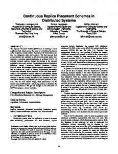
C. Simulation Results Table II shows the range of parameters used for the simulations. Typical values for practical systems are used for all parameters, except for the mean times to failure of a node, which have been chosen artificially low (10000 h, 1000 h, and 400 h for replication factors 2, 3, and 4, respectively) to run the simulations fast. The running times of simulations with practical values of the mean times to node failure, which are of the order of 10000 h or higher, are prohibitively high; this is due to the fact that PDL becomes extremely low (of the order of 10−6 ) thereby making the number of first-node-failure events that need to be simulated (along with the other complex set of events that restore all lost replicas following each firstnode-failure event) extremely high (of the order of 106 ) for each run of the simulation for a given set of parameters. Although this approach scales down the MTTDL by making failure events more frequent, its use is justified (as in [9]) because it preserves the ratios of MTTDLs of the various schemes. Replication Factor 2: Fig. 1 shows the comparison of theoretically predicted and simulation-based MTTDL values for a system with replication factor 2 and mean time to failure of a node, 1/λ, equal to 10000 h as the number of nodes n in the system is varied. It is observed that the theoretically predicted values, although approximate, are a good match to the simulation-based values as they typically lie within the 95% confidence intervals. From (17) and (20), for r = 2, MTTDLclus. MTTDLdeclus.

≈ ≈

b/(ncλ2 ), b/(2ncλ2 ).

5

10

10

4

3

clustered (theoretical) clustered (simulated) declustered (theoretical) declustered (theoretical)

2

10 0 10

1

10 Number of nodes

10

2

Comparison of theoretically predicted and simulated values of MTTDL for a replication factor of two with mean time to failure of a node equal to 10000 h. For the simulated results, 95% bootstrap confidence intervals are shown. Fig. 1.

r=2 1/λ = 10000h −2

P

DL

10

P

clustered (theoretical)

P

clustered (simulated)

P

declustered (theoretical)

P

declustered (simulated)

DL

10

−3

DL DL DL

0

1

10

(21) (22)

10 Number of nodes

10

2

Comparison of theoretically predicted and simulated values of PDL for a replication factor of two with mean time to failure of a node equal to 10000 h. For the simulated results, 95% bootstrap confidence intervals are shown. Fig. 2.

Both the clustered and the declustered placement schemes have an MTTDL that is inversely proportional to the number of nodes, with the declustered placement having a slightly worse MTTDL (by a factor of two) than the clustered. This result is similar to that obtained in [2] for exponentially distributed rebuild times. Fig. 2 shows the comparison of theoretically predicted and simulation-based PDL values which also shows agreement between theory and simulation. Thus the MTTDL approximation (2) is quite good for the set of parameters considered. Replication Factor 3: Theoretical estimates of MTTDL match well with the simulation-based values as seen in Fig. 3. Note that the approximations made in the theoretical analysis, which hold for λc/b ! 1, are still valid for the case shown in Fig. 3, where λc/b ≈ 0.035. Similar agreement is seen for the values of PDL in Fig. 4. From (17) and (20), for replication factor

r = 3, we get MTTDLclus.

≈

b2 /(nc2 λ3 ),

(23)

declus.

≈

(n − 1)b2 /(4nc2 λ3 ).

(24)

MTTDL

As seen from the above equations and also from Fig. 3, the MTTDL of clustered placement is inversely proportional to the number of nodes, whereas the MTTDL of declustered placement is essentially independent of the number of nodes. The reason is that, for declustered placement, if a second node failure occurs during the rebuild of the first node, the amount of data that become critically exposed (that is, having only one copy left) is inversely proportional to n; whereas for clustered placement, it is independent of n (see (7) and (8)).

333!444

10

5

10

6

r=4 1/λ = 400h

r=3 1/λ = 1000h

10

10

MTTDL (in days)

MTTDL (in days)

10 4

3

clustered (theoretical) clustered (simulated) declustered (theoretical) declustered (simulated)

10

4

clustered (theoretical) clustered (simulated) declustered (theoretical) declustered (simulated)

3

2

2

10 0 10

1

10 Number of nodes

10

10 0 10

2

1

10 Number of nodes

−2

10

−3

r=4 1/λ = 400h 10

−4

P

DL

DL

−3

P

10

−4

P

clustered (theoretical)

P

clustered (simulated)

P

declustered (theoretical)

DL DL DL

10

−5

10

0

1

10 Number of nodes

clustered (simulated)

DL

PDL declustered (simulated) 10

10

2

≈

b3 /(nc3 λ4 ),

≈

(n − 1)2 (n − 2)b3 /(24nc3 λ4 ). (26)

1

10 Number of nodes

10

2

Comparison of theoretically predicted and simulated values of PDL for replication factor four with mean time to failure of a node equal to 400 h. For the simulated results, 95% bootstrap confidence intervals are shown.

Replication Factor 4: Although there is a difference between theoretical and simulation results on MTTDL and PDL as seen in Fig. 5 and Fig. 6 respectively, their behavior with respect to the number of nodes is well captured by the theoretical analysis. The MTTDL of declustered placement increases with the number of nodes which is contrary to common intuition which may suggest that larger systems are less reliable. From (17) and (20), for replication factor r = 4, declus.

0

Fig. 6.

PDL for replication factor three with mean time to failure of a node equal to 1000 h. For the simulated results, 95% bootstrap confidence intervals are shown.

MTTDLclus.

−7

10

Fig. 4. Comparison of theoretically predicted and simulated values of

MTTDL

clustered (theoretical)

P

PDL declustered (theoretical)

−5

10

P

DL

−6

PDL declustered (simulated) 10

2

Fig. 5.

r=3 1/λ = 1000h

10

10

Comparison of theoretically predicted and simulated values of MTTDL for replication factor four with mean time to failure of a node equal to 400 h. For the simulated results, 95% bootstrap confidence intervals are shown.

Comparison of theoretically predicted and simulated values of MTTDL for replication factor three with mean time to failure of a node equal to 1000 h. For the simulated results, 95% bootstrap confidence intervals are shown. Fig. 3.

10

10

5

1/(nλPDL ) by ignoring the time periods spent by the system during its rebuilds, and the second is when we approximate the probability of all paths to data loss by probability of the direct path to data loss. The first approximation is valid when assumption (1) can be justified and PDL is computed without approximation. However, the second approximation of computing the probability of direct path to data loss instead of PDL is also affected by both the validity of the assumption (1) and this effect is compounded by the number of exposure levels (which in turn is equal to the replication factor). Therefore, it is expected that PDL is underestimated (and therefore the MTTDL is overestimated) by this approximation for higher replication factors and when failure rates are high.

(25)

The difference between theory and simulation is attributed to the fact that we make two levels of approximation in the theoretical analysis: first is when we approximate MTTDL by

333!555

The reliability in terms of MTTDL was derived by considering the direct path to data loss after the first node failure. In this paper, we applied this method to analyze a system model in which node failures are independent. However, it is likely that it can be used in future work to also investigate the effect of correlated failures. The inclusion of factors like delay in the start of rebuild after a node failure and network bandwidth constraint in the model are also of interest for future work as these make the model more realistic. Other directions for further research are consideration of failure distributions that not exponential, and the effect of placement of erasure coded stripes on reliability.

D. Summary of Findings The following lists the findings of this work: • The MTTDL, as can be seen in (17) and (20) is proportional to (b/c)r−1 /λr . Typically, in the literature [4], a rebuild rate µ is defined as µ := b/c and we have the commonly observed factor µr−1 /λr in the expressions of MTTDL; this matches with our results. • For clustered placement, the MTTDL is inversely proportional to the number of nodes n. This has also been observed in literature [4]. • For a replication factor of two, the MTTDLs of clustered and declustered placements differ only by a factor of two. • For replication factors greater than two, the MTTDL behaviors of the two placement schemes with respect to n differ significantly. The MTTDL of clustered placement is inversely proportional to n for all replication factors, whereas the MTTDL of declustered placement is propor1 tional to n 2 r(r−3) where r is the replication factor. • The MTTDL of declustered placement scheme decreases inversely proportional to n for a replication factor of two, stays constant with n for a replication factor of three, and 1 increases proportional to n 2 r(r−3) for replication factors greater than three. In contrast, the MTTDL of clustered placement scheme decreases inversely proportional to n for all replication factors. • The significant difference in the MTTDLs of clustered and declustered placements arises not because of the fact that the time taken to rebuild the same amount of data is significantly different – in fact, for the same amount of data to be rebuilt, the probability of exposure level transitions is approximately the same for both placements – but because of the fact that the amount of most exposed data to be rebuilt at higher exposure levels is significantly different.

A PPENDIX A P ROBABILITY OF A LL PATHS TO DATA L OSS VS . THE P ROBABILITY OF THE D IRECT PATH TO DATA L OSS Let qj→r , j = 1, 2, · · · , r − 1, denote the probability that, once the system has entered exposure level j, it goes to exposure level r prior to going to exposure level j − 1. Note that the probability of the direct path to data loss following the first node failure is then equal to q1→r . Let the probability Pj→j+1 that the system goes from exposure level j to j +1 be equal to $j . For highly reliable systems, (11) and (14) reveal that $j ! 1. We now proceed to derive qj→r , by conditioning on the subsequent transition given that the system is at exposure level j. It follows that qj→r = $j h(j+1)→r + (1 − $j ) 0 , for j = 1, · · · , r − 1, (27) where h(j+1)→r denotes the probability that once the system has entered exposure level j + 1, it goes to exposure level r prior to going to exposure level j − 1. This probability is derived by conditioning on which of the two exposure levels j and r is subsequently entered first, that is, for j = 1, · · · , r−1, h(j+1)→r = q(j+1)→r + (1 − q(j+1)→r ) qj→r .

VIII. C ONCLUSIONS

(28)

The first term of the summation accounts for the event that exposure level r is entered first, whereas the second term accounts for the event that exposure level j is entered first. In the latter case, the probability that the exposure level r is subsequently entered prior to entering exposure level j − 1 is given by qj→r , according to its definition. Combining (27) and (28) yields, for j = 1, · · · , r − 1,

In this paper, we compared the reliability of two placement schemes, namely, clustered and declustered, in terms of the MTTDL. Rebuilds play an important role in determining the reliability of a system and these two schemes represent the two extremes of the degree of parallelism that can be exploited during rebuild. Declustered placement spreads replicas of data on each node across all other nodes and hence enables maximum parallelism during rebuild, whereas clustered placement spreads replicas of data on each node across the minimum possible number of nodes and therefore minimizes the degree of parallelism. Our results demonstrated that, the MTTDL of the clustered placement scheme is inversely proportional to the number of nodes for any replication factor. In contrast, for the declustered placement scheme with replication factors greater than two, contrary to intuition, the MTTDL does not decrease as the number of nodes increases; it remains constant for a replication factor of three, and increases for a replication factor greater than three. The theoretical estimates match well with the simulation results obtained.

qj→r = $j (q(j+1)→r + (1 − q(j+1)→r ) qj→r ).

(29)

Solving (29) for qj→r yields the recursive relation $j q(j+1)→r , for j = 1, · · · , r − 1. (30) qj→r = 1 − $j (1 − q(j+1)→r ) In particular, for $j ! 1, it follows that qj→r ≈ $j q(j+1)→r ,

for j = 1, · · · , r − 1.

(31)

Consequently, repeatedly applying (31) yields qj→r ≈

r−1 # i=j

333!666

$i ,

for j = 1, · · · , r − 1.

(32)

˜

Note that the product on the right hand side of the above equation is equal to the probability of occurrence of the direct path j → j + 1 → · · · → r from exposure level j to data loss. Thus, for j = 1, Eq. (32) leads to the result sought: PDL = q1→r ≈

r−1 #

where θ = e−λζ for some ζ, 0 ≤ ζ ≤ y (Taylor’s theorem). So, it follows that θ# ˜ 2 ˜ ˜ Pr{F < R} = λE[R] − λ E[R2 ] ≈ λE[R], 2 where the equality follows by integration yielding θ# between 0 and 1 (because 0 ≤ θ ≤ 1), and the approximation follows from the assumptions (34) and (35) on fR (·). Similarly, ˜ − x)E[R], Pr{F < R(1 − x)} ≈ λ(1

$i , for $i ! 1, i = 1, · · · , r − 1, (33)

i=1

namely, for a highly reliable system, the probability that, once the system has entered exposure level one, it goes to exposure level r prior to reaching exposure level zero, is equal to the probability of the direct path 1 → 2 → · · · → r to data loss for a highly reliable system.

as x ∈ (0, 1]. Therefore, plugging the above two equations in (36), we get Pr{α ≤ x} ≈ x,

A PPENDIX B F RACTION OF DATA R EBUILT

This means that, for highly reliable systems, α is uniformly distributed between zero and one.

Suppose that a node failure occurred at time zero, and a certain amount of data has to be rebuilt before another node ˜ Let R be the time taken to failure occurs at time F ∼ Exp(λ). complete rebuilding the data and let fR (·) be the probability density function of R such that ˜ 2 E[R2 ])/(λE[R]) ˜ (λ →0 ˜ λE[R]

as

˜ λE[R] → 0,

(34)

!

1.

(35)

R EFERENCES [1] C. Miller, A. R. Butt, and P. Butler, “On utilization of contributory storage in desktop grids,” in Proc. IEEE International Parallel and Distributed Processing Symposium (IPDPS’08), April 2008, pp. 1–12. [2] V. Venkatesan, I. Iliadis, X.-Y. Hu, R. Haas, and C. Fragouli, “Effect of replica placement on the reliability of large-scale data storage systems,” in Proc. 18th Annual IEEE/ACM International Symposium on Modeling, Analysis, and Simulation of Computer and Telecommunication Systems (MASCOTS’10), 2010, pp. 79–88. [3] K. M. Greenan, E. L. Miller, and J. Wylie, “Reliability of flat XORbased erasure codes on heterogeneous devices,” in Proc. 38th Annual IEEE/IFIP International Conference on Dependable Systems and Networks (DSN’08), June 2008, pp. 147–156. [4] S. Ramabhadran and J. Pasquale, “Analysis of long-running replicated systems,” in Proc. 25th IEEE International Conference on Computer Communications (INFOCOM’06), 2006, pp. 1–9. [5] M. Leslie, J. Davies, and T. Huffman, “A comparison of replication strategies for reliable decentralised storage,” Journal of Networks, vol. 1, no. 6, pp. 36–44, December 2006. [6] A. Thomasian and M. Blaum, “Mirrored disk organization reliability analysis,” IEEE Transactions on Computers, vol. 55, pp. 1640–1644, December 2006. [7] Q. Xin, E. L. Miller, T. Schwarz, D. D. E. Long, S. A. Brandt, and W. Litwin, “Reliability mechanisms for very large storage systems,” in Proc. 20th IEEE / 11th NASA Goddard Conference on Mass Storage Systems and Technologies (MSS’03), 2003, pp. 146–156. [8] Q. Xin, E. L. Miller, and T. J. E. Schwarz, “Evaluation of distributed recovery in large-scale storage systems,” in Proc. 13th IEEE International Symposium on High Performance Distributed Computing (HPDC’04), 2004, pp. 172–181. [9] Q. Lian, W. Chen, and Z. Zhang, “On the impact of replica placement to the reliability of distributed brick storage systems,” in Proc. 25th IEEE International Conference on Distributed Computing Systems (ICDCS’05), 2005, pp. 187–196. [10] W. Jiang, C. Hu, Y. Zhou, and A. Kanevsky, “Are disks the dominant contributor for storage failures?: A comprehensive study of storage subsystem failure characteristics,” ACM Transactions on Storage, vol. 4, no. 3, pp. 1–25, November 2008. [11] S. Nath, H. Yu, P. B. Gibbons, and S. Seshan, “Subtleties in tolerating correlated failures in wide-area storage systems,” in Proc. 3rd conference on Networked Systems Design & Implementation (NSDI’06), 2006, pp. 225–238. [12] D. Ford, F. Labelle, F. I. Popovici, M. Stokely, V.-A. Truong, L. Barroso, C. Grimes, and S. Quinlan, “Availability in globally distributed storage systems,” in Proc. 9th USENIX Symposium on Operating Systems Design and Implementation (OSDI’10), 2010, pp. 61–74. [13] K. M. Greenan, J. S. Plank, and J. J. Wylie, “Mean time to meaningless: MTTDL, Markov models, and storage system reliability,” in Proc. of the USENIX Workshop on Hot Topics in Storage and File Systems (HotStorage), 2010, pp. 1–5. [14] A. Thomasian and M. Blaum, “Higher reliability redundant disk arrays: Organization, operation, and coding,” ACM Trans. Storage, vol. 5, no. 3, pp. 1–59, 2009.

Note that fixed and exponentially distributed rebuild times satisfy (34). Also it can be shown that (35) is true for both clustered and declustered placements in a highly reliable system as follows. For clustered placement at exposure level ˜ = (r −e)λ. Also, from (7) and (9), it follows that E[R] ≤ e, λ ˜ c/b. So, by assumption (1), λE[R] ≤ (r − e)λc/b ! 1. For ˜ = (n−e)λ. From declustered placement at exposure level e, λ (8) and (12), it follows that E[R] ≤ c/((n − e)b/2). So, again ˜ by assumption (1), λE[R] ≤ 2λc/b ! 1. We are interested in the fraction of data that is not rebuilt when a node failure happens, given that this failure happens before rebuild completes, that is, given that F < R. Assuming that the amount of data rebuilt during a time period is proportional to that time period, the fraction of data not rebuilt, α, is α = (R − F )/R,

for

F < R.

The distribution function of α for x ∈ (0, 1] is Pr{α ≤ x} = = = =

x ∈ (0, 1].

Pr { (R − F )/R ≤ x| F < R} Pr{R(1 − x) ≤ F < R} Pr{F < R} Pr{F < R} − Pr{F < R(1 − x)} Pr{F < R} Pr{F < R(1 − x)} 1− . (36) Pr{F < R}

Now, consider Pr{F < R}: & ∞ ˜ Pr{F < R} = (1 − e−λy )fR (y)dy % &0 ∞ $ ˜ 2 y 2 fR (y)dy ˜ − θλ λy = 2 0

333!777