Reliability of marker based tracking in comparison to

Reliability of marker based tracking in comparison to silhouette based tracking: Inter-Tester Reliability and Intra-Subject Reliability

Master‘s thesis

by Patricia Schütz

German Sports University Cologne Cologne 2018

Reliability of marker based tracking in comparison to silhouette based tracking: Inter-Tester Reliability and Intra-Subject Reliability

Master‘s thesis

by Patricia Schütz

German Sports University Cologne Cologne 2018

Supervisor: Dr., Steffen Willwacher, Institut für Biomechanik und Orthopädie

Table of content 1

Introduction.............................................................................................. 1 1.1

The Gait Cycle .................................................................................. 1

1.2

Reliability as quality requirement for analyses .................................. 3

1.3

Marker-based tracking ...................................................................... 3

1.3.1

Advantages and disadvantages ................................................. 4

1.3.2

Studies about reliability .............................................................. 5

1.4

1.4.1

Advantages and disadvantages ................................................. 8

1.4.2

Studies about accuracy .............................................................. 8

1.5 2

Motivation and aim of the thesis ..................................................... 10

Theoretical background ......................................................................... 11 2.1

3

Markerless tracking ........................................................................... 7

Anatomical and biomechanical foundations .................................... 11

2.1.1

Body planes and axes .............................................................. 11

2.1.2

The human joint and its possible movements .......................... 12

2.2

Technical equipment, system setup and calibration ....................... 14

2.3

Methods of motion tacking .............................................................. 16

2.3.1

Marker-based tracking in Simi Motion ...................................... 17

2.3.2

Silhouette-based markerless tracking in Simi Shape ............... 19

2.3.3

Marker-based tracking in Simi Shape....................................... 21

Materials and methods .......................................................................... 22 3.1

Hypotheses for the evaluation ........................................................ 22

3.2

Data collection and processing ....................................................... 23

3.2.1

Set-up, subject and procedure ................................................. 23

3.2.2

Differences of calculation templates ......................................... 24

3.2.3

Marker-based data ................................................................... 25

3.2.4

Silhouette-based data .............................................................. 26

3.3

Parameters of interest..................................................................... 26

3.4 4

Results .................................................................................................. 33 4.1

Differences of calculation templates ............................................... 33

4.2

Accuracy ......................................................................................... 35

4.3

Inter-Tester Reliability ..................................................................... 38

4.3.1

Temporal-spatial parameters ................................................... 38

4.3.2

Kinematic - joint angles ............................................................ 39

4.3.3

Kinematic - joint centers ........................................................... 40

4.4

Intra-Subject Reliability ................................................................... 42

4.4.1

Temporal-spatial parameters ................................................... 42

4.4.2

Kinematic - joint angles ............................................................ 43

4.4.3

Kinematic - joint centers ........................................................... 44

4.5 5

Statistical analysis .......................................................................... 28

Range of motion ............................................................................. 47

Discussion ............................................................................................. 48 5.1

Differences in calculation templates ............................................... 48

5.2

General: silhouette-based tracking vs. marker-based tracking ....... 49

5.3

Inter-Tester Reliability ..................................................................... 50

5.4

Intra-Subject Reliability ................................................................... 52

5.5

Reliability ........................................................................................ 53

5.6

Fields of application and possible motion analysis systems ........... 55

6

Conclusion and outlook to further possibilities of investigation .............. 58

7

References ............................................................................................... I

Appendix A – Marker positions ..................................................................... VI Appendix B – overall coefficient of variance ................................................ VII Appendix C - LFM left step ......................................................................... VIII Appendix D – figures local joint angles ......................................................... IX Appendix E – figures joint centres............................................................... XXI

List of figures Figure 1: Distribution of the human gait cycle [3] ............................................ 1 Figure 2: (a) Multiple perspectives of high-speed-camera recordings (b) Automatic 3D-silhouette extraction................................................... 7 Figure 3: Body planes and axes [22]............................................................. 11 Figure 4: Different types of joints [25] ........................................................... 13 Figure 5: Joint movements [27] ..................................................................... 14 Figure 6: Camera with ring lights [28] ........................................................... 15 Figure 7: Calibration tools: T-wand and L-frame [28] .................................... 15 Figure 8: Local segment coordinate systems (red: x-axes, green: y-axes, blue: z-axes) [28]............................................................................ 17 Figure 9: Jump in the curve of the inner ankle bone along the frontal axis ... 18 Figure 10: Missing marker visual in the 3D stick view in comparison: (a) 3D stick view without errors

(b) 3D stick view with missing

connecting line, because of a missing hip marker .......................... 19 Figure 11: 3D automatic model pose estimation: (a) Segmentation in each camera view (b) Overlay of the model ................................... 20 Figure 12: Camera set-up a) Gait laboratory University Regensburg and laboratory of Simi Reality Motion Systems GmbH b) Gait laboratories Schönklinik Bad Aibling and Hospital Rummelsberg .. 24 Figure 13: Marker model lower extremities ................................................... 25 Figure 14: Joint center movement of the right ankle along the longitudinal axis – while one color stands for one trial, dashed lines are tracked in Simi Shape and drawn lines are tracked in Simi Motion ............................................................................................ 34 Figure 15: Joint center movement of the right hip along the longitudinal axis – while one color stands for one trial, dashed lines are tracked in Simi Shape and drawn lines are tracked in Simi Motion ............................................................................................ 35 Figure 16: Two exemplary datasets were compared in order to graphically illustrate the different LFM results - all trials (colored) and reference data (gray) – (a) Well fitted knee right flexion/ extension (b) Not fitting ankle right adduction/ abduction ............... 37

Figure 17: Mean curves of each lab and tracking variant (silhouettebased S drawn lines and marker-based M dashed lines) of the hip adduction/ abduction – lab 1 = Rummelsberg; lab 2 = Bad Aibling; lab 3 = Bad Abbach (M) or Simi (S); gray = reference data ................................................................................................ 40 Figure 18: Mean curves of each lab and tracking variant (silhouettebased S drawn lines and marker-based M dashed lines) of the hip joint center movement along the frontal axis – lab 1 = Rummelsberg; lab 2 = Bad Aibling; lab 3 = Bad Abbach (M) or Simi (S) .......................................................................................... 42 Figure 19: All marker-based trials in the gait laboratory in Bad Aibling a) Excellent correlation: right ankle along the longitudinal axis b) No correlation: right ankle along the frontal axis ............................ 46 Figure 20: joint center movement of the left knee along the frontal axis showing a low correlation ............................................................... 49 Figure 21: exemplary curve showing a bad LFM result although it visually looks accurate ................................................................................ 50 Figure 22: Shadow in the segmentation due to the ring lights ...................... 55

List of tables Table 1: Overview of marker based reliability studies in gait analysis for the right side (Tsushima et al. average between both sides) – the results show CMC in percent ± std. for joint angles. Correlations that are ≥ 0.9 are highlighted in green, those ≥ 0.7 in yellow and correlations of less than 0.7 are highlighted in red. .... 5 Table 2: Overview of marker based reliability studies in gait – the results show CV in percent ± std. ................................................................ 6 Table 3: Overview of studies comparing marker-based and silhouettebased analyses for joint angles ........................................................ 9 Table 4: Used cameras and camera settings.............................................. 23 Table 5: Parameters analyzed .................................................................... 27 Table 6: Pearson's correlation for the comparison of the calculation templates in Simi Motion and Simi Shape – worse correlations (ρ < 0.72) are highlighted in red ..................................................... 33 Table 7: LFM right leg. Correlations that are ≥ 0.95 are highlighted in dark green, those that are ≥ 0.85 in bright green, those ≥ 0.75 in yellow, those ≥ 0.60 in orange and correlations of less than 0.60 are highlighted in red. ..................................................................... 36 Table 8: Inter-Tester Coefficient of variance (CV) [%] of temporal-spatial parameters for silhouette-based and marker-based tracking ......... 38 Table 9: Inter-Tester Coefficient of multiple correlation (CMC) of joint angles

for

silhouette-based

and

marker-based

tracking.

Correlations that are ≥ 0.95 are highlighted in dark green, those that are ≥ 0.85 in bright green, those ≥ 0.75 in yellow, those ≥ 0.60 in orange and correlations of less than 0.60 are highlighted in red. ............................................................................................. 39 Table 10: Inter-Tester Coefficient of multiple correlation (CMC) of joint centers for silhouette-based and marker-based tracking. Correlations that are ≥ 0.95 are highlighted in dark green, those that are ≥ 0.85 in bright green, those ≥ 0.75 in yellow, those ≥ 0.60 in orange and correlations of less than 0.60 are highlighted in red. ............................................................................................. 41

Table 11: Intra-Subject Coefficient of variance (CV) [%] of temporalspatial parameters for silhouette-based and marker-based tracking .......................................................................................... 43 Table 12: Intra-Subject Coefficient of multiple correlation (CMC) of joint angles

for

silhouette-based

and

marker-based

tracking.

Correlations that are ≥ 0.95 are highlighted in dark green, those that are ≥ 0.85 in bright green, those ≥ 0.75 in yellow, those ≥ 0.60 in orange and correlations of less than 0.60 are highlighted in red. ............................................................................................. 44 Table 13: Intra-Subject Coefficient of multiple correlation (CMC) of joint centers for silhouette-based and marker-based tracking. Correlations that are ≥ 0.95 are highlighted in dark green, those that are ≥ 0.85 in bright green, those ≥ 0.75 in yellow, those ≥ 0.60 in orange and correlations of less than 0.60 are highlighted in red. ............................................................................................. 45 Table 14: Mean, std. and corresponding reference values of RoM of joint angles for silhouette-based tracking ....................................... 47 Table 15: Mean, std. and corresponding reference values of RoM of joint angles for marker-based tracking ........................................... 47 Table 16: Reference data of temporal-spatial parameters .......................... 51 Table 17: Mean and std. of CV for silhouette-based and marker-based tracking .......................................................................................... 51 Table 18: Comparison between Inter-Tester and Intra-Subject reliability for right joint center movements. Correlations that are ≥ 0.95 are highlighted in dark green, those that are ≥ 0.85 in bright green, those ≥ 0.75 in yellow, those ≥ 0.60 in orange and correlations of less than 0.60 are highlighted in red. ...................... 53 Table 19: gait parameters for different fields of application [41]: green highlighted can be recommended for both methods, yellow highlighted can be limited highlighted and red highlighted cannot be recommended for any method. ...................................... 57 Table 20: Overall Coefficient of variance (CV) [%] of temporal-spatial parameters for silhouette-based tracking ...................................... VII

Table 21: Overall Coefficient of variance (CV) [%] of temporal-spatial parameters for marker-based tracking .......................................... VII Table 22: LFM left step. Correlations that are ≥ 0.95 are highlighted in dark green, those that are ≥ 0.85 in bright green, those ≥ 0.75 in yellow, those ≥ 0.60 in orange and correlations of less than 0.60 are highlighted in red. ................................................................... VIII

1 Introduction Gait analysis is an important tool to understand the human walking. It is used in several fields of application like orthopedics, physiotherapy or chirurgic as diagnostic and treatment planning aid for functional gait disorders. Especially in the sports and clinical application a high accuracy and robustness is required. Additionally, a minimal patient preparation time and inter-observer variability should be guaranteed. [1] Therefor marker-based video analysis is still the gold standard as it has a very high accuracy. In the last years more and more studies were done evaluating silhouette-based tracking. This study compares the reliability of marker-based tracking in comparison to silhouettebased tracking.

1.1 The Gait Cycle The gait can be divided into a single sequence which is repeated continuously. This sequence is called gait cycle. It starts with the Initial Contact (IC) of the floor and ends with the ipsilateral IC. First one limb is used to support while the other limb advances itself forward to a new support site. Afterwards the two limbs switch their roles. [2]

Figure 1: Distribution of the human gait cycle [3]

1

The gait cycle is divided into two phases: stance and swing (Figure 1). For an average walking velocity, the stance phase lasts 60 percent, while the swing phase lasts 40 percent of the gait cycle. The stance phase can be subclassified into three phases. The Initial Double Limb Stance starting with the ipsilateral IC, which is also called Double Limb Support. The body weight is shared equally between both feet. Lifting the opposite foot for the swing is the starting time point for the Single Limb Stance. The duration of this phase is an indicator for the stability of the limb. The last phase is the Terminal Double Limb Stance, which starts with the contralateral IC and ends with the ipsilateral toe off. Another possibility of splitting a gait cycle is dividing it by step and stride. One stride is equal to one gait cycle and therefore the interval between two sequential IC of the same limb. One step refers to the timing between both limbs. As one step is the interval between the IC by one foot, two steps are one stride. [2] The Rancho Los Amigos Gait Analysis Committee [4] introduced a generic terminology for dividing the phases of a gait due to its functionalities. In total eight functional gait phases exist each having a functional obejective. As the functional needs change in one stride, joint movements can be appropriate in one phase but can signify a dysfunction in another gait phase. Like this it is important to separate the gait cycle into eight phases. In each timing and joint angles are than significant. The phases Initial Contact (IC) and Loading Response have the task of weight acceptance. The main tasks are: shock absorption, stability of the initial limb and the preservation of progression. Mid Stance and Terminal Stance are involved into the Single Limb Support. The last four gait phases Pre-Swing, Initial Swing, Mid Swing and Terminal Swing have the task to advance the swing limb. [2]

2

1.2 Reliability as quality requirement for analyses All scientific tests, as gait analysis, have to fulfill three aspects. First it must be checked whether the test measures what it claims to measure. This refers to the stability or consistency of the measurement. This aspect is called validity. In statistical terms this is the unbiasedness. A further important point is the objectivity. The measurement outcome and conclusion has to be independent from the operator. Last aspect, which has to be fulfilled, is the reliability, which refers to the suitability or meaningfulness of the measurement. When a trial is repeated under identical conditions the outcome of the measurement has to be the same. A low reliability follows in a high statistical variance. [5, 6] All measurements are subject to fluctuations. These errors can affect the measurement’s reliability and validity. Like this each observed score can be divided into the two parts: true score and error. A test is reliable if the error is minimal. The reliability coefficient is the proportion of true variability to the observed variability. A reliability coefficient of 90 percent, for example, means that 90 percent of the variability represents the true individual differences and 10 percent of the variability is due to random error. Reliability is a correlation computed between two events. The Test-retest reliability or stability tests the same subject with exactly the same test at two different points in time. The correlation coefficient between both data sets describes the degree of reliability. [5]

1.3 Marker-based tracking The standard technology of motion capture nowadays is marker-based tracking. It uses retroreflective markers, which are recognized and assigned to a specific anatomical landmark by a software.

3

1.3.1 Advantages and disadvantages Marker-based tracking has a very high accuracy. Bader [7] conducted a mean failure smaller than 0.1 mm for the software Simi Motion. Still a high accuracy in marker detection does not gather high measurement accuracy as joint center movements or joint angles are calculated out of a model optimization. Another advantage is that fast and explosive movements can be analyzed due to the possibility of high capture frames. Attaching at least three markers to each body segment, allows the registration of movements of all segments in all planes. Besides these positive properties some problems and disadvantages still occur with marker-based tracking. Leardini et al. [8] stated that soft tissue artefacts are the most critical source of error. The offset between a marker and its anatomical reference point can be measured using the invasive methods intra-cortical pins or X-rays. Lafortune et al. [9] measured with the intra-cortical pins a marker displacement in unloaded knee flexion-extension up to 23 mm. Reinschmidt el al. [10] investigated marker displacement during walking or running. The authors measured a knee joint angle error relative to the range of motion of 21 % for flexion/ extension, 63 % for internal/ external rotation and 70 % for abduction/ adduction. Soft tissue artifacts were mentioned as main source of the high knee rotation errors. Another limitation of marker-based analysis is the difficult placement of markers. Three main factors cause this error: The relevant anatomical landmarks are large surfaces and/ or not prominent. The soft tissue layers covering the subcutaneous bony landmarks differ in thickness and composition. And last several palpation procedures exist to identify the anatomical landmarks. [11] The next possible error source is the subjects’ change of their natural way of movement due to the markers. First, they can change their movement pattern due to the risk of losing markers. Second, artificial stimuli can produce unwanted artifacts masking the natural movement pattern. Especially in elite athletes these artificial stimuli to the neurosensory system can lead to subtle changes

in

the

movement

patterns.

Their

coordination

skills

and

sensorimotor awareness are sensible for these subtle influences due to external factors like markers or new laboratory environment. [12]

4

The last disadvantage is the high patient preparation time. Becker [13] measured the time, which is needed for marker placement with an average of 31 markers. Therefor a time of 18 minutes was needed in average. Additional time should be calculated for the case that markers get loosen during the measurement and to give the patient time to familiarize with the marker positions. Especially in the clinical daily routine, this is a substantial amount of time.

1.3.2 Studies about reliability Several studies exist evaluating the reliability of marker based systems. Their results for kinematic joint angle data are summarized in Table 1 (Coefficient of multiple correlation (CMC)) and Table 2 (Coefficient of variation (CV)). Table 1: Overview of marker based reliability studies in gait analysis for the right side (Tsushima et al. average between both sides) – the results show CMC in percent ± std. for joint angles. Correlations that are ≥ 0.9 are highlighted in green, those ≥ 0.7 in yellow and correlations of less than 0.7 are highlighted in red.

Results

Study

System Compar/ ison cameras

Sagittal plane

Hip

Knee Ankle Pelvis Hip

0.959 0.992 Between± ± Expert day 0.028 0.004 Growney VisionTM et al. [14] / 0.996 0.997 Within4 ± ± day 0.002 0.001

Tsushima et al. [15]

Piotter et al. [16]

Kadaba et al. [17]

Vicon / 4

BTS elite motion system / 4

Vicon / 5

Frontal plane

Transversal plane

Knee Ankle Pelvis Hip

Knee Ankle Pelvis

0.964 ± 0.022

-

0.896 0.432 0.477 ± ± ± 0.041 0.136 0.074

-

0.576 0.407 0.422 ± ± ± 0.325 0.116 0.179

-

0.982 ± 0.008

-

0.978 0.911 0.766 ± ± ± 0.006 0.084 0.091

-

0.953 0.865 0.835 ± ± ± 0.021 0.052 0.063

-

IntraSubject

0.997 0.994 0.981 0.525 0.980 0.925 ± ± ± ± ± ± 0.001 0.002 0.005 0.095 0.006 0.019

-

0.984 0.927 0.857 0.884 0.920 ± ± ± ± ± 0.007 0.030 0.099 0.062 0.087

InterTester

0.984 0.992 0.974 0.448 0.963 0.782 ± ± ± ± ± ± 0.014 0.003 0.007 0.203 0.024 0.179

-

0.971 0.799 0.764 0.767 0.888 ± ± ± ± ± 0.172 0.172 0.150 0.122 0.100

Testretest

0.993 0.992 0.975 0.376 0.966 0.793 ± ± ± ± ± ± 0.005 0.003 0.010 0.142 0.019 0.163

-

0.975 0.826 0.812 0.818 ± ± ± ± 0.012 0.120 0.121 0.106

InterTester

0.986 0.988 0.904 0.442 0.930 0.571 0.804 0.893 0.462 0.507 0.858 0.814 ± ± ± ± ± ± ± ± ± ± ± ± 0.010 0.008 0.051 0.236 0.070 0.218 0.153 0.121 0.188 0.229 0.089 0.093

IntraTester

1.00 0.946 0.969 0.774 0.949 0.725 0.923 0.935 0.687 0.779 0.903 0.814 ± ± ± ± ± ± ± ± ± ± ± ± 0.003 0.084 0.018 0.066 0.024 0.208 0.042 0.038 0.159 0.080 0.009 0.093

Betweenday

0.978 0.985 0.985 0.240 0.882 0.783 ± ± ± ± ± ± 0.019 0.009 0.009 0.197 0.101 0.159

-

0.883 0.483 0.534 0.612 0.768 ± ± ± ± ± 0.104 0.236 0.221 0.200 0.154

Withinday

0.995 0.994 0.978 0.643 0.957 0.962 ± ± ± ± ± ± 0.005 0.003 0.010 0.180 0.088 0.029

-

0.956 0.893 0.918 0.885 0.878 ± ± ± ± ± 0.045 0.072 0.053 0.053 0.069

5

Table 2: Overview of marker based reliability studies in gait – the results show CV in percent ± std. Study

Growney et al. [14] Tsushima et al. [15] Kadaba et al. [17]

comparison Between-day Within-day Within-session Between-session Between-day Within-day

Statistical value CV CV CV

Results Cadence (

𝑠𝑡𝑒𝑝𝑠

𝑚

Walking speed ( )

Stride length (m)

2.46 ± 1.06

3.86 ± 0.87

2.45 ± 0.76

2.29 ± 0.86

2.69 ± 0.87

2.83 ± 0.74

1.76 ± 0.71

2.42 ± 1.04

3.62 ± 4.39

2.19 ± 0.89

3.76 ± 1.44

4.25 ± 4.25

3.4 ± 1.8

6.1 ± 7.1

3.0 ± 1.3

1.9 ± 0.8

2.9 ± 3.3

1.7 ± 0.6

𝑚𝑖𝑛

)

𝑠

Growney et al. [14] analyzed the effect of wrong marker placement by the displacement on joint angles. He gathered data while a gait analysis. First the CMC was examined for the within-day and between-day reproducibility of lower extremities joint angles. In his study, all sagittal plane movements showed good between-day and within-day results. Out-of-sagittal plane movements, especially for the knee and ankle joint, had worse correlations for the between-day reproducibility. He explained the worse between-day repeatability by the differences in marker reapplication and the skin movement relative to the underlying bones. As a result, the segment coordinate system axes are differing. The bad results for out-of-sagittal plane movements are explained by the rotations represented as Euler Angles. A rotation around a slightly incorrect x-axis results in a small error in flexion/ extension angles.

The y- and z-axes are obtained by rotating around

previously incorrect rotated axes. Thereby the errors accumulate for each rotation leading to larger errors in out-of-sagittal plane movements. Additionally, these movements have much smaller ranges of motion compared to flexion/ extension movements in the sagittal plane. The signalto-noise ratio is like this much smaller leading to wrong data. Second the CV was determined cadence, walking speed and stride length. The high reproducibility of theses time-distance parameters demonstrate that the subjects of this study walked consistently. Tsushima et al. [15] highlighted factors that contribute to variability in gait analysis: 

“Limitations in accuracy of the measurement hardware and software



Variability of walking across all trials



Reproducibility of the marker replacement across sessions (testretest) and across tester (inter-tester)



Artifacts originating from skin-marker movement” [15] 6

In his study he assessed the Intra-Subject, Inter-Tester and Test-Retest reliability for lower extremities in gait. For the Intra-Subject reliability, he did not replace the markers. The CMC was calculated for pelvic, hip, knee and ankle joint angles showing same results as Growney et al. The poor CMC value for the pelvic tilt was explained by the formula of the CMC. The CMC is decreasing, when the range of motion is smaller. The CV was very low for all three temporal-spatial parameters. Piotter et al. [16] only looked at the CMC values for Inter-Tester and Intra-Tester reliability. Between-day and withinday reliability was analyzed by Kadaba et al. [17] comparing CMC and CV. Both studies had the same results as Growney et al. and Tsushima et al.. All studies showed good reliability in sagittal plane movements of hip, knee or ankle (r ≥ 0.90) and hip abduction/adduction (r ≥ 0.88). Pelvic movements were high reliable in frontal (r ≥ 0.88) and transversal plane (r ≥ 0.77). At least in some studies worse correlations were found for all other out-ofsagittal plane movements.

1.4 Markerless tracking Several approaches of markerless analysis exist. The most established one is based on the principle of visual hull (VH). This method is also used in the software Simi Shape. It identifies and reconstructs 3D objects, especially with non-convex surfaces, out of 2D images. The VH is defined as “the locally convex (over) approximation of the volume occupied by an object” [1].

(a)

(b)

Figure 2: (a) Multiple perspectives of high-speed-camera recordings (b) Automatic 3D-silhouette extraction

7

Figure 2 shows on the left side the perspectives of several cameras of one recording. The right side shows the automatic extraction of the 2D silhouettes and the back projection of theses silhouettes from each of the camera planes back to a 3D object in space. Due to the use of a calibrated camera system, the intersection of the several 2D silhouettes can be located in the 3D space. Out of this the 3D VH of the recorded subject can be generated as point cloud or connected grid. [1] For the tracking process a mathematical full body model, consisting of connected rigid bodies, is needed. Each connection represents a joint. Therefor the translational and rotational degrees of freedom are adapted to human joints. Afterwards the model has to be scaled and fitted into the 3D silhouette. [18]

1.4.1 Advantages and disadvantages Markerless tracking offers many advantages compared to marker-based tracking. The main advantage is that no markers are needed for the tracking process leading to a high time saving. Marker-based or rater-based tracking are both based on the subjectivity of the user. A big issue in marker-based analysis is the marker attachment, which is depended on the operators’ knowledge. Rater-based analysis also needs the knowledge about anatomical landmarks. For silhouette tracking neither the position of landmarks nor the marker attachment is necessary leading to a more objective data acquisition. Another advantage due to no marker usage is the missing of skin artefacts. Last positive impact is the free and undisturbed movement of the patient. [1] A disadvantage is that silhouette-based tracking cannot detect rotations, where the silhouette only barley changes.

1.4.2 Studies about accuracy However, to become a standard technology in movement analysis, silhouette-based tracking has to be accurate, valid and reliable. In clinical and sports applications, the tracking has to be much more accurate than in the original field of application: movie and computer game industry. In sports and clinical analyses markerless tracking is still new. Anyway the accuracy has already been tested in different laboratory studies (Table 3).

8

Table 3: Overview of studies comparing marker-based and silhouette-based analyses for joint angles

Results Marker Marker-less based system system

Study

Move- Statistical ment value

Sagittal plane

Hip

RMSD [°] Oberländer BioVicon et al. [19] Stage

Own Ceseracciu appet al. [20] roach (VH)

Gait

BTS SMARTD

Gait

Own Münderappmann et al. Qualisis roach [12] (VH)

Gait

Virtual environment, Poser software

Gait

Own Corazza et appal. [1] roach (VH) Otte et al. [21]

Kinect Vicon V2

Becker [13]

Simi Simi Shape Motion

Knee Ankle

1.9

Spearman ’s 1.00 correlation SD of root mean square 8.5 deviation [°] Average deviation of the deviation of joint angles [°]

Gait + several other Movements in all joints and planes

Frontal plane

Hip

Transversal plane

Knee Ankle

Hip

Knee ankle

3.4

2.5

-

-

-

-

-

-

0.93

0.89

-

-

-

-

-

-

2.5

1.8

2.3

-

3.6

9.3

-

7.0

2.3

-

-

1.6

-

-

-

-

RMS error [°]

3.6

4.2

9.0

2.0

3.1

5.9

-

-

-

Pearson’s correlation

0.99 ± 0.05

0.87 ± 0.28

0.81 ± 0.33

0.81 ± 0.25

0.80 ± 0.21

0.64 ± 0.32

0.64 ± 0.34

0.19 ± 0.41

0.22 ± 0.38

Spearman ’s 0.86 correlation

1.00

0.98

0.97

-

0.39

0.93

-

0.58

Oberländer and Brüggemann [19] compared markerless data of hip, knee and ankle sagittal plane joint angles to marker-based data in walking. The high

correlation

(r ≥ 0.89)

and

the

low

root-mean-square

deviation

(RMSD ≤ 3.4 °) show a good alignment between both systems for analyzing lower limb joint angles in sagittal plane. Similar results were found by Ceseracciu et al. [20]

for sagittal plane movements as well as for hip

adduction/ abduction (SD RMSD ≤ 2.5 °). The worst results were found for hip internal/ external rotation with an angle deviation up to 9 °. As conclusion he stated that sagittal plane movements are comparable, while transversal plane movements are not sufficiently precise enough for applications in the clinical field. Mündermann et al. [12] and Corazza et al. [1] showed also same results. Otte et al. [21] mentioned the inherent differences between both 3D skeletons as marker-based uses surface markers and markerless 9

approaches use landmarks within the body shape. This may affect 3D Euclidean distances, but does not affect correlation analyses. Her results show worst results for foot movements explained by the high signal-to-noiseratio. The results of Becker [13] also show that small range of motion movements are the lowest comparable once. An exact comparison between all studies is not possible as they used different statistical methods and sometimes did not state the exact calculations. However, most studies show a high accuracy for hip, knee and ankle sagittal plane movements and hip and knee frontal plane movements. Low accuracy only occured for hip flexion/ extension in the study of Ceseracciu [20] and ankle dorsi-/ plantarflexion in the study from Corazza [1]. Movements with a small range of motion as ankle adduction/ abduction and hip, knee and ankle transversal plane movements show worse results. Regarding these results about the markerless tracking accuracy, a high accuracy for movements with a big RoM can be expected. Studies about reliability of markerless analysis could not be found.

1.5 Motivation and aim of the thesis As stated above there are only reliability studies for marker-based tracking. Some studies exist comparing the accuracy of marker-based to silhouettebased tracking. Nevertheless, no research projects evaluating the reliability of silhouette-based tracking or even comparing the reliability of both techniques were found. As validity, objectivity and reliability are the main aspects of an experimental measurement, the objectivity and reliability are considered in this thesis. For testing the objectivity, the Inter-Tester Reliability is analyzed. Therefore, the gait analyses of three observers are compared. The reliability of one observer is tested with the Intra-Subject Reliability. Here one subject walked ten times, after each trial the markers were replaced by the same tester. To reach the aim of this thesis, the following chapter gives a short overview of the anatomical background. Then, an overview of the used software is given. After that, the measuring methods are described, followed by the results, which are presented and discussed afterwards.

10

2 Theoretical background A short anatomical overview followed by a general description of the workflow for the used software Simi Motion and Simi Shape is given in this chapter.

2.1 Anatomical and biomechanical foundations 2.1.1 Body planes and axes

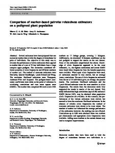
Figure 3: Body planes and axes [22]

Three different body axes divide the body to describe certain structures or directions in the anatomy. All three axes intersect in the center of mass (COM). Following those three main axes are described [23]: 

Transverse axis:

X-axis of the body, going through the COM from the left side to the right



Longitudinal axis: Y-axis of the body, going from cranial to caudal



Sagittal axis:

Z-axis of the body, going through the body from dorsal to ventral

11

Body planes are defined according to the axes [23]: 

Frontal plane:

Defined by the longitudinal and transverse axis; divides the body into a front and a back part



Sagittal plane:

Defined by the sagittal and longitudinal axis; divides the body into symmetrical right and left halfs



Transverse plane: Defined by the transverse and sagittal axis; divides the body into a upper and lower body

2.1.2 The human joint and its possible movements The linking between two or more bones is defined as joint. The possible movements of each joint are limited by ligaments. Tendons connect muscles with the bones. Through these muscles joint movements are enabled. To prevent friction between the bones cartilage covers the bones. Human joints are divided into real joints called Diarthroses and false joints called Synarthroses. In real joints a joint space between two bones separates joint surfaces. A smooth sliding is ensured by the so called ‘synovial fluid’, which is located in the joint. Additionally the cartilage serves as nutrient supply. To prevent the liquid from pouring out the whole joint is surrounded by a joint capsule. [24]

12

Figure 4: Different types of joints [25]

Joints can be characterized by their shape and degrees of freedom (Figure 4). Monaxial joints as hinge and pivot joints can only move around one axis. Therefor they have one degree of freedom. Biaxial joints, having two degrees of freedom, are saddle, condyloid and plantar joints. Movements around all three body axes allow triaxial joints. These include ball and socket joints. [26]

13

Figure 5: Joint movements [27]

Joint movements are defined by the axis they rotate around (Figure 5). Ab-/ adduction are movements around the sagittal axis and in the frontal plane. Rotations around the transversal axis in the sagittal plane are called flexion and extension. Movements around the longitudinal axis in the transversal plane are inversion and eversion. [27]

2.2 Technical equipment, system setup and calibration Each lab uses eight cameras, which are synchronized by an I/O box sending out a square wave signal for each obtained frame. Trigger cables, which also provide power supply, connect the I/O box with the cameras. Network cables are used to broadcast the videos live in the tracking software to control the acquisition. [28]

14

Figure 6: Camera with ring lights [28]

Additionally, there are ring lights with 72 LEDs mounted on each camera (Figure 6). Same as the cameras also the ring lights are powered through the trigger cables. Ring lights are needed to detect retroreflective markers, which are placed on the subject. By illuminating the markers, they reflect and get visible as white spots in each video. These spots can then be recognized by the software as marker. [28]

Figure 7: Calibration tools: T-wand and L-frame [28]

Before marker detection a calibration is needed. Therefor a T-Wand and an L-Frame are needed (Figure 7). The L-Frame is needed to define the global 3D coordinate system. The long side of the L is determined as positive yaxis, which points along the movement direction. The short side equals the positive x-axis. The perpendicular to the x- and y-axis applying a righthanded coordinate system is defined as the z-axis. 15

The attached markers on the L-Frame and T-Wand have an exact known distance, which is used to calculate distances in the movement analysis. By moving the T-Wand through the movement area, where it is captured with all cameras out of different perspectives, the dynamic calibration data is obtained. The software calculates the calibration data by using the automatically tracked markers and the given distances between the wand markers. Calibration parameters can be checked afterwards. The standard deviation of the detected wand length should be smaller than 1 millimeter. [28]

2.3 Methods of motion tacking Two possibilities of marker-based movement analysis exist, deferring in the camera types. The image-based technique uses synchronized industrial cameras recording the motion. Image processing algorithms track the retro reflective markers and calculate 3D coordinates out of it. Simi Reality Motion Systems GmbH uses this method in the software Simi Motion. The latest version 10.0 beta 16 was used in this thesis. The second possibility is the usage of infrared cameras. Here retroreflective markers reflect the infrared light to the camera and thereby 3D coordinates are calculated. For this method of motion tracking Vicon is a well-known company. Simi Reality Motion Systems GmbH developed the silhouette-based tracking. This method has the big advantage that no markers are needed. The latest version Simi Shape 3.1.3 was used in this thesis. A general overview of the methods of marker-based and markerless movement analysis with the Simi software is given in the following.

16

2.3.1 Marker-based tracking in Simi Motion As explained before the software Simi Motion is an image-based system. The software recognizes retro reflective markers, which are attached at specific points on the body. Therefor all markers must be recognized in every frame at least in two cameras. The human body consists of 16 main segments: head, upper/ lower torso, upper/ lower arm, wrist, pelvis, upper/ lower leg, foot. These segments are connected by joints. With the help of the markers the position of each joint and the segments center of gravity (CoG) can be determined. Furthermore, local segment coordinate systems with the origin in the particular CoG are calculated (Figure 8). The middle of the linking line between the medial and lateral markers of one particular joint defines most of the joint centers like ankle, knee, elbow or wrist. [28] More complex hip and shoulder joint centers are defined according to the studies of Bell et al. [29] and De Leva [30].

Figure 8: Local segment coordinate systems (red: x-axes, green: y-axes, blue: z-axes) [28]

17

Each segment has two coordinate systems: One of the distal and one of the proximal segment. Joint angles are calculated out of the joint coordinate systems. A rotation between two joint coordinate systems is defined as joint angle. The given rotation matrices are then converted into xyz-Cardan angles. The first angle is a rotation around the x-axis, followed by the y- and z-axis. The rotation of the distal segment is outputted as the rotation of the proximal coordinate system. [31] To calculate an inverse kinematics a recording of a static trial is needed. The subject stands in an upright position with straight hanging arms besides the body. Out of this pose person-specific data as body segments lengths and joint coordinate systems are calculated. Followed by the static trial the analysis of the movement recording can be done. The marker model has to be initialized in one frame by assigning each marker in at least two cameras to get the 3D coordinates. According to this initialization frame the marker assignment for all other frames can be done automatically. During this process errors can occur as the wrong markers or other bright points in the image are assigned. Visually it can be recognized as a jump in the coordinate curve of the markers (Figure 9). Furthermore it can happen that one marker is not allocated in at least two cameras. Like this 3D coordinates cannot be calculated, which can best be seen in the 3D stick view (Figure 10). Before calculating the inverse kinematic those two errors have to be corrected manually.

Figure 9: Jump in the curve of the inner ankle bone along the frontal axis

18

(a)

(b)

Figure 10: Missing marker visual in the 3D stick view in comparison: (a) 3D stick view without errors (b) 3D stick view with missing connecting line, because of a missing hip marker

2.3.2 Silhouette-based markerless tracking in Simi Shape The software Simi Shape is integrated into Simi Motion. Video capturing and data processing still takes place in Simi Motion. Solely the tracking process is done in Simi Shape. As mentioned in chapter 1.4 Simi Shape allows markerless tracking. It is based on the VH approach, where out of the 2D silhouettes a 3D pixel cloud is calculated. The camera positioning and the calibration procedure does not differ from the procedures for marker-based tracking. As no reflective markers are used, the ring lights are not needed. Following camera settings should be considered for a good tracking result: First a high contrast between the subject and the background is essential for a good segmentation. Second the subject needs to be as large as possible in each camera perspective and should be clearly visible thereby. [31] The markerless tracking process can be split into three steps: segmentation, model initialization and tracking. First background subtraction is used in the segmentation step. Here the subject is separated from the background. This is done in each camera image. Therefore a background image without the subject is needed, which can either be recorded additionally or separated out of the movement video by a snippet mode. The software compares the background image and the movement video for the color and intensity of each pixel in each camera. If the difference in at least one color channel is above the defined upper threshold, the pixel is assigned to the subject. 19

If the difference is less than the lower threshold, the pixel is assigned to the background. [31] Out of the 2D silhouettes a 3D pixel cloud of the subject is computed. The next step, model initialization, is to fit a mathematical 3D model into the 3D pixel cloud. The full body model is based on the work of Tilley [32] and further developed by Simi Reality Motion System GmbH by conducting internal tests with several movements and different participants. The model has a kinematic chain representing joints and corresponding segments. Each joint has its own degree of freedom and its parametrization. A mesh is attached to each segment such that the model is 3-dimensional. The model underlies a rigid body assumption, which means that the lengths of the segments (distances between the joints) are fixed for the tracking process. [31] “The following joints are part of the model: root joint (3 translational and 3 rotational degrees of freedom), 5th lumbar vertebra, 7th cervical vertebra, shoulder joint, wrist joint, hip joint, ankle joint (all of them with 3 rotation-al degrees of freedom), skull base, elbow joint and knee joint (all of them with 1 rotational degree of freedom)” [13]. The new model human v4 used in this study has additionally a midfoot joint (hinge joint) and a lower and higher spine joint (ball joints) to get more accurate data. First the model has to be adjusted to the subject. Therefor all segments can be adjusted in length and thickness. The thickness can be adjusted in four parts of the segment and in four directions. Second the model needs to be fitted into the 3D silhouette in one frame. The operator pulls the model approximately in the right position and moves the extremities to the right spots. The exact fitting can be done automatically afterwards (Figure 11). [31]

(a)

(b)

Figure 11: 3D automatic model pose estimation: (a) Segmentation in each camera view (b) Overlay of the model

20

After adjusting the model and fitting it into the initial pose, the tracking process can be started. The underlying algorithm is the iterative closest point (ICP) algorithm. It searches for similarities between the model and the 3D pixel cloud. Like this the current pose of the model can be fitted into the 3D silhouette. Out of this and considering movement constraints the current pose of the model is fitted to the current pose of the silhouette. It can happen that during the tracking process the model does not fit anymore to the silhouette. In this case the tracking process can be interrupted and the model can be readjusted manually by the user. One of the most important tracking setting is the number of iterations per frame. The more iterations are chosen the more likely the model fits better within the silhouette but the more time for calculation is needed. During the tracking, all motion data, as for example joint centers, are read from the current pose of the model in each frame and saved into the Simi Motion file. [31]

2.3.3 Marker-based tracking in Simi Shape Marker based tracking in Simi Shape is a combination of marker detection in Simi Motion and considering movement constrains in Simi Shape. After initializing each marker in at least two frames, the software Simi Motion recognizes each marker and assigns it to the specified landmark. These marker data can now be exported into Simi Shape. In this software the model has to be scale adopted and initialized in one frame. Afterwards silhouette tracking can be disabled and instead of it 2D marker correspondence is enabled. Now all used markers have to be enabled and initialized at their 3D position. The tracking process now uses only the information of the marker data. If once markers are missing or wrong recognized the software uses motion constrains to avoid the mistakes explained in the Figure 9 and Figure 10. The kinematic data is calculated in the same way as in silhouette tracking in Simi Shape and saved into the Motion project. Using marker-based tracking in Simi Motion adds a different model to the comparison. Whereas this approach compares the same model controlled by two different sensors: marker and silhouette. Like this a better comparability between marker based and silhouette based data is facilitated.

21

3 Materials and methods The methodological approach of this study will be presented in this chapter. It will explain the hypotheses, setup, recording and tracking of the gait analysis in three laboratories as well as the statistical analysis used to quantify the reliability of silhouette-based tracking against marker-based tracking.

3.1 Hypotheses for the evaluation Inter-Tester Reliability The Inter-Tester Reliability compares analyses done by different examiners. For marker-based tracking there are several well-known marker models, which are commonly used. Each tester normally uses a different one, dependent on his personnel preference or his instructor. To avoid this error source the same marker model is used in all laboratories. Still some testers are more used to the marker model than others. Another problem is the before mentioned marker location. As the defined marker position is a relatively big area, each examiner has his own specified location. Silhouette based tracking can vary because of different camera set-ups. But as each laboratory gets the first set-up done by employees of Simi Reality Motion GmbH, this should not be a big issue for this thesis. Due to the mentioned points silhouette-based tracking is expected to be more reliable than marker based tracking.

Intra-Subject Reliability Intra-Subject Reliability compares the reliability of one tester analyzing the same subject several times consecutively. Therefor one subject is analyzed ten times in a row, always replacing the marker after each trial. As the camera set-up is the same for each trial, this has no influence on the results. The difficult marker replacement, due to big marker locations, leads to the presumption that also here silhouette-based tracking is more reliable.

As earlier studies already stated the repeatability for the same tester at the same day is high, while the repeatability between testers is lower, this is also expected for both tracking variants. 22

3.2 Data collection and processing 3.2.1 Set-up, subject and procedure The recordings were done in three different gait analysis laboratories, which are all equipped with an analysis system of Simi Reality Motion Systems GmbH. Additional one recording was done in the lab of Simi Reality Motion Systems GmbH. The used cameras and their conditions of each laboratory can be seen in Table 4. The different camera set-ups are shown in Figure 12. Table 4: Used cameras and camera settings

Laboratory

Camera

Frame rate

Resolution

Gait laboratory

Pentax

Asklepios

Basler scout

70.4

Klinik Bad

scA640-70fc

Hz

656 x 492

Abbach Gait laboratory Schönklinik Bad Aibling Gait laboratory hospital Rummelsberg

Motion Systems GmbH

H6Z810 Zoom 1.2/848mm

Basler scout scA640-120gc

Fujinon 100 Hz

656 x 492

Matrix Vision mvBlueCOUGA

DV3.4x3.8SA1 3.8-14mm

100 Hz

1936 x 1216

R-XD104dC

Laboratory of Simi Reality

lenses

Baumer VCXG-

70.4

23C

Hz

Kowa LM8HC 8-16mm F1.4

Fujinon 1152 x 716

DV3.4x3.8SA1 3.8-16mm

23

(a)

(b)

Figure 12: Camera set-up a) Gait laboratory Asklepios Klinik and laboratory of Simi Reality Motion Systems GmbH b) Gait laboratories Schönklinik Bad Aibling and Hospital Rummelsberg

The same subject was analyzed in all gait laboratories to prevent differences occurring from anatomical characteristics. Each lab had their own examiner. In each laboratory ten trials were analyzed at self-selected speed and without clothes. After each trial the marker were replaced by the tester.

3.2.2 Differences of calculation templates Marker based tracking is possible in both software Simi Motion and Simi Shape, differing in the calculation templates used for the inverse kinematics. For both software a model with joint centers and segment rotations is used. The differences between both models are for example the exact calculations, ranges of motion or optimizations. 24

To evaluate the comparability between both software three, randomly chosen, trials captured in Rummelsberg (trials 3, 5 and 10) were analyzed once in Simi Motion and once only marker-based in Simi Shape. Afterwards the joint centers movements along all three body axes of the lower extremities (hip, knee and ankle) were exemplary compared for one step. Those parameters were compared by the Pearson’s correlation (Equation (1)). 𝑁

̅̅̅̅̅̅̅̅̅̅ 1 𝐴𝑖 − µ𝐴 𝐵𝑖 − µ𝐵 𝜌(𝐴, 𝐵) = ∑( )∙( ) 𝑁−1 𝜎𝐴 𝜎𝐵

(1)

𝑖=1

A and B are representing the two compared curves. For the calculation the mean value µ (Eq.(15)) and the standard deviation σ (Eq.(16)) is used.

3.2.3 Marker-based data For better comparability each gait laboratory used the same marker model. This lower extremities model is shown in Figure 13. The exact marker positions are attached in Appendix A.

Figure 13: Marker model lower extremities

25

The marker detection was automatically done with Simi Motion. To prevent using different calculation templates, the marker tracking was done with the same model as silhouette-based tracking, just controlled with markers instead of the silhouette.

3.2.4 Silhouette-based data For the gait laboratories in Rummelsberg and Bad Aibling the same trials were afterwards analyzed silhouette-based. The examiner in Bad Abbach only captured the lower body as this is the part of the body where the markers are placed. For analyzing silhouette based the whole body has to be visible. Therefore additional recordings were done in the laboratory of Simi Reality Motion Systems GmbH. As the recordings were not compared directly to the recordings in the same laboratory this has no further influence on the results of this study. A model adaptation was once done. This model was used for all recordings, each trial in each gait laboratory. When the model does not fit into the 3D silhouette it was corrected manually to get a perfect tracking result.

3.3 Parameters of interest As analysis parameters the typical parameters for gait analysis were used (Table 5). They are separated in three groups: range of motion (RoM), temporal-spatial parameter and kinematic data. Range of motion and temporal-spatial parameters are one-value variables, which are once determined for a left step and once for a right step. The kinematic data are waveform vectors, which are afterwards normalized to one step for the left and right side. One step begins as mentioned in 1.1 with the initial contact and ends with the time-point of the terminal swing of the same leg. For range of motion parameters, temporal-spatial parameter and joint angles of hip, knee and ankle reference data from Richards [33] and Perry [34] are used.

26

Table 5: Parameters analyzed

Dorsi-/ plantarflexion Ankle joint

Eversion/ inversion Ab-/ adduction Flexion/ extension

Knee joint

Ab-/ adduction Internal/ external rotation

Range of Motion [°]

Flexion/ extension Hip joint

Ab-/ adduction Internal/ external rotation Superior/ inferior tilt

Pelvis

Anterior/ posterior tilt Rotation

Velocity [m/s] Temporal-spatial

Analysis

parameter

parameters

Step length [m] Stride length [m] Cadence [steps/min] Cycle duration [s] Stance phase duration

Gait phase parameters [%]

Swing phase duration Double support during stance phase Single support during stance phase Ankle joint Dorsi-/ plantarflexion Ankle joint Knee joint

Knee joint Hip joint Local joint angles Hip joint Pelvis

Kinematic data

Pelvis Pelvis

Eversion/ inversion Ab-/ adduction Flexion/ extension Ab-/ adduction Internal/ external rotation Flexion/ extension Ab-/ adduction Internal/ external rotation Superior/ inferior tilt Anterior/ posterior tilt Rotation

Hip Joint centers

Knee

Movement along frontal, sagittal

Ankle

and longitudinal axis

CoG

27

For the kinematic data the coordinate origin was set as following: 

X-coordinate: Mean between both feet



Y-coordinate: The point, where the foot has its initial contact



Z-coordinate: At the floor

3.4 Statistical analysis Following statistical calculations were done to evaluate the Inter-Tester and Intra-Subject Reliability between silhouette-based and marker-based tracking data.

Coefficient of variance Temporal-spatial parameters are compared by the coefficient of variance (CV), which was first used by Winter et al. [35]. In general, it is the square root of the variance of a given data divided by the mean. Similar or reproducible data have values near 0. For dissimilar or not reproducible data CV gets an unbounded large number. [14] The following formulas have been further developed by Growney et al. [14]:

𝑀

𝑁

1 𝑋̅ = ∑ ∑ 𝑋𝑚𝑛 𝑀∙𝑁

(2)

𝑚=1 𝑛=1 𝑀

𝑁

1 𝜎 = ∑ ∑(𝑋𝑚𝑛 − 𝑋̅)2 𝑀∙𝑁−1

(3)

𝜎2 𝑜𝑣𝑒𝑟𝑎𝑙𝑙 𝐶𝑉 = √ ∙ 100% 𝑋̅

(4)

2

𝑚=1 𝑛=1

𝑁

1 ̅̅̅̅ 𝑋𝑚 = ∑ 𝑋𝑚𝑛 𝑁

(5)

𝑛=1

𝑀

1 2 𝜎𝑚 = ∑ (𝑋𝑚𝑛 − 𝑋̅)2 𝑀−1

(6)

𝑚=1

𝐼𝑛𝑡𝑒𝑟 − 𝑇𝑒𝑠𝑡𝑒𝑟 𝐶𝑉 = √

𝜎𝑚 2 ∙ 100% 𝑋̅

(7)

28

𝑁

𝜎𝑛2

1 = ∑(𝑋𝑚𝑛 − ̅̅̅̅ 𝑋𝑚 )2 𝑁−1

(8)

𝑛=1

1 𝑀 ∑𝑚=1 𝜎𝑛2 𝑀 𝐼𝑛𝑡𝑟𝑎 − 𝑆𝑢𝑏𝑗𝑒𝑐𝑡 𝐶𝑉 = √ ∙ 100% ̅̅̅̅̅̅̅̅̅̅̅̅̅̅̅ 1 𝑀 ̅̅̅̅ ∑ 𝑀 𝑚=1 𝑋𝑚

(9)

In all equations (2 - 9) M represents the number of different gait laboratories and N represents the number of trials done in each lab. Equation (2) calculates the grand mean of all trials in all gait laboratories, while Equation (3) calculates the referring variance. The overall CV (4) is a measure of the reproducibility including within-day and between-day data. The results are shown in the Appendix B. To compare Inter-Tester or Intra-Subject reproducibility Growney et al. [14] split the formula. Equations (5) and (6) represent the mean and variance over one laboratory. Out of these two formulas the Inter-Tester CV (7) was calculated. The variance of the data about their respective daily means were calculated in equation (8), which was later in equation (9) used to calculate the Intra-Subject CV.

Coefficient of multiple correlation The kinematic data were compared using the coefficient of multiple correlation (CMC). This statistic analysis was first used by Kadaba et al. [17] and is the widest used index to evaluate waveform data in reliability studies. Ra describes the variance that can be explained by the different test situations. 1-Ra is the variance that cannot be described by the different test situations. The ranking of Garofalo et al. [36] for the CMC variable was used:

0

< CMC < 0.60 poor similarity

0.60 ≤ CMC < 0.75 moderate similarity 0.75 ≤ CMC < 0.85 good similarity 0.85 ≤ CMC < 0.95 very good similarity 0.95 ≤ CMC < 1

excellent

29

The equation for the Inter-Tester and Intra-Subject Reliability are the following: ̅

𝐼𝑛𝑡𝑒𝑟 − 𝑇𝑒𝑠𝑡𝑒𝑟 𝐶𝑀𝐶 =

1− √

̅

(𝑌 − 𝑌𝑡 ) ∑𝑃𝑝=1 ∑𝑇𝑡=1 𝑝𝑡 𝑇(𝑃 − 1)

2

(10)

2 (𝑌̅𝑝𝑡 − 𝑌̅) 𝑃 𝑇 ∑𝑝=1 ∑𝑡=1 (𝑃𝑇 − 1)

P represent the tester and T the number of time points. 𝑌̅𝑝𝑡 is the average of all trials for the tester p. 𝑌̅𝑡 is the average of all testers and trials and 𝑌̅ is the overall average across all testers, trials and time points. 2

𝑇 ̅ ∑𝑃𝑝=1 ∑𝑁 𝑛=1 ∑𝑡=1(𝑌𝑝𝑛𝑡 − 𝑌𝑝𝑡 ) 𝑃𝑇(𝑁 − 1) 𝐼𝑛𝑡𝑟𝑎 − 𝑆𝑢𝑏𝑗𝑒𝑐𝑡 𝐶𝑀𝐶 = 1 − 𝑇 ̅ 2 ∑𝑃𝑝=1 ∑𝑁 𝑛=1 ∑𝑡=1(𝑌𝑝𝑛𝑡 − 𝑌𝑝 ) 𝑃(𝑁𝑇 − 1) √

(11)

In equation (11) the Inter-Subject CMC is calculated. As in equation (10) P represents the tester and T the number of time points. N is the number of trials done in one laboratory. 𝑌̅𝑝 is the overall average across all trials and time points in one gait laboratory. When the curves are similar the nominator is much smaller than the denominator leading to a CMC near 1. When the curves are dissimilar the numerator equals the denominator. Like this CMC approaches to 0. As some latest studies [37, 38] reported that the CMC is not accurate enough. The main issue they stated is the affectation by time shifts and offset variations. Therefor they suggest using the CMC only for data, where no time shift or offset occurs. This was done in this thesis by visual inspection. The second suggestion they did is using the Linear Fit Method (LFM) by Iosa et al. [39].

30

Linear Fit Method The LFM measures the accuracy of both systems by calculating the deviation of one kinematic joint angle data curve to a reference data curve. This was done for the local joint angle curves of the hip, knee and ankle. It consists of three parameters: a0 represents the offset, a1 represents the amplitude difference and R2 representing the strength of the linear relationship. There are several advantages of the LFM. First it takes all data point distributions into account leading to a less dependence on single peak-values like maximum values. Second it is simple to apply and has a clear meaning of its parameters. Through its linearity mean values of a0 and a1 are equal to the same parameters calculated of the mean curve. Powerful parametric statistics can also be used due to the linearity. Still there are some limitations: a0 and a1 are incorrect when the strength of relationship R2 is smaller than 0.50. The biggest limitation is that a reference data set needs to be identified. [39] To have a high insight into the reliability between both tracking methods also the LFM was done. As reference data set data from Richards [33] and Perry [34] was used. For a perfect similarity the parameters have the following value: a1 = 1, a0 = 0, R2 = 1. As ranking of R2 the same values were used as for the CMC. Following equations are used for the calculation [39]:

𝑎1 =

̅ ̅ ∑𝑁 𝑖=1(𝑃𝑟𝑒𝑓 (𝑖) − 𝑃𝑟𝑒𝑓 ) ∙ (𝑃𝑎 (𝑖) − 𝑃𝑎 ) 2 ̅ ∑𝑁 𝑖=1(𝑃𝑟𝑒𝑓 (𝑖) − 𝑃𝑟𝑒𝑓 )

𝑎0 = 𝑃̅𝑎 − 𝑎1 ∙ 𝑃̅𝑟𝑒𝑓

(12)

(13) 2

𝑐𝑜𝑣(𝑃𝑎 , 𝑃𝑟𝑒𝑓 ) 𝑅 =( ) 𝜎𝑃𝑎 ∙ 𝜎𝑃𝑟𝑒𝑓 2

(14)

Pa is the waveform data set of the kinematic joint angle data which should be analyzed, Pref is the referring reference data set and N is the length of the data sets.

31

Mean and standard deviation Range of Motion values were compared by analyzing each parameter for mean value and standard deviation. 𝑁

1 µ = ∑ 𝑋𝑖 𝑁

(15)

𝑖=1

𝑁

1 𝜎= ∑(𝑋𝑖 − µ) 𝑁−1

(16)

𝑖=1

While equation (15) gives the formula for the mean value, equation (16) calculates the standard deviation.

32

4 Results The following chapter presents all results of this work.

4.1 Differences of calculation templates Marker-based tracking in Simi Motion was compared to marker-based tracking in Simi Shape to decide which method should be used in the further analysis. Joint center movements along all body axes were compared by the Pearson’s correlation for three randomly chosen trials. The results can be seen in Table 6. Very high correlations (ρ >= 0.89) have been found for all parameters along the sagittal and longitudinal axes. These high correlations are exemplary shown in Figure 14. Worse correlations (ρ < 0.72) have been found for ankle and knee movements along the frontal axis in at least one trial. Table 6: Pearson's correlation for the comparison of the calculation templates in Simi Motion and Simi Shape – worse correlations (ρ < 0.72) are highlighted in red

R Ankle L

R Knee L

R Hip L

Frontal axis Sagittal axis Longitudinal axis Frontal axis Sagittal axis Longitudinal axis Frontal axis Sagittal axis Longitudinal axis Frontal axis Sagittal axis Longitudinal axis Frontal axis Sagittal axis Longitudinal axis Frontal axis Sagittal axis Longitudinal axis

Trial 3 0.980 1.000 0.997 0.680 0.995 0.819 0.980 1.000 0.969 0.929 1.000 0.978 0.913 1.000 0.938 0.887 1.000 0.958

Trial 5 0.935 1.000 1.000 0.998 1.000 1.000 0.996 1.000 0.996 0.990 1.000 0.987 0.996 1.000 0.890 0.958 1.000 0.928

Trial 10 0.361 1.000 0.965 0.531 1.000 0.994 0.687 1.000 0.948 0.724 1.000 0.973 0.993 1.000 0.981 0.826 1.000 0.926

33

Figure 14: Joint center movement of the right ankle along the longitudinal axis – while one color stands for one trial, dashed lines are tracked in Simi Shape and drawn lines are tracked in Simi Motion

Despite the high correlation values an offset between the calculated hip joint centers can be seen (Figure 15). The curves of Simi Shape are approximately 0.010 m higher than those of Simi Motion. Especially from 20 % till 80 % of the step variations in the Simi Shape tracked data occur.

34

Figure 15: Joint center movement of the right hip along the longitudinal axis – while one color stands for one trial, dashed lines are tracked in Simi Shape and drawn lines are tracked in Simi Motion

4.2 Accuracy The accuracy of the data is analyzed with the Linear Fit Method. Table 7 shows the results for joint angles of the right leg. The same table for the left leg is attached in the Appendix C. Each trial was compared to the reference data. It shows clearly that only hip and knee flexion/ extension show very good values. This result can also be seen visually in Figure 16. Figure 16 (a) shows exemplary the well fitted curves of knee flexion/ extension tracked marker-based in the gait laboratory Rummelsberg. A not good fitted example can be seen in Figure 16 (b), where the marker-based tracked parameter ankle adduction/ abduction is shown.

35

Table 7: LFM right leg. Correlations that are ≥ 0.95 are highlighted in dark green, those that are ≥ 0.85 in bright green, those ≥ 0.75 in yellow, those ≥ 0.60 in orange and correlations of less than 0.60 are highlighted in red. sagittal

Laboratory of Simi

Shape

Gait laboratory university

Marker

Regensburg

Shape Gait laboratory

frontal

transversal

Hip

Knee

Ankle

Hip

Knee

Ankle

Hip

Knee

Ankle

a1

0.73

1.25

-23.29

-0.20

-0.06

4.40

-0.17

-0.14

-4.49

a0

-7.16

-9.01

11.52

0.56

-6.11

-6.36

-0.47

22.12

29.75

R2

0.91

0.81

0.30

0.54

0.21

0.52

0.50

0.17

0.20

a1

1.02

1.19

-16.01

-0.33

0.11

5.85

-0.11

-0.42

3.57

a0

-18.40

-9.92

6.93

5.52

-6.77

-3.27

-6.58

4.80

-1.85

R2

0.88

0.87

0.40

0.10

0.28

0.40

0.09

0.37

0.24

a1

0.83

1.42

-55.96

-0.41

-3.36

12.07

-0.40

-0.31

47.69

a0

-14.84

-11.91

28.94

3.04

-0.39

1.66

11.70

-3.18

-50.07

R2

0.92

0.80

0.19

0.60

0.26

0.47

0.56

0.14

0.06

a1

0.87

1.30

0.24

-0.32

0.14

-6.71

-0.37

-0.44

14.26

a0

-16.58

-12.41

-6.65

1.61

-6.78

5.24

-5.47

16.10

-1.03

R2

0.85

0.76

0.59

0.07

0.56

0.13

0.36

0.08

0.08

a1

0.97

1.32

-9.42

-0.33

0.08

6.57

-0.09

0.27

-1.37

a0

-9.79

-10.89

-1.28

3.49

-7.27

-2.19

-3.29

-34.69

-24.81

R2

0.92

0.88

0.96

0.80

0.50

0.48

0.08

0.13

0.19

a1

0.92

1.43

--11.71

-0.29

-0.09

13.82

-0.02

-0.52

10.54

a0

-8.76

-19.13

-2.17

-1.00

-5.21

-13.61

5.58

31.59

2.85

R2

0.89

0.86

0.60

0.12

0.17

0.35

0.11

0.22

0.51

Schönklinik Bad Aibling Marker

Shape Gait laboratory hospital Rummelsberg Marker

36

(a)

(b)

Figure 16: Two exemplary datasets were compared in order to graphically illustrate the different LFM results - all trials (colored) and reference data (gray) – (a) Well fitted knee right flexion/ extension (b) Not fitting ankle right adduction/ abduction

37

4.3 Inter-Tester Reliability The results of Inter-Tester Reliability regarding temporal-spatial parameters, joint angles and joint centers movements compared between silhouette based data and marker-based tracking data are shown.

4.3.1 Temporal-spatial parameters Inter-Tester coefficients of variance are shown percental in Table 8. Good results were reached in both tracking possibilities for the parameters: velocity, step length, stride length and cycle duration. Acceptable variances show the parameters stance phase duration and swing phase duration. The rest of the parameters show a variance equal or higher than 15 percent. Table 8: Inter-Tester Coefficient of variance (CV) [%] of temporal-spatial parameters for silhouettebased and marker-based tracking

Silhouette-based Left

Right

-

-

Step length

2.31

Stride length

Velocity

Cadence Cycle duration Stance phase duration Swing phase duration Double support during stance phase Single support during stance phase

Both

Marker-based Both

Left

Right

5.18

-

-

3.10

2.24

2.22

2.22

1.23

1.70

3.48

3.74

3.59

1.74

2.52

2.14

-

-

22.14

-

-

20.81

2.48

2.06

2.06

2.15

2.06

2.10

3.76

8.32

3.16

9.50

9.38

8.54

4.47

12.28

8.12

11.84

11.46

10.55

19.60

20.35

19.79

26.64

31.29

28.88

14.14

15.04

14.49

18.94

23.04

20.90

legs

legs

38

4.3.2 Kinematic - joint angles The kinematic waveform data of the joint angles was analyzed with the coefficient of multiple correlation (CMC). The results for silhouette-based tracking can be seen on the left side in Table 9, while the results for markerbased tracking are on the right side. Excellent results were found for hip and knee flexion/ extension in both tracking systems. Hip adduction/ abduction and pelvic anterior/ posterior tilt showed in silhouette-based tracking very good to good similarity. The same parameters in marker-based tracking had always one level lower. Sagittal pelvic movement, ankle inversion/ eversion and all joint angles in the transversal plane had worse results with no similarity. Table 9: Inter-Tester Coefficient of multiple correlation (CMC) of joint angles for silhouette-based and marker-based tracking. Correlations that are ≥ 0.95 are highlighted in dark green, those that are ≥ 0.85 in bright green, those ≥ 0.75 in yellow, those ≥ 0.60 in orange and correlations of less than 0.60 are highlighted in red.

Silhouette-based

Marker-based

Left

Right

Left

Right

Pelvis

0

0

0

0

Hip

0.971

0.962

0.956

0.950

Knee

0.962

0.996

0.990

0.989

Ankle

0.746

0.811

0.550

0.866

Pelvis

0.930

0.802

0.654

0.657

Hip

0.858

0.926

0.843

0.830

Knee

0

0

0.866

0.745

Ankle

0.836

0.565

0

0.550

Pelvis

0

0

0.926

0.799

Hip

0

0.273

0.163

0

Knee

0

0

0

0

Ankle

0.295

0

0

0.402

Sagittal plane

Frontal plane

Transversal plane

39

Figure 17: Mean curves of each lab and tracking variant (silhouette-based S drawn lines and markerbased M dashed lines) of the hip adduction/ abduction – lab 1 = Rummelsberg; lab 2 = Bad Aibling; lab 3 = Bad Abbach (M) or Simi (S); gray = reference data

The mean curves of each lab and tracking variant of the hip adduction/ abduction are shown in Figure 17. It can be seen, that all curves have approximately the same shape, but differ from each other about 5 °.

4.3.3 Kinematic - joint centers The left side of Table 10 gives an overview about the silhouette-based InterTester CMC of joint centers movements. All lower extremity joint center movements along the sagittal axis show excellent correlation. Very good similarity was examined for ankle movements along the longitudinal axis. Poor similarity was found for pelvic, knee and ankle movements along the frontal axis and left hip and knee and CoG movements along the longitudinal axis. All other parameters show good similarity.

40

Table 10: Inter-Tester Coefficient of multiple correlation (CMC) of joint centers for silhouette-based and marker-based tracking. Correlations that are ≥ 0.95 are highlighted in dark green, those that are ≥ 0.85 in bright green, those ≥ 0.75 in yellow, those ≥ 0.60 in orange and correlations of less than 0.60 are highlighted in red.

Silhouette-based Right Pelvis

Left

Marker-based Right

0

Left 0

Hip

0.644

0.892

0.911

0.910

Knee

0.403

0.653

0.539

0.716

Frontal axis Ankle Pelvis

0.465

0.613

0.531

0.999

0.709 0.999

Hip

0.999

0.998

0.999

0.998

Knee

0.999

0.999

0.999

0.999

Ankle

0.999

0.999

1.000

1.000

Sagittal axis

Pelvis

Longitudinal axis

0.624

0.789

Hip

0.664

0.562

0.776

0.809

Knee

0.670

0.556

0.734

0.822

Ankle

0.940

CoG

0.928 0

0.967

0.973 0

The same Inter-Tester CMC, just for marker-based tracking, is shown on the right side. Same as for silhouette-based tracking excellent correlation was found for movements along the sagittal axis and additionally for ankle movements along the longitudinal axis. All movements along the frontal axis showed the same level of similarity as for silhouette-based tracking. For movements along the longitudinal axis, besides CoG movements, markerbased tracked data have higher similarity than silhouette-based data.

41

Figure 18: Mean curves of each lab and tracking variant (silhouette-based S drawn lines and markerbased M dashed lines) of the hip joint center movement along the frontal axis – lab 1 = Rummelsberg; lab 2 = Bad Aibling; lab 3 = Bad Abbach (M) or Simi (S)

Figure 18 shows the mean curves of each lab and tracking variant of the right hip joint center movement along the frontal axis.

4.4 Intra-Subject Reliability The results of Inter-Tester Reliability regarding temporal-spatial parameters, joint angles and joint centers movements compared between silhouette-based data and marker-based tracking data are shown.

4.4.1 Temporal-spatial parameters Intra-Subject coefficients of variance are shown percental for silhouettebased tracking and for marker-based tracking (Table 11). Same as for InterTester CV good results were reached in both tracking possibilities for the parameters: velocity, step length, stride length and cycle duration. Also here all other parameters show a variance equal or higher than 15 percent.

42

Table 11: Intra-Subject Coefficient of variance (CV) [%] of temporal-spatial parameters for silhouettebased and marker-based tracking

Silhouette-based Left

Right

-

-

Step length

2.93

Stride length

Right

3.37

-

-

3.90

2.13

2.49

3.99

2.34

3.18

2.78

2.22

2.45

2.85

2.46

2.59

-

-

20.25

-

-

20.94

2.19

2.42

2.25

2.32

2.30

2.25

22.90

77.96

55.41

16.16

15.09

15.22

22.42

24.73

23.00

20.16

18.44

18.79

46.00

43.54

43.56

42.86

41.99

41.29

33.24

32.50

32.00

30.46

30.93

29.88

Cadence Cycle duration

duration Swing phase duration Double support during stance phase Single support during stance phase

Both

Left

Velocity

Stance phase

Both

Marker-based

legs

legs

4.4.2 Kinematic - joint angles The left side of Table 12 displays the Intra-Subject CMC of joint angles for silhouette-based tracking. Very good to excellent similarity can be seen for hip, knee and ankle sagittal joint angles and for pelvic, hip and ankle frontal joint angles in silhouette-based tracking. The other parameters show no or only moderate similarity. In Figure 16 these results can also be seen visually. Figure 16 (a) shows a parameter with excellent similarity, while Figure 16 (b) shows a parameter with only moderate similarity.

43

Table 12: Intra-Subject Coefficient of multiple correlation (CMC) of joint angles for silhouette-based and marker-based tracking. Correlations that are ≥ 0.95 are highlighted in dark green, those that are ≥ 0.85 in bright green, those ≥ 0.75 in yellow, those ≥ 0.60 in orange and correlations of less than 0.60 are highlighted in red.

Silhouette-based

Marker-based

Left

Right

Left

Right

Pelvis

0.123

0.501

0.383

0.332

Hip

0.960

0.977

0.883

0.922

Knee

0.993

0.986

0.979

0.987

Ankle

0.934

0.908

0.792

0.793

Pelvis

0.797

0.902

0.832

0.822

Hip

0.877

0.915

0.852

0.882

Knee

0.712

0.748

0.498

0.834

Ankle

0.870

0.904

0.400

0.546

Pelvis

0.253

0.408

0.545

0.556

Hip

0.572

0.651

0.542

0.788

Knee

0.356

0.393

0.924

0.728

Ankle

0.471

0.631

0.471

0.382

Sagittal plane

Frontal plane

Transversal plane

The right side of Table 12 shows the same Intra-Subject CMC of joint angles for marker-based tracked data. Here hip flexion/ extension and adduction/ abduction, as well as knee flexion/ extension display a very good to excellent similarity. No correlation was found for pelvic superior/ inferior tilt, ankle inversion/ eversion and all joint angles, besides knee, in the transversal plane. The other parameters show in the middle of both feet a good similarity.

4.4.3 Kinematic - joint centers Intra-Subject CMC for joint centers movements are shown for silhouettebased tracking and for marker-based tracking in Table 13. All movements along the sagittal axis show excellent correlation. Movements along the longitudinal axis display at least a very good similarity. For those two axes there is no difference between the tracking systems. Parameters along the frontal axis do not have high CMC values. 44

While knee and ankle movements show no correlation in silhouette-based tracking, they have a moderate similarity in marker-based tracking. Also for hip and pelvic movements marker-based tracked data have a one-level higher CMC values. Table 13: Intra-Subject Coefficient of multiple correlation (CMC) of joint centers for silhouette-based and marker-based tracking. Correlations that are ≥ 0.95 are highlighted in dark green, those that are ≥ 0.85 in bright green, those ≥ 0.75 in yellow, those ≥ 0.60 in orange and correlations of less than 0.60 are highlighted in red.

Silhouette-based Right Pelvis

Left

0.699

Marker-based Right

left

0.793

Hip

0.700

0.770

0.843

0.910

Knee

0.552

0.582

0.672

0.661

Ankle

0.571

0.512

0.638

0.555

Frontal axis

Pelvis

0.998

0.999

Hip

0.996

0.999

0.999

0.998

Knee

0.996

0.999

0.999

0.999

Ankle

0.997

0.999

0.999

0.998

Sagittal axis

Pelvis

Longitudinal axis

0.947

0.927

Hip

0.919

0.944

0.902

0.907

Knee

0.930

0.955

0.886

0.903

Ankle

0.987

0.992

0.973

0.983

CoG

0.954

0.850

The results described above can also be seen in Figure 19. First a parameter with excellent correlation is shown, followed by a parameter with no correlation.

45

(a)

(b)

Figure 19: All marker-based trials in the gait laboratory in Bad Aibling a) Excellent correlation: right ankle along the longitudinal axis b) No correlation: right ankle along the frontal axis

46

4.5 Range of motion The ranges of motion of joint angles were compared by analyzing mean values and standard deviations. Values and corresponding reference values can be seen for silhouette-based tracked data in Table 14. Low standard deviation values were found for all joint angles in sagittal and frontal plane. RoMs in the sagittal plane additionally have a high mean value leading to a high accuracy of these values. Joint angles in the transversal plane have a standard deviation, which is approximately half of the mean value. Therefore the dispersion is too high for having accurate data. Table 14: Mean, std. and corresponding reference values of RoM of joint angles for silhouette-based tracking sagittal

frontal

transversal

Pelvis

Hip

Knee

Ankle

Pelvis

Hip

Knee

Ankle

Pelvis

Hip

Knee

Ankle

0

50

70

30

12

15

14

7

12

13

23

13

Mean µ

6.40

46.35

64.92

32.27

16.57

18.85

11.27

23.38

9.80

26.58

14.60

26.78

Std. σ

2.23

3.46

1.86

6.01

4.07

3.69

5.660

4.57

5.11

10.88

7.83

9.78

Reference data

Table 15 shows the results of marker-based tracked data. In average all standard deviation values are higher compared to the silhouette-based data. Still, these parameters have a good accuracy: Hip and knee flexion/ extension, pelvic, hip and knee joint angles in frontal plane and pelvic rotation. Table 15: Mean, std. and corresponding reference values of RoM of joint angles for marker-based tracking sagittal

frontal

transversal

Pelvis

Hip

Knee

Ankle

Pelvis

Hip

Knee

Ankle

Pelvis

Hip

Knee

Ankle

0

50

70

30

12

15

14

7

12

13

23

13

Mean µ

8.97

45.30

69.77

31.82

14.80

18.78

15.07

27.80

14.80

22.55

25.55

22.60

Std. σ

6.00

9.77

4.73

12.07

3.28

2.67

4.17

17.01

3.28

11.38

9.88

13.66

Reference data

47

5 Discussion A summary of previously presented results and recommendations to possible fields of application are provided in this chapter.

It was hypothesized that there would be a high degree of repeatability of kinematic joint angles and joint center movements data for the one tester at the same day, while the repeatability between testers would be lower. For both reliability comparisons it was expected that silhouette-based tracked data gets better results.

5.1 Differences in calculation templates The results showed a high correlation for all parameters along two out of three axes (sagittal and longitudinal axis). Ankle and knee movements along the frontal axis showed low correlations. Those two parameters are also those with the lowest range of motion. Figure 20 shows one of these low correlated parameters of trial 10. The blue curve is tracked with Simi Motion, while the red curve is tracked with Simi Shape. Both have approximately the same shape, but differ in the altitude of the peaks. Looking at the green curve of silhouette based tracked data, it can clearly be recognized that the calculation templates of marker-based tracking in Simi Shape is more similar to silhouette-tracking than marker-based tracking in Simi Motion. Out of these results marker-based tracking was done in Simi Shape for this study.

48

Figure 20: joint center movement of the left knee along the frontal axis showing a low correlation

5.2 General: silhouette-based tracking vs. marker-based tracking The Linear Fit Method only evaluated the accuracy of joint angle waveforms to the reference curves. For all parameters the reference data is shown together with the datasets of each laboratory as figures in the Appendix D. It can clearly be seen, that the curves of the joint centers’ movements (Appendix E) are much more accurate or similar to each other. There is no difference between silhouette-based or marker-based tracking. Nearly all parameters have bad accuracy results as for example knee adduction/ abduction for marker-based tracking in Bad Aibling (R2 = 0.56). Still the visual comparison shows that all trials have the same shape and lie in the area of the reference curve (Figure 21). It is recommended to use an own set of reference data for each laboratory as like this the impact of different tracking systems, camera set-ups or marker placements can be held small.

49

Figure 21: exemplary curve showing a bad LFM result although it visually looks accurate

The range of motion also shows accurate results for all joint angles in the sagittal and frontal plane. Only joint angles in the transversal plane have a standard deviation, which is approximately half of the mean value. Therefore the dispersion is too high for having accurate data. Slightly better results are reached for silhouette-based tracked RoMs.

5.3 Inter-Tester Reliability The results of this thesis showed that, in general, the level of reliability between different testers is high for parameters with high range of motion. Temporal-spatial parameters showed good results for the parameters: velocity, step length, stride length and cycle duration in both tracking variants. Compared to the reference values (Table 16), it strikes that those parameters have the lowest values. Still looking at the mean and standard deviation values (Table 17) all parameters have low standard deviations. This can be explained as the formula for the coefficient of variance was constructed for small values. The deviation as for example in Equation (3) squares the differences between the mean value and the current value.

50

For high values this gets higher unlike for differences smaller than 1. There is no difference between silhouette-based and marker-based tracking data. Table 16: Reference data of temporal-spatial parameters

Reference values

Velocity

Step length

Stride length

Cadence

Cycle duration

Stance phase duration

1,28

0,64

1,28

117

1,03

60

Swing phase duration

Double support during stance phase

Singles suppose during stance phase

40

33

67

Table 17: Mean and std. of CV for silhouette-based and marker-based tracking

Silhouette-based

Marker-based

Mean µ

Std. σ

Mean µ

Std. σ

Velocity

1.42

0.07

1.43

0.06

Step length

0.78

0.03

0.79

0.03

Stride length

1.56

0.05

1.57

0.04

108.91

3.06

109.02

3.00

Cycle duration

1.10

0.03

1.10

0.03

Stance phase duration

60.10

4.23

60.38

1.34

Swing phase duration

39.40

1.51

39.62

1.34

35.07

2.75

34.37

2.87

64.92

2.75

65.63

2.87

Cadence

Double support during stance phase Single support during stance phase

Joint angles only show good reliability for parameters with high RoM as hip and knee flexion/ extension and hip adduction/ abduction. Silhouette-based tracking data show in all parameters about one level higher similarity than marker-based tracking data. This is confirming the results of other studies presented in 1.3.2 and 1.4.2, where joint angles in the sagittal plane show best results and joint angles with lower RoMs, as in the transversal plane, also lower correlations.

51

Joint centers movements along the sagittal axis show excellent reliability in both tracking systems. Additionally for both systems hip movements along the frontal axis and ankle movements along the longitudinal axis have very good similarity. No correlation at all was found for pelvis movements along the frontal axis and CoG movements along the longitudinal axis. For all other parameters marker-based tracked data had a similarity one level higher than silhouette-based tracked data. All in all it can be said, that there is no difference between silhouette-based and marker-based tracking regarding the Inter-Tester Reliability in gait analysis. Therefor the hypothesis that silhouette-based tracking shows better results, has to be neglected.

5.4 Intra-Subject Reliability As already stated in 4.3.1 and shown in Table 17 all temporal-spatial parameters have a good reliability. Excellent results were found for hip and knee flexion/ extension in both tracking systems. Hip adduction/ abduction and pelvic anterior/ posterior tilt showed in silhouette-based tracking very good to good similarity. The same parameters in marker-based tracking had always one level lower results. For joint center movements all parameters, besides those along the frontal axis, show very good or excellent similarity for both tracking variants. As already stated for the Inter-Tester Reliability, also here parameters with a higher RoM are very reliable. Additionally, there is no difference between silhouette-based and marker-based tracking data for joint center movements. For kinematic joint angle data silhouette-based tracking shows slightly better results. All in all also here the hypotheses that silhouette-based tracking gives better results has to be neglected as the results of Intra-Subject Reliability in this study showed similar results for both tracking systems.

52

5.5 Reliability Table 18 illustrates the higher Intra-Subject Reliability in comparison to InterTester Reliability, which goes along with the hypotheses. All parameters along the longitudinal axis show better results for Intra-Subject Reliability for silhouette-based and marker-based tracking. This can on the one hand be explained by the different marker placement definitions of each tester. On the other hand the gait of one person changes daily [40]. Therefore it can be expected that the gait between different days is more varying than within a day. Table 18: Comparison between Inter-Tester and Intra-Subject reliability for right joint center movements. Correlations that are ≥ 0.95 are highlighted in dark green, those that are ≥ 0.85 in bright green, those ≥ 0.75 in yellow, those ≥ 0.60 in orange and correlations of less than 0.60 are highlighted in red.

Inter-Tester

Intra-Subject

Silhouette-

Marker-

Silhouette-

Marker-

based

based

based

based

Pelvis

0

0

0.699

0.793

Hip

0.644

0.911

0.700

0.843

Knee

0.403

0.539

0.552

0.672

Ankle

0.465

0.531

0.571

0.638

Pelvis

0.999

0.999

0.998

0.999

Hip

0.999

0.999

0.996

0.999

Knee

0.999

0.999

0.996

0.999

Ankle

0.999

1.000

0.997

0.999

Pelvis

0.624

0.789

0.947

0.927

Hip

0.664

0.776

0.919

0.902

Knee

0.670

0.930

0.886

Ankle

0.940

0.967

0.987

0.973

CoG

0

0

0.954

0.850

Frontal axis

Sagittal axis

Longitudinal axis

0.734

53

In comparison to the literature results of chapter 1.3.2 marker-based data show the same results for most parameters. Very high reliability was found for joint angles in the sagittal plane for hip and knee. Ankle movements in this plane show, different than in the literature, only high accuracy. Also high accuracy was found for hip adduction/ abduction and pelvic superior/ inferior tilt. The second parameter still is a bit lower than in the other studies. Unlike in the studies pelvic rotation did not show good reliability. All other parameters show no reliability as it also resulted in the other studies. Joint angles show worse results in the transversal plane as also stated by Growney et al. [14]. This can first be explained by the small RoMs and second by the rotation around previously incorrect rotated axes to obtain the y- and z-axes resulting in accumulated errors in the transversal plane. Silhouette-based tracking joint angles showed high reliability for hip and knee movements in the sagittal plane and for hip adduction/ abduction, what is in common with the high accuracy of these parameters in the studies stated in chapter 1.4.2. Ankle dorsi-/ plantarflexion showed good results but not as accurate as stated in the studies. Knee adduction/ abduction only showed high CMC values for Intra-Subject Reliability. While pelvic anterior/ posterior tilt also showed high reliability, all other parameters showed no good reliability. As the recordings were done for silhouette- and marker-based tracking it was not possible to adjust the cameras perfect for both tracking variants. Therefor all videos were captures as for marker-based tracking: with ring lights on and small exposure time for good marker detections. Later the captured videos were brightened up for the silhouette-based tracking. Through the ring lights shadow occurred on the floors affecting the segmentation (Figure 22). Especially ankle movements were like this not as good trackable as in normal silhouette-based recordings without ring lights. Therefor a future study should investigate the reliability of silhouette-based tracking for recordings without ring lights.

54

Figure 22: Shadow in the segmentation due to the ring lights

To conclude it can be said that, for both methods, range of motion and temporal-spatial parameters are high reliable and objective. Additionally all kinematic data with high RoMs, as hip flexion/ extension, are high comparable and have a high accuracy. Those parameters with small RoMs, as joint center movements along the frontal axis, cannot be used for accurate gait analyses.

5.6 Fields of application and possible motion analysis systems Gait analysis is used in several fields as sports, identification of people for security purposes or medicine. In the field of sports generated forces, measured with EMG, and rough joint angles for improving techniques are used. [41] Small variations in gait style can be detected between different persons. This is used as a biometric identifier. Therefore spatial-temporal and kinematic parameters are utilized. A high correlation exists for example between the step length and the body height. Medical application can be divided into following subgroups [41]: 

Neurological diseases (e.g. multiple sclerosis or Parkinson's)



Systemic diseases (e.g. cardiopathies)



Alterations in deambulation dynamic (e.g. due to sequelae from stroke)



Diseases caused by ageing 55

An early diagnosis of these diseases requires accurate and reliable knowledge of the gait characteristics at a given time. It is even more important, to monitor and evaluate them over a given time period. Therefore a fast and objective motion capture technique is needed, which provides the specialist a large amount of gait parameters. [41] Important parameters for each filed of application can be seen in Table 19. Those parameters, that are high reliable and therefore can be recommended in the usage are highlighted in green. Long-term monitoring is especially for silhouette-based tracking simple as it does not require long preparation times. In yellow parameters are highlighted which can limited be recommended. Joint angles can be used for those parameters with high RoM.

Route, which is the same as joint center

movements, is high reliable for movements along the sagittal and longitudinal axis. Body segment orientations can show bigger orientation differences. Red highlighted were those parameters which cannot be recommended. Step angle has a very small area. Like this an inaccurate result is expected. The same is presumed for the existence of tremors. For parameters in white no proposition can be done.

56

Table 19: gait parameters for different fields of application [41]: green highlighted can be recommended for both methods, yellow highlighted can be limited highlighted and red highlighted cannot be recommended for any method.

Gait parameter

Field of application Clinical

Sports

Recognition

Stride velocity

X

X

X

Step length

X

X

X

Stride length

X

X

X

Cadence

X

X

X

Step width

X

X

X

Step angle

X

X

X

Step time

X

Swing time

X

Stance time

X

Traversed distance

X

Gait autonomy

X

Stop duration

X

Existence of tremors

X

Fall

X

Accumulated altitude

X

X

Route

X

X

Gait phases

X

X

Body segment orientation

X

X

Ground Reaction Forces

X

X

Joint angles

X

X

Muscle force

X

X

Momentum

X

X

X

X

X

X

Body

posture

(inclination,

symmetry) Long-term monitoring of gait

X

X

X

57

6 Conclusion and outlook to further possibilities of investigation In the beginning of this study, several advantages of markerless over markerbased tracking were mentioned. The aim of this study was to compare the reliability and objectivity of silhouette-based tracking and marker-based tracking since this is crucial for the usage in the clinical and sportive field of application. The results show that parameters with higher ranges of motion are very reliable and objective for both tracking methods. As they are also measuring the right thing, all three aspects of a scientific measurement are fulfilled. The same counts for temporal-spatial parameter, which showed accurate and reliable values for all parameters. Intra-Subject Reliability showed better results than Inter-Tester Reliability in most of the parameters, which goes along with the hypotheses and other studies. It can mainly be explained by the daily gait pattern changes resulting in a higher variation between days than within days. This should be verified in a future study. For Inter-Tester and Intra-Subject Reliability no difference was found regarding silhouette-based and marker-based tracking. This does not support the hypothesis that silhouette-based tracking is more reliable. Still a future investigation has to be done recording without ring lights. This results in videos without shadow and therefore better segmentations. Like this silhouette-based data, especially for the ankle, should get more accurate and reliable. In difference to common thinking also marker-based tracking is not reliable for small RoM movements. All in all silhouette-based and marker-based tracked data are both high reliable for parameters with high ranges of motion.

58

7 References [1]

S. Corazza, L. Mündermann, A. M. Chaudhari, T. Demattio, C. Cobelli and T. P. Andriacchi, "A Markerless Motion Capture System to Study Musculoskeletal Biomebiomechanics: Visual Hull and Simulated Annealing Approach," Annals of Biomedical Engineering 34, pp. 10191029, 2006.

[2]

J. Perry and J. M. Burnfield, GAIT ANALYSIS: Normal and Pathological Function, vol. 2, Thorofare: SLACK Incorporated, 2010.

[3]

T. Stöckel, R. Jacksteit, M. Behrens, R. Skripitz, R. Bader and A. MauMoeller, "The mental representation of the human gait in young and older adults," Front. Psychol., 2015.

[4]

R. L. A. N. R. C. P. S. R. L. A. N. R. C. P. T. D. Rancho Los Amigos Medical Center. Pathokinesiology Service, Observational Gait Analysis, Los Amigos Research and Education Institute, Rancho Los Amigos National Rehabilitation Center, 2001.

[5]

R. S. Michael, "Measurement: Reliability and Validity Y520 Strategies for

Educational

Inquriy,"

[Online].

Available:

http://www.indiana.edu/~educy520/sec6342/week_05/reliability_validity _2up.pdf. [6]

W. Potthast, study documents for research methods (TSM), 2018.

[7]

J. Bader, "Validation of a dynamic calibration method for video supported

movement

analysis,"

2011.

[Online].

Available:

http://www.simi.com/de/referenzen/forschung-und-validierungen.html. [8]

A. Leardini, U. Croce and A. Cappozzo, "Human movement analysis using stereophotogrammetry: Part 3: Soft tissue artifact assessment and compensation," Gait and Posture 21, pp. 212-225, 2005.

[9]

M. Lafortune and M. Lake, "Errors in 3d analysis of human movement," in International Symposium on 3-D Analysis of Human Movement, 1991.

[10] C. Reinschmidt, A. Van den Bogert, A. Lundberg, B. Nigg, N. Murphy, A. Stacoff and A. Stano, "Tibiofemoral and tibiocalcaneal motion during

walking: external vs. skeletal markers," Gait and Posture 6, pp. 98-109, 1997. [11] U. Della Croce, A. Leardini, L. Chiari and A. Cappozzo, "Human movement analysis using stereophotgrammetry: Part 4: assessment of anatomical landmark misplacement and its effects on joint kinematics," Gait and Posture 21, pp. 226-237, 2005. [12] L. Mündermann, S. Corazza and T. P. Andriacchi, "The evolution of methods for the capture of human movement leading to markerless motion

capture

for

biomechanical

applications,"

Journal

of

NeuroEngineering and Rehabilitation 3, pp. 1-11, 2006. [13] L. Becker, Evaluation of joint angle accuracy using markerless silhouette-based tracking and hybrid tracking against traditional marker tracking, 2016. [14] E. Growney, D. Meglan, M. Johnson, T. Cahalan and K.-N. An, "Repeated measures of adult normal walking using a video tracking system," Gait and Posture 6, pp. 147-162, 1996. [15] H. Tsushima, M. E. Morris and J. MCGinley, "Test-Retest Reliability and Inter-Tester Reliability of Kinematic Data from a Three-Dimensional Gait Analysis System," J Jpn Phys Ther Assoc 6, pp. 9-17, 2003. [16] J. M. Piotter, P. A. Post and K. J. Vanden Berg, Repeatability of Kinematic and Kinetic Data in the Analysis of Normal Human Gait, 1999. [17] M. P. Kadaba, H. K. Ramakrishnan, M. E. Wootten, J. Gainey, G. Gorton and G. V. B. Cochran, "Repeatability of Kinematic, Kinetic, and Electromyographic Data in Normal Adult Gait," Journal of Orthopaedic Research, pp. 849-860, 1989. [18] S. Corazza, L. Mündermann, E. Gambaretto, G. Ferrigno and T. P. Andriacchi, "Markerless Motion Capture through Visual Hull, Articulated ICP and Subject Specific Model Generation," International Journal of Computer Vision 87, pp. 156-169, 2009. [19] K. D. Oberländer and G. -. P. Brüggemann, "Validation of a real-time markerless tracking system for clinical gait analysis -ad hoc results," American Society of Biomechanics, 2011.

[20] E. Ceseracciu, Z. Sawacha and C. Cobelli, "Comparison of Markerless and Marker-Based Motion Capture Technologies through Simultaneous Data Collection during Gait: Proof of Concept," PLoS ONE 9(3):e87640, pp. 1-7, 2013. [21] K. Otte, B. Kayser, S. Mansow-Model, J. Verrel, F. Paul, A. U. Brandt and T. Schmitz-Hübsch, "Accuracy and Reliability of the Kinect Version 2

for

Clinical

Measurement

of

Motor

Function,"

PLoS

ONE

11(11):e0166532, 2016. [22] H. K. Ramachandran, D. Vasudevan, A. K. Brahma and S. Pugazhenthi, "Estimation of mass moment of inertia of human body, when bending forwards, fot the design of a self-transfer robotic facility," Journal of Engineering Science and Technology 11(2), pp. 166-176, February 2016. [23] U. Bommas-Ebert, P. Teubner and R. Voß, Kurzlehrbuch Anatomie und Embryologie, Thieme, 2005. [24] T. Dimon Jr, "Anatomy of the Moving Body. A basic course in bones, muscles and joints," Berkeley, North Atlantic Books, 2001, pp. 13-15. [25] "Types of Synovial Joints," lumenwaymarker, [Online]. Available: https://courses.lumenlearning.com/wm-biology2/chapter/types-ofsynovial-joints/. [Accessed 02 05 2018]. [26] G. J. Tortora and B. Derrickson, Principles of anatomy and physiology, vol. 12. [27] C.

Coffey,

"Body

movements,"

[Online].

Available:

https://charlievcoffey.wordpress.com/portfolio/final-project/characterdesign-research/character-design/body-movement/. [28] S. R. M. S. GmbH, Simi Motion manual, 2015. [29] A. L. Bell, D. R. Pedersen and R. A. Brand, "A comparison of the accuracy of several hip center location prediction methods," Journal of Biomechanics 23, pp. 617-621, June 1990. [30] P. De Leva, "Joint center longitudinal positions computed from a selected subset of Chandler's data," Journal of Biomechanics 29, 1231 September 1996.

[31] Simi Realtiy Motion GmbH, User’s Manual Simi Shape Version 2.0.1, 2015. [32] A. Tilley, The measure of man and woman: human factors in design, 1993. [33] J. Richards, Biomechanics in clinic and research, 2008. [34] J. Perry, Gait: Normal and Pathological Function, 2003. [35] D. A. Winter, "Kinematic and kinetic patterns in human gait: variability and compensating effects," Human Movement Science 3, pp. 51-76, 1984. [36] P. Garofalo, A. Cutti, M. Filippi, S. Cavazza, A. Ferrari, A. Cappello and A. Davalli, "Inter-operator reliability and prediction bands of a novel protocol to measure the coordinated movements of shoulder-girdle and humerus in clinical settings," Med Biol Eng, 2009. [37] A. Ferrari, A. Cutti and A. Cappello, "A new formulation of the coefficient of multiple correlation to assess the similarity of waveforms measured synchronously by different motion analysis protocols," Gait Posture 31, pp. 540-542, 2010. [38] J. Roislien, Skare, Opheim and Rennie, "Evaluating the properties of the coefficient of multiple correlation (CMC) for kinematic gait data," J. Biomech. 45, pp. 2014-2018, 2012. [39] M. Iosa, A. Cereatti, A. Merlo, I. Campanini, S. Paolucci and A. Cappozzo, "Assessment of Waveform Similarity in Clinical Gait Data: The Linear Fit Method," BioMed Research International, 2014. [40] F. Horst, F. Kramer, B. Schäfer, A. Eekhoff, P. Hegen, B. Nigg and W. Schöllhorn, "Daily changes of individdual gait patterns indentified by means of support vector machines," Gait & Posture 49, pp. 309-314, 2016. [41] A. Muro-de-la-Herran, B. Garcia-Zapirain and A. Mendez-Zorilla, "Gait Analysis Methods: An Overview of Wearable and Non-Wearable Systems, Highlighting Clinical Applications," Sensors, pp. 3362-3394, 2014. [42] G. Wu, S. Siegler, P. Allard, C. Kirtley, A. Leardini, D. Rosenbaum, M.

Whittle, D. D. D'Lima, L. Cristofolini, H. Witte and O. Schmid, "Isb recommendation on definitions of joint coordiante systems of various joints for the reporting of human joint motion - part i: ankle, hip and spine," Journal of Biomechanics 35, pp. 543-548, 2002. [43] G. Wu, F. Vanderhelm, H. Dirkjanveeger, M. Makhsous, P. Vanroy, C. Anglin, J. Nagels, A. Karduna, K. McQuade and X. Wang, "Isb recommendation on definitions of joint coordiante systems of various joints for the reporting of human joint motion - part ii: shoulder, elbow, wrist and hand," Journala of Biomechanics 38, pp. 981-992, 2005. [44] E. S. Grood and W. J. Suntay, "A joint coordinate system for the clinical description of three-dimensional motions: Application to the knee," Journal of Biomechanical Engineering 105, pp. 136-144, 1983. [45] P. Andermann, Evaluierung der Intra- und Interobserver-Variabilität bei der

2D-Ultraschall-Schilddrüsenvolumetrie

Schilddrüsenphantom

-

Vergleich

an zu

einem

3D-Ultraschall-

Referenzmessungen an gesunden Probanden, Würzburg, 2007.

Appendix A – Marker positions 

Big toe left/ right



Metatarsal 2-3 left/ right



Calcaneus posterior left/ right



Inner ankle left/ right



Outer ankle left/ right



Shank left/ right



Condylus medialis left/ right



Condylus lateralis left/ right



Thigh left/ right



Trochanter major left/ right



Spina iliaca anterior superior left/ right



Mid spina iliaca posterior superior

Appendix B – overall coefficient of variance Table 20: Overall Coefficient of variance (CV) [%] of temporal-spatial parameters for silhouette-based tracking Velocity

Step

Stride

length

length

Cadence

Cycle

Stance

Swing

Double

Singles

duration

phase

phase

support

suppose

duration

duration

during

during

stance

stance

phase

phase

Left

-

3.64

4.43

-

3.27

21.71

21.64

48.57

35.11

Right

-

3.02

4.35

-

3.12

75.48

26.52

46.75

34.84

6.19

3.32

4.35

29.81

3.17

54.56

24.05

47.24

34.68

Both legs

Table 21: Overall Coefficient of variance (CV) [%] of temporal-spatial parameters for marker-based tracking Velocity

Step

Stride

length

length

Cadence

Cycle

Stance

Swing

Double

Singles

duration

phase

phase

support

suppose

duration

duration

during

during

stance

stance

phase

phase

Left

-

4.43

3.24

-

3.13

17.89

22.31

49.03

35.04

Right

-

2.52

3.47

-

3.05

16.92

20.67

51.39

37.85

4.91

3.56

3.33

29.26

3.06

17.26

21.31

49.95

36.15

Both legs

Appendix C - LFM left step Table 22: LFM left step. Correlations that are ≥ 0.95 are highlighted in dark green, those that are ≥ 0.85 in bright green, those ≥ 0.75 in yellow, those ≥ 0.60 in orange and correlations of less than 0.60 are highlighted in red. sagittal

Laboratory of Simi

Shape

Gait laboratory university

Marker

Regensburg

Shape Gait laboratory Schönklinik Bad

frontal

transversal

Hip

Knee

Ankle

Hip

Knee

Ankle

Hip

Knee

Ankle

a1

0.74

1.21

-8.32

-0.17

0.07

-7.73

0.49

-0.28

-4.49

a0

-8.41

-8.63

5.61

1.63

4.41

0.25

-1.61

38.10

29.75

R2

0.89

0.90

0.59

0.20

0.36

0.46

0.32

0.20

0.08

a1

0.71

1.36

-12.26

0.17

0.09

-23.33

0.20

0.02

3.57

a0

-4.09

-14.52

13.00

5.57

4.43

17.81

-5.95

26.49

-1.85

R2

0.83

0.85

0.27

0.13

0.40

0.35

0.40

0.13

0.25

a1

0.83

1.30

-45.00

0.38

0.14

3.34

0.09

0.54

-40.84

a0

-15.03

-9.28

21.41

-5.17

3.35

-8,49

6.89

16.94

48.88

R2

0.83

0.84

0.26

0.34

0.45

0.57

0.21

0.16

0.34

a1

0.62

1.30

3.22

0.23

0.15

-4.60

0.54

-0.20

13.99

a0

-9.40

-12.41

-9.48

0.49

3.09

6.30

-9.85

-20.41

R2

0.84

0.81

0.46

0.04

0.18

0.11

0.33

0.08

0.08

a1

0.96

1.26

0.25

0.44

-0.07

-8.89

-0.18

-0.01

15.41

a0

Aibling Marker

Shape Gait laboratory

15.35

-11.13

-10.89

-2.62

-1.81

5.58

1.44

16.13

33.62

13.73

2

R

0.93

0.96

0.74

0.78

0.65

0.53

0.40

0.29

0.15

a1

0.90

1.33

-8.23

0.41

-0.03

6.77

0.04

0.29

5.41

a0

-11.19

-17.27

-3.83

-3.92

6.39

-9.66

7.21

-21.26

-16.78

R2

0.88

0.93

0.65

0.19

0.40

0.11

0.43

0.28

0.21

hospital Rummelsberg Marker

Appendix D – figures local joint angles

Appendix E – figures joint centres

Affirmation in lieu of an oath Herewith I affirm in lieu of an oath that I have authored this Master’s Thesis independently and did not use any other sources and tools than indicated. All citations, either direct quotations or passages which were reproduced verbatim or nearby-verbatim from publications, are indicated and respective references are named. The same is true for tables and figures. I did not submit this piece of work in the same or similar way or in extracts in another assignment.

Patricia Schütz