Kok-Lim Low and Anselmo Lastra. Department ..... Phil. Trans. R. Soc. Lon. A, 357 (no. 1760), pp. 2397â2413, 1999. [7] Adam Finkelstein and David H. Salesin.
Reliable and Rapidly-Converging ICP Algorithm Using Multiresolution Smoothing Kok-Lim Low and Anselmo Lastra Department of Computer Science University of North Carolina at Chapel Hill {lowk, lastra}@cs.unc.edu Abstract Autonomous range acquisition for 3D modeling requires reliable range registration, for both the precise localization of the sensor and combining the data from multiple scans for view-planning computation. We introduce and present a novel approach to improve the reliability and robustness of the ICP (Iterative Closest Point) 3D shape registration algorithm by smoothing the shape’s surface into multiple resolutions. These smoothed surfaces are used in place of the original surface in a coarse-to-fine manner during registration, which allows the algorithm to avoid being trapped at local minima close to the global optimal solution. We used the technique of multiresolution analysis to create the smoothed surfaces efficiently. Besides being more robust, convergence is generally much faster, especially when combined with the point-to-plane error metric of Chen and Medioni. Since the point-to-plane error metric has no closedform solution, solving it can be slow. We introduce a variant of the ICP algorithm that has convergence rate close to it but still uses the closed-form solution techniques (SVD or unit quaternion methods) of the original ICP algorithm.
1. Introduction 3D shape alignment is an important part of many applications. It is used for object recognition in which newly acquired shapes in the environment are fitted to model shapes in the database. For reverse engineering and building real-world models for virtual reality, it is used to align multiple partial range scans to form models that are more complete. For autonomous range acquisition, 3D registration is used to accurately localize the range
scanner, and to align data from multiple scans for viewplanning computation. Since its introduction by Besl and McKay [2], the ICP (Iterative Closest Point) algorithm has become the most widely used method for aligning three-dimensional shapes (a similar algorithm was also introduced by Chen and Medioni [3]). Rusinkiewicz and Levoy [19] provide a recent survey of the many ICP variants based on the original ICP concept. The ICP method is very suitable for precise localization of a scanner’s pose during autonomous range acquisition. The initial pose estimates are usually given by other less-accurate tracking and sensing devices. However, even with good initial alignment, the ICP may still erroneously converge to a local minimum that is close to the globally optimal solution. Though such cases do not occur commonly, their existence has made such systems less autonomous. In this paper, we address the problem of the ICP algorithm being trapped at local minima that are close to the optimal solution. Our solution takes the approach of smoothing the input surfaces into multiple resolutions, and using them, in a coarse-to-fine order, in the ICP registration. To smooth the surface efficiently, we use the decomposition technique of multiresolution analysis. Besides being more reliable, the smoothed surfaces also speed up the convergence of the ICP algorithm, especially when it is used with the point-to-plane error metric of Chen and Medioni [3]. However, because the point-to-plane error metric has no closed-form solution, solving it can be slow. In this paper, we also introduce a variant of the ICP algorithm that has convergence rate close to that of the point-to-plane error metric, but still uses the closed-form solution techniques (the SVD method of Arun et al [1] and the unit quaternion method of Horn [11]).
Proceedings of the Fourth International Conference on 3-D Digital Imaging and Modeling (3DIM 2003) 0-7695-1991-1/03 $17.00 © 2003 IEEE
1.1
Paper Organization
In the next section, we review some related work. We then go on to Section 3 to look at some problems affecting reliable registration and investigate how smoothing surfaces can help avoid being trapped at nonoptimal local minima near to the global one. In Section 4, we present our new ICP algorithm that has the efficiency of those that use the point-to-point metric, but can usually converge much faster, especially for very smooth surfaces. Finally, we conclude the paper in Section 5.
2. Related Work Several researchers have demonstrated the existence of local minima very close to the global minimum [5][9]. Getting trapped at one of these local minima can lead to sub-optimal registration accuracy. Besl and McKay [2] suggested an approach to sample the 6-dimensional space of the rigid motion parameters, and run the ICP registration from each sample pose. This method does not really address the problem of local minima close to the global one because the subset of initial poses that will converge to the global minimum can be very small, and therefore the pose sampling may miss them completely. Simon [22] and Grimson et al [9] reduced the chances of being trapped at nearby local minima by randomly perturbing the current best transformation, and continuing running the ICP registration with the perturbed transformation as the starting pose. The steps are repeated until there is no additional improvement in the resulting solution. Kirkpatrick et al [13] used a variation of the method in which the entire process above is repeated several times, each time reducing the amount of perturbation. In a different but related problem, Neugebauer [14] used an iterative optimization method, which also uses ideas from the ICP algorithm, to register multiple range images simultaneously. He has identified that the optimization problem is highly nonlinear, and there are often several small local minima beside the global one. To reduce the risk of converging into one of these local minima, the objective function is smoothed by averaging the normal vectors of the model in their neighborhood. Because the smoothing affects the accuracy of the solution, it should be reduced successively from one iteration to the next. In the ICP algorithm described by Besl and McKay [2], each point in one data set is paired with the closest
point in the other data set to form correspondence pairs. Then a point-to-point error metric is used in which the sum of the squared distance between points in each correspondence pair is minimized. The process is iterated until the error becomes smaller than a threshold or it stops changing. On the other hand, Chen and Medioni [3] used a point-to-plane metric in which the object of minimization is the sum of the squared distance between a point and the tangent plane at its correspondence point. Unlike the point-to-point metric, which has a closed-form solution, the point-to-plane metric is usually solved using standard nonlinear least squares methods, such as the Levenberg-Marquardt method [16]. Although each iteration of the point-to-plane ICP algorithm is generally slower than the point-to-point version, researchers have observed significantly better convergence rates in the former [19][17][14]. A more theoretical explanation of the convergence of the point-to-plane metric is described by Pottmann et al [15].
(a)
(b) Figure 1. (a) An example shape that is “difficult” to align. (b) Alignment solution trapped at a local minimum close to the global one.
Proceedings of the Fourth International Conference on 3-D Digital Imaging and Modeling (3DIM 2003) 0-7695-1991-1/03 $17.00 © 2003 IEEE
Convergence rates for original "spiky" surface
3 Point-to-point Pseudo point-to-plane Point-to-plane
RMS alignment error
2.5
2
1.5
1
0.5
0
0
5
10 Iterations
15
20
(a) Convergence rates for smoothed "spiky" surface
Figure 2. A smoothed version of the shape shown in Figure 1(a).
3
Point-to-point Pseudo point-to-plane Point-to-plane
3. Reliable Registration Reliable registration is very important in autonomous range acquisition, because there may not be any human supervision and intervention to correct misregistrations, which can adversely affect subsequent view planning and navigation. One of the threats to reliable registration is to get trapped at local minima that are close to the correct solution (from here onwards we will refer to such local minima as nearby local minima). Automatic detection of such situations usually can be quite easily done by measuring the error between the surfaces, but correcting it might not be so easy. Our approach can allow the ICP algorithm to avoid this type of local minima. Nearby local minima usually occur in shapes that have many higher-frequency surface features that exert stronger constraints [22] on the pose than those by the lower-frequency features. When the error distance between the two surfaces are more than the size of these high-frequency features, the registration solution will not converge to the global minimum. Figure 1(a) shows an extreme example of such cases. The shape has a lot of regularly spaced “spikes”, and a couple of lower-frequency “bumps”. Figure 1(b) shows the result of registering two surfaces of the same shape. The “spikes” have much stronger constraints on the pose than the “bumps” have, so the solution can easily trapped at a nearby local minimum. However, by smoothing both surfaces such that the higher-frequency “spikes” are removed, and the lowerfrequency “bumps” preserved (see Figure 2), the constraints on the pose now come only from the lowerfrequency features and the high-frequency features no longer interfere with the convergence to the correct solution.
RMS alignment error
2.5
2
1.5
1
0.5
0
0
5
10 Iterations
15
20
(b) Figure 3. (a) The solutions of the different ICP methods are sub-optimal for the original “spiky” surface in Figure 1(a). (b) With the smoothed surface, the solutions converge to the optimal one.
We used three different ICP algorithms to register the original “spiky” surfaces and the smoothed ones. These algorithms differ only in the use of different error metrics. The first ICP algorithm uses the point-to-point error metric described by Besl and McKay [2], the second uses the point-to-plane error metric of Chen and Medioni [3], and the third uses our new “pseudo point-to-plane” method that is described in Section 4. Figure 3 compares the convergence of the different ICP algorithms on the original “spiky” surfaces and on the smoothed surfaces. Figure 3(a) shows that the solution cannot converge correctly for all ICP algorithms when the original surfaces are used, whereas when the smoothed surfaces are used, all algorithms converge correctly, albeit one of them (point-to-point) converges rather slowly. We have also observed that, generally, smoothing can also improve the convergence rates of the point-to-plane and the pseudo point-to-plane ICP algorithms. Section 4 presents more details on this.
Proceedings of the Fourth International Conference on 3-D Digital Imaging and Modeling (3DIM 2003) 0-7695-1991-1/03 $17.00 © 2003 IEEE
For all experiments and results described in this paper, the three ICP algorithms are implemented as follows. The surface that is fixed in its position is called the target surface, and the surface that is to be rigidly transformed to align with the target surface is called the source surface. For each ICP iteration, we select all points on the source surface, and use a k-d tree [8] of the target surface points to find the point on the target surface that is closest to each point on the source surface. Then, those correspondence pairs that have the target points on the boundary of the target surface are rejected [25]. For the point-to-point and pseudo point-to-plane error metrics, we use the SVD method of Arun et al [1] to compute the rigid motion, and for the point-to-plane error metric, we use the Levenberg-Marquardt method.
3.1
of smoothing. Using this multiresolution approach, the coarsest smoothed versions of the two surfaces are used for registration first, until the error distance between them become less than half the smallest feature size in the next finer smoothed versions. Then, the finer versions are used in turn. This repeats until the original range images are used. 3.
Preserves desired constraints on rigid motion. The motivation to smooth the surface is to remove highfrequency features that could interfere with the current registration. Equally important, lowerfrequency features should be preserved as much as possible to maximize the constraints on the rigid motion imposed by these features. This requires smoothing operator similar to ideal low-pass filtering. It has been shown that B-splines are good approximations of such an ideal low-pass filter, and have compact-support scaling functions that allow efficient multiresolution decomposition [4].
4.
Efficient run time and representation. Since the range images can be very dense, the smoothing must be done efficiently, and the smoothed surfaces represented compactly. In our implementation, we use a two-dimensional cubic B-spline wavelet transform [23][7][18][4] to smooth the surfaces, and represent the smoothed surfaces efficiently using tensor-product cubic B-splines.
Multiresolution Smoothing
It is a very common practice to smooth range images to reduce noise so that subsequent operations on them can be more robust. However, the amount of smoothing is often just small enough to reduce noise in the data, and it is often done using 2D image filtering (which we will see is not invariant to 3D rigid motion). For our approach of range image registration, after smoothing the two surfaces to remove the higherfrequency surface features, it is desirable that the smoothed surfaces be as similar to each other as possible, especially in their overlapping regions. The ideal smoothing operator should possess the following criteria: 1.
Invariant to rigid motion. Since the two range images are initially described in different 3D coordinate frames, the smoothing should not produce different results on the same surface. More specifically, if S is a surface, T is a rigid motion, and F is the smoothing operator, then T(F(S)) = F(T(S)).
2.
Invariant to surface parameterization and sampling. The same surface regions on the physical object can be sampled by the scanner from different positions and orientations. This results in the common surface regions having different sampling densities and parameterizations in the two range images. Given that both sampling densities are sufficient to preserve all surface details, the smoothing should produce similar surfaces from the two range images regardless of the different sampling densities and parameterization. However, this is usually hard to achieve, and as the amount of smoothing increases, the deviation between the shapes of the two surfaces becomes larger. One way to deal with this problem is to use multiple smoothed versions of the surfaces, each with different amount
We must be careful that smoothing should not be applied further if it will remove the necessary constraints on the rigid motion. We can use Simon’s constraint analysis method [22] to test this. When switching from coarser smoothed surfaces to finer ones at the appropriate error distance, additional constraints on the rigid motion are re-introduced into the registration. This can help to quicken the convergence. One obvious drawback of smoothing is that the smoothed surfaces become smaller. This happens because the filtering should not include unknown data that are outside the surface boundaries, including boundaries of holes caused by self-occlusions. The reduction in surface area may reduce rigid motion constraints.
3.2
Implementation
Here we describe our preliminary implementation of the smoothing operation. First, we simply treat each range point as a 3D control point on a tensor product bicubic uniform B-spline surface. Then, the surface is smoothed into multiple resolutions by two-dimensional cubic uniform B-spline wavelet transform [23][7][18][4] using the nonstandard decomposition [23]. At each step of the decomposition, we do not actually compute the wavelet
Proceedings of the Fourth International Conference on 3-D Digital Imaging and Modeling (3DIM 2003) 0-7695-1991-1/03 $17.00 © 2003 IEEE
coefficients, and the smoothed surface produced at each level of decomposition is saved. Multiple smoothed surfaces can be produced in time linear to the number of input range points. Each resulting smoothed surface is efficiently represented by control points of a bicubic uniform B-spline surface. Figure 4(b) shows the result of smoothing a rough surface shown in Figure 4(a). Our preliminary implementation of the smoothing operation satisfies only criteria 1, 3, and 4 listed in Section 3.1. We are currently looking at wavelet transform methods on irregular point sets [6] and other more sophisticated surface smoothing methods [10][20][24] to extend our smoothing operation to also satisfy criterion 2. Therefore, for the moment, we will have to assume that the two range images are quite similarly sampled (in that the sampling densities at their common surface regions are similar). Usually, we smooth each surface into four to six consecutive resolutions. The coarsest resolution usually
corresponds to the quality of the initial pose estimate. If we know the upper bound of the error distance between the two surfaces given by the initial pose estimate, we can smooth the surface until the support of the cubic B-spline basis function is greater than twice of this upper bound. For registration in autonomous range acquisition, the amount of smoothing can be similarly determined by the quality of the initial pose estimates provided by other tracking devices. During registration, we start with the coarsestresolution surface, and when the error distance (we use the maximum distance between correspondence pairs) is less than a quarter the size of the support of the cubic Bspline basis function used to produce the current smoothed surface, we switch to the next finer resolution surface. For the computation of the closest points on the smoothed target surface, we first tessellate, in a preprocessing step, all the smoothed target surfaces into dense triangle mesh. Then, we build k-d trees of the triangles’ vertices, and use them to find the closest points. Another approach that is more space-efficient is to Convergence rates for original terrain surface
3 Point-to-point Pseudo point-to-plane Point-to-plane
RMS alignment error
2.5
2
1.5
1
0.5
0
(a)
0
5
10
15
20 Iterations
25
30
35
40
(a) Convergence rates for smoothed terrain surface 3
Point-to-point Pseudo point-to-plane Point-to-plane
RMS alignment error
2.5
2
1.5
1
0.5
0
(b) Figure 4. (a) A rough terrain surface (b) The surface smoothed using cubic B-spline multiresolution decomposition.
0
5
10
15
20 Iterations
25
30
35
40
(b) Figure 5. (a) Convergence of the ICP algorithms on the original terrain surface. (b) Convergence for its smoothed version.
Proceedings of the Fourth International Conference on 3-D Digital Imaging and Modeling (3DIM 2003) 0-7695-1991-1/03 $17.00 © 2003 IEEE
subdivide the smoothed target surfaces just a few times, and use a root-finding method (e.g. Newton-Raphson method) to find the closest point on the target surfaces [2].
4. Fast Convergence We can see in the previous examples that smoothing the surfaces speeds up the convergence of the point-toplane ICP algorithm. This is because the error metric assumes the neighborhood around each target point is planar, and this assumption becomes more correct when the surface is smooth. On the other hand, the point-topoint ICP algorithm may perform worse than when the surface is not smooth. This usually happens when some of the components of the rigid motion are much more strongly constrained than the others are. For example, in the smoothed surface shown in Figure 2, the large flat regions of the surface exert very strong constraints on three components of the rigid motion, but have much weaker constraints on the other three components, which control the movements of the surface parallel to itself. For a more theoretical exposition of constraints on rigid motion, see [22]. Here is another way to look at the slow convergence of the point-to-point metric. When too many of the source points are paired with some target points that are in very close proximity, they together tend to exert strong “ attractive forces” to retard further movement of the source surface. Figure 6(a) shows an example, in which the closeness of the horizontal sections of the two surfaces slows the source surface S from moving to the right. Since the point-to-plane metric allows the source points to “ slide” on the tangent planes of the target points, it does not have problem with the above. Although it can generally converge much more quickly to the solution, each iteration of the point-to-plane ICP can be slow compared to that of the point-to-point. Much of the time is spent on doing the nonlinear least-squares optimization. In our implementation, the point-to-plane ICP can often be about 10 times slower than the point-to-point version. Here, we describe a new ICP variant that uses the fast point-to-point metric computation to obtain the effect of the point-to-plane metric. We refer to this variant as the pseudo point-to-plane method. Our approach counters the incorrect “ attractive forces” by using an average motion vector to correct the target point in each paircorrespondence, and forcing the source surface to move in the correct direction. The average motion vector is computed as follows. First, as usual, each source point is paired with the nearest target surface point. After the pair rejection step (a correspondence pair is rejected if its points, for example, are on the boundary, are too far apart, or have
incompatible normals), the vector from each source point to its nearest target point is computed, as shown in Figure 6(a). Then, the average motion vector is computed as the average of the longest n% of these vectors. Next, the average motion vector is used to correct the target points. Figure 6(b) illustrates how it is done. For each correspondence pair, the average motion vector is projected on the tangent plane at the current target point of the pair. The projected vector is then added to the position of the current target point to obtain the new target point. The original source points and the new target points can then be aligned using the closed-form solution from one of the methods such as the SVD method [1] or the unit quaternion method [11]. The reason that only n% of the longest pair vectors are used to compute the average motion vector is that in the case when there are many incorrect pairs whose points are very close to each other, we do not want them to “ dilute” the average motion vector. In our implementation, we use only 10% of the longest vectors. Figure 3, 5 and 7 show some examples to compare the convergence rates of the pseudo point-to-plane and the other two error metrics. We can see that for relatively flat surfaces, the pseudo point-to-plane is almost as good as the point-to-plane. We can also observe that for smoothed surfaces, the convergence rates of the pseudo point-toplane, and the actual point-to-plane become even better. For the shape shown in Figure 7(a), because it is almost flat, smoothing has little effect on the convergence rates of the three methods. T
S
(a) average motion vector old target point p
tangent plane at p new target point
T
S
source point
(b)
Figure 6. The pseudo point-to-plane ICP algorithm. (a) The computation of the average motion vector. (b) The correction of the target point using the average motion vector.
Proceedings of the Fourth International Conference on 3-D Digital Imaging and Modeling (3DIM 2003) 0-7695-1991-1/03 $17.00 © 2003 IEEE
described our preliminary implementation of the idea. Although it still needs a lot of improvement, we think it has demonstrated the feasibility of our idea. We have also presented a new variant of the ICP algorithm that has often been observed to perform better than many of the commonly used point-to-point methods.
6. Acknowledgements We thank Lars Nyland for the many insightful discussions. We also thank Jack Snoeyink for his time to discuss signal processing of surfaces. This work is supported by NSF grant number ACI-0205425.
7. References (a) 3
2.5 RMS alignment error
[1] K. S. Arun, T. S. Huang, and S. D. Blostein. Least-Squares Fitting of Two 3-D Points Sets. IEEE Transactions on Pattern Analysis and Machine Intelligence (PAMI), 9(5), pp. 698–700, 1987.
Convergence rates for original flat terrain surface Point-to-point Pseudo point-to-plane Point-to-plane
[2] Paul J. Besl, and Neil D. McKay. A Method for Registration of 3-D Shapes. IEEE Transactions on Pattern Analysis and Machine Intelligence (PAMI), 14(2), pp. 239–256, 1992.
2
[3] Yang Chen, and Gerard Medioni. Object Modeling by Registration of Multiple Range Images. International Journal of Image and Vision Computing, 10(3), pp. 145–155, 1992.
1.5
1
[4] Charles K. Chui. An Introduction to Wavelets. Academic Press, Inc., Boston, 1992.
0.5
0
0
5
10
15
20 Iterations
25
30
35
40
(b) Figure 7. (a) An almost flat surface. (b) Convergence of the ICP algorithms on the almost flat surface.
In many cases, we have observed that when the solution is very near to the optimum, the pseudo point-toplane method tends to oscillate about the optimal solution. In comparison, when the solution is that near, the actual point-to-plane method quickly converges to the optimum. Therefore, it seems a good idea to combine the two methods by using the pseudo point-to-plane first until an error threshold is reached, and then switching to the actual point-to-plane for one or two iterations. One advantage we can exploit here is that when the solution is very near the optimum, the actual point-to-plane metric problem can be linearized by approximating sin θ with θ and cos θ with 1, and thus can be done as fast as the point-to-point method.
5. Conclusions We have presented the idea of using multiresolution surface smoothing to avoid being trapped at local minima near the global solution during registration. We also
[5] E. Cuchet, J. Knoplioch, D. Dormont, and C. Marsault. Registration in Neurosurgery and Neuroradiotherapy Applications. In Proceedings of the Second International Symposium on Medical Robotics and Computer Assisted Surgery, pp. 31–38, 1995. [6] I. Daubechies and I. Guskov and P. Schröder and W. Sweldens. Wavelets on Irregular Point Sets. Phil. Trans. R. Soc. Lon. A, 357 (no. 1760), pp. 2397–2413, 1999. [7] Adam Finkelstein and David H. Salesin. Multiresolution Curves. Proceedings of ACM SIGGRAPH ’94, pp. 261–268, 1994. [8] J.H. Friedman, J. L. Bentley, and R. A. Finkel. An Algorithm for Finding Best Matches in Logarithmic Expected Time. ACM Transactions on Mathematical Software, 3(3), pp. 209–226, 1977. [9] W. E. L. Grimson, G. J. Ettinger, S. J. White, P. L. Gleason, T. Lozano-Perez, W. M. Wells, and R. Kikinis. Evaluating and Validating an Automated Registration System for Enhanced Reality Visualization in Surgery. In Proceedings of the First International Conference on Computer Vision, Virtual Reality and Robotics in Medicine, pp. 3–12, 1995. [10] Igor Guskov, Wim Sweldens, and Peter Schröder. Multiresolution Signal Processing for Meshes. Proceedings of ACM SIGGRAPH ’99. pp. 325–334, 1999. [11] Berthold K. P. Horn. Closed-Form Solution of Absolute Orientation Using Unit Quaternions. Journal of the Optical Society of America (JOSA), Series A, 4(4), pp. 629–642, 1987.
Proceedings of the Fourth International Conference on 3-D Digital Imaging and Modeling (3DIM 2003) 0-7695-1991-1/03 $17.00 © 2003 IEEE
[12] Andrew E. Johnson, and Martial Hebert. Using Spin Images for Efficient Object Recognition in Cluttered 3D Scenes. IEEE Transactions on Pattern Analysis and Machine Intelligence (PAMI), 21(5), pp. 433–449, 1999. [13] S. Kirkpatrick, C. D. Gelatt, and M. P. Vecchi. Optimization by simulated annealing. Science, Vol. 220, pp. 671–680, 1983. [14] P. Neugebauer. Geometrical Cloning of 3D Objects via Simultaneous Registration of Multiple Range Images. Proceedings of the International Conference on Shape Modeling and Application, pp. 130–139, 1997. [15] H. Pottmann, S. Leopoldseder, M. Hofer. Registration without ICP. Technical Report No. 91, Institute of Geometry, Vienna University of Technology, February 2002. [16] William H. Press, Saul A. Teukolsky, William T. Vetterling, and Brian P. Flannery. Numerical Recipes in C: The Art of Scientific Computing, Second Edition, Cambridge University Press, 1992. [17] Kari Pulli. Multiview Registration for Large Data Sets. Proceedings of the International Conference on 3-D Digital Imaging and Modeling (3DIM), 1999. [18] Ewald Quak, and Norman Weyrich. Decomposition and Reconstruction Algorithms for Spline Wavelets on a Bounded Interval. Applied and Computational Harmonic Analysis, 1(3), pp.217–231, 1994.
Conference on 3-D Digital Imaging and Modeling (3DIM), pp. 145–152, 2001. [20] Dinesh Shikhare. Signal Processing over Triangle Meshes. Technical Report, National Centre for Software Technology, 2000. [21] David A. Simon, Martial Hebert, and Takeo Kanade. RealTime 3-D Pose Estimation Using a High-Speed Range Sensor. Proceedings of the IEEE International Conference on Robotics and Automation, 1994. [22] David A. Simon. Fast and Accurate Shape-Based Registration. Ph. D. Dissertation, Carnegie Mellon University, CMU-RI-TR-96-45, 1996. [23] Eric J. Stollnitz, Tony D. DeRose, and David H. Salesin. Wavelets for Computer Graphics: Theory and Applications. Morgan Kaufmann, 1996. [24] Gabriel Taubin. A Signal Processing Approach to Fair Surface Design. Proceedings of ACM SIGGRAPH ’ 95, pp. 351– 358, 1995. [25] Greg Turk, and Marc Levoy. Zippered Polygon Meshes from Range Images. Proceedings of ACM SIGGRAPH ’ 94, pp. 311–318, 1994. [26] Zhengyou Zhang. Iterative Point Matching for Registration of Free-Form Curves and Surfaces. International Journal of Computer Vision, 13(2), pp. 119–152, 1994.
[19] Szymon Rusinkiewicz, and Marc Levoy. Efficient Variants of the ICP Algorithm. Proceedings of the International
Proceedings of the Fourth International Conference on 3-D Digital Imaging and Modeling (3DIM 2003) 0-7695-1991-1/03 $17.00 © 2003 IEEE