Reliable Multi-Path Routing Schemes for Real-Time Streaming Emin Gabrielyan Switzernet Sàrl and EPFL Lausanne, Switzerland
[email protected]
Abstract In off-line streaming, packet level erasure resilient Forward Error Correction (FEC) codes rely on the unrestricted buffering time at the receiver. In real-time streaming, the extremely short playback buffering time makes FEC inefficient for protecting a single path communication against long link failures. It has been shown that one alternative path added to a single path route makes packet level FEC applicable even when the buffering time is limited. Further path diversity, however, increases the number of underlying links increasing the total link failure rate, requiring from the sender possibly more FEC packets. We introduce a scalar coefficient for rating a multi-path routing topology of any complexity. It is called Redundancy Overall Requirement (ROR) and is proportional to the total number of adaptive FEC packets required for protection of the communication. With the capillary routing algorithm, introduced in this paper we build thousands of multi-path routing patterns. By computing their ROR coefficients, we show that contrary to the expectations the overall requirement in FEC codes is reduced when the further diversity of dual-path routing is achieved by the capillary routing algorithm.
1. Introduction Packetized IP communication behaves like an erasure channel. Information is chopped into packets, and each packet is either received without error or not received. Packet level erasure resilient FEC codes can mitigate packet losses by adding redundant packets, usually of the same size as the source packets. In off-line streaming erasure resilient codes achieve extremely high reliability in many challenging network conditions [MacKay05]. For example, it is possible to deliver voluminous files (e.g. recurrent updates of GPS maps) via satellite broadcast channel without feedbacks to millions of motor vehicles under conditions of fragmental visibility (see [Honda04] and Raptor codes [Shokrollahi04]). In the film industry, the day’s film
Roger D. Hersch École Polytechnique Fédérale de Lausanne (EPFL), Switzerland
[email protected]
footage can be delivered from the location it has been shot to the studio that is many thousands of miles away not via FedEx or DHL, but over the lossy internet even with long propagation delays (see [Hollywood03] and LT codes [Luby02]). Third Generation Partnership Project (3GPP), recently adopted Raptor [Shokrollahi04] as a mandatory code in Multimedia Broadcast/Multicast Service (MBMS). The benefit of off-line streaming from application of FEC relies on time diversity, i.e. on the receiver’s right to not forward immediately to the user the received information. Long buffering is not a concern, the receiver can unrestrictedly hold the received packets, and as a result packets representing the same information can be collected at very distant periods of time. In real-time single-path streaming FEC can only mitigate short failures of fine granularity. See [Choi06] using RS(24,20) packet level code with 20 source packets and 4 redundant packets or also [Johansson02], [Huang05], [Padhye00] and [Altman01]. Due to restricted playback buffering time, packets representing the same information cannot be collected at very distant periods of time. Instead of relying on time-diversity FEC in real-time streaming can rely on path-diversity. Recent publications show the applicability of FEC in real-time streaming with dualpath routes. Author of [Qu04] shows that strong FEC sensibly improves video communication following two disjoint paths and that in two correlated paths weak FEC codes are still advantageous. [Tawan04] proposes adaptive multi-path routing for Mobile Ad-Hoc Networks (MANET) addressing the load balance and capacity issues, but mentioning also the potential advantages for FEC. Authors of [Ma03] and [Ma04] suggests replacing in MANET the link level Automatic Repeat Query (ARQ) by a link level FEC assuming regenerating nodes. Authors of [Nguyen02] and [Byers99] studied video streaming from multiple servers. The same author [Nguyen03] later studied real-time streaming over a dual-path route using a static Reed-Solomon RS(30,23) code (FEC blocks carrying 23 source packets and 7 redundant packets).
[Nguyen03], similarly to [Qu04], compares dual-path scenarios with the single OSPF routing strategy and has shown clear advantages of the dual-path routing. The path diversity in all these studies is limited to either two (possibly correlated) paths or in the most general case to a sequence of parallel and serial links. Various routing topologies have so far not been regarded as a space to search for a FEC efficient pattern. In this paper we try to present a comparative study for various multi-path routing patterns. Single path routing is excluded from our comparisons, being considered too hostile. Steadily diversifying routing patters are built layer by layer with the capillary routing algorithm (sections 2). In order to compare multi-path routing patterns, we introduce Redundancy Overall Requirement (ROR), a routing coefficient relying on the sender’s transmission rate increases in response to individual link failures. By default, the sender is streaming the media with static FEC codes of a constant weak strength in order to tolerate a certain small packet loss rate. The packet loss rate is measured at the receiver and is constantly reported back to the sender with the opposite flow. The sender increases the FEC overhead whenever the packet loss rate is about to exceed the tolerable limit. This end-to-end adaptive FEC mechanism is implemented entirely on the end nodes, at the application level, and is not aware of the underlying routing scheme [Kang05], [Xu00], [Johansson02], [Huang05] and [Padhye00]. The overall number of transmitted adaptive redundant packets for protecting the communication session against link failures is proportional (1) to the usual packet transmission rate of the sender, (2) to the duration of the communication, (3) to the single link failure rate, (4) to the single link failure duration and (5) to the ROR coefficient of the underlying routing pattern followed by the communication flow. The novelty brought by ROR is that a routing topology of any complexity can be rated by a single scalar value (section 3). In section 4, we present ROR coefficients of different routing layers built by the capillary routing algorithm. Network samples are obtained from a random walk MANET with several hundreds of nodes. We show that path diversity achieved by the capillary routing algorithm reduces substantially the amount of redundant FEC packets required from the sender.
2. Capillary routing In subsection 2.1 we present a simple Linear Programming (LP) method for building the layers of capillary routing. A more reliable algorithm is described in subsection 2.2. In subsection 2.3 we
present the discovery of bottlenecks at each layer of capillary routing, required for construction of successive layers.
2.1. Basic construction Capillary routing can be constructed by an iterative LP process transforming a single-path flow into a capillary route. First minimize the maximal value of the load of all links by minimizing an upper bound value applied to all links. The full mass of the flow will be split equally across the possible parallel routes. Find the bottleneck links of the first layer (see subsection 2.3) and fix their load at the found minimum. Minimize similarly the maximal load of all remaining links without the bottleneck links of the first layer. This second iteration further refines the path diversity. Find the bottleneck links of the second layer. Minimize the maximal load of all remaining links, but now without the bottlenecks of the second layer as well. Repeat this iteration until the entire communication footprint is enclosed in the bottlenecks of the constructed layers. Fig. 1, Fig. 2 and Fig. 3 show the first three layers of the capillary routing on a small network. The top node on the diagrams is the sender, the bottom node is the receiver and all links are oriented from top to bottom. 1
1
2
1
1
1
2
1 1
1
2
2 1 3
1 3
2
2
Fig. 1. In the first layer the flow is equally split across two paths, two links of which, marked by thick dashes, are the bottlenecks.
1
6
1
1 2 1
6
1
2 1
4
4
1
2
6
1 12 1
3
3
Fig. 2. The second layer minimizes to 1/3 the maximal load of the remaining seven links and identifies three bottlenecks.
1
1 3
1
3
3
Fig. 3. The third layer minimizes to 1/4 the maximal load of the remaining four links and identifies two bottlenecks.
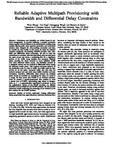
Fig. 4 shows the 10-th layer of capillary routing between a pair of end nodes on a network with 180 nodes and 1374 links. Links not carrying traffic are not shown. The solid lines of the diagram represent 55 bottleneck links belonging to one of the 10 layers. The dashed lines represent a min-cost solution of the remaining flow not enclosed in bottlenecks after the 10-th layer. There could be several tens of additional routing layers until complete capillarization is achieved.
links: nodes: layers: bottlenecks: remaining: 1: 2: 3: 4: 5: 6: 7: 8: 9: 10:
1374 180 10 55 155
of receptions by sinks increase proportionally in respect to each node’s flow-out coefficient (either positive or negative). The multi-source/multi-sink problems arise since the LP problem at each successive layer is obtained by complete removal of the bottlenecks from the previous LP problem. By removing the bottlenecks we adjust correspondingly the flow-out coefficients of the adjacent nodes (to respect the flow conservation rule) and thus possibly produce new sources and sinks in the network. Except for the unicast problem of the first layer, the successive layer problems do not belong in general to the simple class of “network linear programs” [Fourer03].
1.00000 0.50000 0.20000 0.16667 0.14286 0.11111 0.10714 0.10000 0.09524 0.08571
+1.5 +1.5
Fig. 4. Routing pattern of layer 10 built by the capillary routing algorithm on a network sample with 150 nodes
+2 +1 +1
–1
–4/3
–1
Although the described LP process is completely valid, it is numerically instable. The precision errors propagating through the layers of capillary routing reach noticeable sizes and, when dealing with tiny loads, result in infeasible LP problems. We have found a different, stable LP method which maintains the values of parameters and variables in the same order of magnitude at all times. Instead of decreasing the maximal value of loads of the links, the routing path is discovered by solving max flow problems defined by the flow-out coefficients at each node. Initially only the peer nodes have non-zero flow-out coefficients: +1 for the source and –1 for the sink (Fig. 5 and Fig. 6).
Fig. 5. Initial problem with one source and one sink node
+2/3
+0.5
2.2. Numerically stable version
+1
+2
+1.5
–2
–2
Fig. 6. Maximize the flow, fix the new flow-out coefficients at the nodes and find the bottleneck links (layer 1, F 1 = 2 )
Fig. 7. Remove the bottleneck links from the network and adjust the flow-out coefficients at the adjacent nodes
At each subsequent layer (Fig. 7 to Fig. 10) we have a bounded multi-source/multi-sink problem: a uniform flow from a set of sources to a set of sinks, where all rates of transmissions by sources and all rates
–4/3
–1 –3 Fig. 8. Maximize the flow in the new subproblem, fix the new flow-out coefficients at the nodes and find the new bottlenecks (layer 2, F 2 = 1.5 )
Fig. 9. Again remove the bottleneck links from the network and adjust correspondingly the flow-out coefficients at the adjacent nodes
Fig. 10. Maximize the flow in the obtained new problem, fixing the new resulting flow-out coefficients at the nodes and find the new bottlenecks (layer 3, F3 = 4/3)
We define the bounded multi-source/multi-sink problem at layer l by the sets of nodes and links and by the flow-out coefficients for sources and sinks (all indexed with an upper index l) as follows: - set of nodes N l , - set of links (i, j ) ∈ Ll , where i ∈ N l and j ∈ N l , - flow-out coefficients f i l for all i ∈ N l - at layer l the max-flow solution yields the flow increase factor F l and the set of bottlenecks B l , where B l ⊂ Ll Then, the equations for computing the sets N l +1 , Ll +1 and the flow-out coefficients f l +1 of the next layer are as follows: (1) - N l +1 = N l l +1 l l (2) - L =L −B - f jl +1 = f jl ⋅ F l + ∑ (+1) + ∑ (−1) (3) ( i , j )∈B l
( j , k )∈B l
add 1 for each subtract 1 for each incoming bottleneck outgoing bottleneck link (i, j) link (j, k)
After a certain number of applications of the maxflow objective with corresponding modifications of the problem, we will finally obtain a network having no source and sink nodes. At this point the iteration stops.
At each layer, after minimizing the maximal load of links, the bottlenecks of the layer are discovered in a bottleneck hunting loop. At each iteration of the hunting loop, we minimize the load of the traffic over all links having maximal load and being suspected as bottlenecks. Links not maintaining their load at the maximum are removed from the suspect list. The bottleneck hunting loop stops if there are no more links to remove.
10
9
1 layer
Fig. 12. A max-flow solution with the flow increase factor of 4/3, containing four maximally loaded candidate links {a, b, d, e}
10
8
–2
100
layer
–2
1000
layer
Fig. 11. An example of a bounded multi-source/multisink problem (obtained during construction of the capillary routing from a network with one source and one destination node)
In this example the two bottlenecks are found in two iterations. For capillary routing layers built simultaneously on 200 independent network samples each with 300 nodes (in average 2,555.7 links per network), Fig. 15 shows the decrease in the number of suspected links during the bottleneck hunting loop of each capillary routing layer from 1 to 10.
7
–1.5
Fig. 14. Cost reduction applied to the three fully loaded links of Fig. 13 reduces the load of another suspected link a, and the true bottleneck links are {b, e}.
layer
e
Fig. 13. Cost reduction applied to four fully loaded links of Fig. 12 reduces the load of suspected link d, and the suspect list is now {a, b, e}.
–2
6
–1.5
d c
–2
layer
b a
4/3
e
5
2/3 4/3
–2
d c
layer
4/3
–2
b
4
2/3
+1
a
3
+1
c
4/3
layer
+1
e
d
a
2/3 4/3
2
In the example of Fig. 11 with three transmitting nodes and two receiving nodes, the flow can be proportionally increased at most by a factor of 4/3 and the bottleneck links are among four maximally loaded suspected links {a, b, d, e}, marked in Fig. 12 by thick dashes.
4/3
layer
2.3. Bottleneck hunting loop
b
1/3 4/3
1
The max-flow approach proves to be very stable, because it maintains all values of variables and parameters in the same order of magnitude (even for very deep layers with tiny loads) and also because it enables us to detect and correct errors in the flow-out coefficients of the LP problem generated for the next layer of capillary routing. In the next subsection we show how to identify bottlenecks after the max-flow solution of the capillary routing layer is found.
1/3 4/3
layer
i =1
2/3 4/3
layer
(i, j ) ∈ B l of layer l is the initial single unit of flow divided by the product of the flow increase factors F i (where 1 ≤ i ≤ l ) of the present and all preceding layers: 1 where l is the ri , j = l (4) layer for which i l ∏ F (i, j) ∈ B
In the example of Fig. 12 the sum of loads of all four suspected links can be minimized (by an LP objective) to 3 (see Fig. 13). Now only three links {a, b, e}, marked by thick dashes, continue to maintain the maximal load. The sum of loads of three remaining suspected links can be further reduced to 2 (see Fig. 14). These two remaining links {b, e}, marked by thick dashes, maintained the maximal load at all times and are the true bottleneck links since the sum of their loads cannot be further reduced.
Average number of suspected links
All links followed by the flow in the capillary routing are enclosed in bottlenecks of one of the layers. In order to restore the original proportions of the flow, the flow increases, induced by the preceding max-flow solutions must all be compensated. The true value of flow ri , j traversing the bottleneck link
Iterations of the hunting loop (from 1 to 14 up to 23) for each of the first 10 layers of capillary routing
Fig. 15. Decrease of the number of suspected links during the bottleneck hunting loop of each of 10 capillary routing layers
At the end of each hunting loop (from 14 to 23 iterations) the suspect list consists of only true bottleneck links, in average between 5.9 and 9.9 bottlenecks per network.
3. Redundancy Overall Requirement (ROR) The definition and equations of ROR are given in subsection 3.1. Computation of transmission FEC block size as a function of the packet loss rate p is presented in subsection 3.2. Equation of ROR for a particular case of very large FEC blocks is presented in subsection 3.3.
3.1. Definition of ROR We assume a combination of a small static tolerance of the media stream to weak failures, with a dynamically added adaptive FEC for combating serious failures exceeding the tolerable packet loss rate. For a given routing pattern, ROR is defined as the sum of all transmission rate overheads required from the sender for combating each non-simultaneous link failure in the route. For example, if the communication footprint consists of five links, and in response to each individual link failure the sender increases the packet transmission rate by 25%, then the ROR coefficient will be equal to the sum of these five FEC transmission rate increases, i.e. ROR = 5 ⋅ 25% = 1.25 . If P is the usual packet transmission rate and Pl is the increased rate of the sender, responding to the failure of a link l ∈ L , where L is the set of all links, then: ⎞ ⎛P ROR = ∑ ⎜ l − 1⎟ (5) ⎠ l∈L ⎝ P Let us consider a long communication, and let D be the total failure time of a single network link during the whole duration of the communication. D is the product of the average duration of a single link failure, the frequency of a single link failure and the total communication time. According to equation (5): ⎛P ⎞ D ⋅ P ⋅ ROR = D ⋅ P ⋅ ∑ ⎜ l − 1⎟ (6) P ⎝ ⎠ l∈L = ∑ (D ⋅ Pl − D ⋅ P ) (7) l∈L
Assuming one single link failure at a time and a uniform probability and duration of link failures, according to equation (7), D ⋅ P ⋅ ROR is the number of adaptive redundant packets that the sender actually needs to transmit in order to compensate for all network failures occurring during the total communication time. Therefore ROR is a routing coefficient for computing the overall number of required redundant packets. Redundant packets are injected into the original media stream for every block of M source packets. During streaming, M is supposed to stay constant.
However, the number of redundant packets for each block of M media packets is variable, depending on the conditions of the erasure channel. The M source packets with their related redundant packets form a FEC block. By FEC p we denote the FEC block size chosen by the sender in response to a packet loss rate p. We assume that by default the media is streamed in FEC blocks of length of FECt such that the flow has a static tolerance to weak losses 0 ≤ t < 1 . When the loss rate p measured at the receiver is about to exceed the tolerable limit t, the sender increases its transmission rate by injecting additional redundant packets. The random packet loss rate, observed at the receiver during the failure time of a link in the communication path, is the portion of the traffic still being routed toward the faulty link. Thus, a complete failure of a link l carrying a relative traffic load of 0 ≤ r (l ) ≤ 1 according to the routing pattern, produces at the receiver a packet loss rate equal to the same relative traffic load r (l ) . Equation (5) for ROR can thus be re-written as follows: ⎛ FECr (l ) ⎞ ⎜⎜ − 1⎟⎟ ∑ (8) ROR = l∈L | t ≤r ( l )