to minimize both tree and recovery costs, while finding an RST is very challenging. ... Hard and inapproximable within k, which is the number of destination ... control plane and data plane in a network and allows the .... SDN-C can find the best.
Reliable Multicast Routing for Software-Defined Networks Shan-Hsiang Shen* , Liang-Hao Huang* , De-Nian Yang* and Wen-Tsuen Chen*† *
Institute of Information Science, Academia Sinica, Taipei, Taiwan of Computer Science, National Tsing Hua University, Hsinchu, Taiwan
† Department
Email: {sshen3, lhhuang, dnyang, chenwt}@iis.sinica.edu.tw Abstract—Current traffic engineering in SDN mostly focuses on unicast. By contrast, compared with individual unicast, multicast can effectively reduce network resources consumption to serve multiple clients jointly. Since many important applications require reliable transmissions, it is envisaged that reliable multicast plays a crucial role when an SDN operator plans to provide multicast services. However, the shortest-path tree (SPT) adopted in current Internet is not bandwidth-efficient, while the Steiner tree (ST) in Graph Theory is not designed to support reliable transmissions since the selection of recovery nodes is not examined. In this paper, therefore, we propose a new reliable multicast tree for SDN, named Recover-aware Steiner Tree (RST). The goal of RST is to minimize both tree and recovery costs, while finding an RST is very challenging. We prove that the RST problem is NPHard and inapproximable within k, which is the number of destination nodes. Thus, we design an approximate algorithm, called Recover Aware Edge Reduction Algorithm (RAERA), to solve the problem. The simulation results on real networks and large synthetic networks, together with the experiment on our SDN testbed with real YouTube traffic, all manifest that RST outperforms both SPT and ST. Also, the implementation of RAERA in SDN controllers shows that an RST can be returned within a few seconds and thereby is practical for SDN networks. Keywords—SDN, multicast, traffic engineering, reliable transmissions
I.
I NTRODUCTION
Software-defined networking (SDN) is a new architecture that enables flexible network resources management to support a huge amount of data delivery [1]. It separates the control plane and data plane in a network and allows the control plan to be programmable for effectively optimizing the network resources allocation. OpenFlow [2] in SDN consists of two main components: controllers (SDN-Cs) and forwarding elements (SDN-FEs). A controller takes control plane from switches and installs the corresponding forwarding policies through secured interfaces. Forwarding elements in switches are flexible to support various forwarding rules for different traffic. Compared with the traditional distributed shortest-path routing, SDN enables a centralized computation on unicast routing for traffic engineering [3] to improve the network throughput. Nevertheless, multicast traffic engineering for SDN has attracted much less attention in the literature. Multicast is designed to deliver contents to a large number of destinations. Compared with unicast, multicast
can effectively reduce the bandwidth consumption in backbone networks by around 50% [4], because it exploits a tree, instead of disjoint paths, to connect the source and destinations; thus, it avoids unnecessary traffic duplication in intermediate nodes. For multimedia traffic, previous studies [5] further pointed out that multicast is able to release the load in the network links and I/O at the video servers, while VCR-like interactivity required by videoon-demand services can also be supported in multicast [5], [6]. Current multicast routing standards, such as PIMSM [7], connect the source and a group of destinations by a shortest-path tree. Traffic engineering is difficult to be supported in a shortest-path tree since the path from the root (i.e., source) of the tree to each destination is still the shortest path. Since the path to each destination is calculated individually, the shortest-path tree loses many good opportunities to reduce the bandwidth consumption by aggregating more edges in the paths, i.e., letting the paths share more common edges. By contrast, a Steiner tree (ST) [8] in Graph Theory is more promising because it minimizes the number of edges in a tree required for a multicast group. Nevertheless, ST is not adopted in the current Internet since it is computationally intensive and difficult to be deployed in a distributed manner. Fortunately, with the emergence of SDN, it now becomes a feasible approach to reduce the bandwidth consumption of multicast traffic. Nevertheless, even the multicast delivery is equipped with such a power theoretical tool to minimize the network resources consumption, users will not choose the multicast delivery option if reliable transmissions are not provided in multicast. Nowadays, many applications rely on reliable transmissions, even multimedia applications such as YouTube, Microsoft Smooth Streaming, and MPEG DASH [9]. To support reliable transmissions in multicast, source-based reliable multicast [10] is first introduced to directly recover the loss packets from the source, but it suffers from the scalability problem since the source is inclined to be overwhelmed because it needs to provide loss recovery for a large number of destinations [11]. To effectively address this crucial issue, a hierarchical architecture [11], [12] with on-tree recovery nodes placed between the source and the destinations is proposed to facilitate local loss recovery. The idea is similar to the web and multimedia cache/proxy servers widely deployed today, with the goal to facilitate local services and avoid load concentration on the source node. However, it is not necessary to deploy an explicit high-performance server with a large storage for a recovery
node, because a recovery node only needs to temporarily cache a tiny window of packets, instead of the whole files in a proxy server. Therefore, reliable multicast has been implemented in the current routers [13], [14], and it is important for a multicast tree to choose and span some recovery nodes in order to facilitate effective loss recovery. It is envisaged that a lower recovery cost will be reduced if a destination is close to its recovery node, but in this case more recovery nodes are necessary to be included in the tree. On the other hand, if the source is the only recovery node, the source implosion problem will limit the scalability of multicast. For SDN networks, it is necessary for a multicast tree to span suitable recovery nodes for local loss recovery and minimize the recovery load and the corresponding traffic, but the Steiner-tree routing does not consider the selection of the recovery nodes and thus is difficult to facilitate local loss recovery, especially when some network nodes are not able to play the role as the recovery nodes. In the worst case, the Steiner tree may not be able to span any recovery nodes. Therefore, it is desired to design a new algorithm to jointly find the routing of a multicast tree and the selection of recovery nodes for multicast traffic. In this paper, therefore, we propose a new reliable multicast tree for SDN, called Recover-aware Steiner Tree (RST). Given the source and destinations in a multicast group, together with the set of candidate recovery nodes in the network and a non-negative integer r, the RST problem aims to find a tree to 1) connect the source and the destinations and 2) span at most r recovery nodes as intermediates in the tree for local loss recovery. The objective is to minimize the summation of the tree cost and total recovery cost, while the tree cost is the total cost of all edges in the tree [8]. To support a large number of destinations, it is encouraged to facilitate local loss recovery by selecting the recovery nodes close to the destinations. Therefore, the recovery cost of a destination v is the cost of the path from its local proxy (i.e., recovery node) u to v in the tree [11], and a smaller recovery cost implies lower retransmissions delay and bandwidth consumption. Similarly, the recovery cost of a recovery node u is the cost of the path from the source s to u in the tree. Parameter r plays an important role as the tuning knob. By setting a larger r, more recovery nodes can be selected in the tree to effectively decrease the recovery cost, but the temporarily caching overhead also increases. SDN-C can find the best tradeoff by setting different r to find the desired solution. Compared with the shortest-path tree, the RST is envisaged to allocate the network resources more efficiently since both the routing and the selection of the recovery nodes are considered jointly. Compared with the ST, finding the RST is more challenging due to the selection of recovery nodes and its impacts on routing. The ST problem is NPHard but can be approximated within ratio 1.55 [15], and it is thus in APX of complexity theory. It means that there exists an approximation algorithm for ST that can find a tree with the total tree cost at most 1.55 times of the optimal solution. However, the RST problem is more difficult. We prove that the problem is NP-hard but not able to be approximated within k, which is the number of destinations in a multicast group. To solve RST efficiently, we propose a k-approximation algorithm, named Recover Aware Edge Reduction Algorithm (RAERA), which can be deployed
in SDN controllers. RAERA is divided into two phases, Tree Routing Phase and Recovery Selection Phase, to minimize both tree and recovery costs. Because no (k 1−ε )approximation algorithm exists in RST for an arbitrarily small ε > 0, RAERA achieves the best approximation ratio. The rest of this paper is organized as follows. Section II summarizes the literature. Section III presents the problem formulation and the hardness result. We design a k-approximation algorithm in Section IV, and Section V presents the results of our algorithm in a small real network, large synthetic networks, and our SDN testbed. Finally, we conclude this paper in Section VI. II.
R ELATED W ORKS
Previous works on SDN have extensively explored the issues on traffic engineering for unicast traffic in SDN. Agarwal et al. [3] considered unicast traffic engineering in the case where a SDN-C controls only a few SDNFEs in the network, and the rest of the network adopts a standard routing protocol, such as OSPF. The merits of traffic engineering brought by only a limited number of SDN-capable nodes are demonstrated. Mckeown et al. [2] pointed out that OpenFlow can be deployed with heterogeneous switches. Sushant et al. [16] shared their experience of SDN development for the private WAN of Google Inc. Qazi et al. [17] proposed a new system design in SDN for the middleboxes. Furthermore, Mueller et al. [18] presented a cross-layer framework in SDN, which integrates a novel dynamic traffic engineering approach with an adaptive network management. Nevertheless, multicast traffic engineering has not been addressed in the above works. Current multicast routing standards [7] employ the shortest paths provided by unicast routing protocols [19] to build shortest-path trees for distributed multicast routing. However, in spite of simple construction, the shortestpath tree is difficult to effectively reduce the bandwidth consumption. By contrast, the Steiner tree [8] is able to find a tree with the minimum cost. Nevertheless, the Steiner tree is not adopted in the current Internet because it is computationally intensive and difficult to be constructed in a distributed manner. To address this issue, overlay Steiner trees [20], [21] for P2P environments were proposed as an alternative way. Those approaches find the P2P clients to be directed connected by a path in an overlay tree. However, the path between any two P2P clients is still the shortest path in the network, and the routing of the P2P tree is thereby difficult to be optimized. Reliable transmissions for loss packet recovery are crucial in many Internet applications, even the multimedia streaming applications such as YouTube, Microsoft Smooth Streaming, and MPEG DASH [9]. The source node is in charge of the lost packet recovery in TCP for unicast traffic. Nevertheless, it has been manifested that this simple sourcerecovery strategy is not scalable [11], [12] for multicast to support a large number of destinations, because the source node will be overwhelmed by the acknowledgement from the destinations and the required recovery traffic. To effectively address this issue, by exploiting the idea of local services via proxy servers [22], a hierarchical architecture [11], [12] with on-tree recovery nodes placed between the source and the destinations is proposed to
facilitate local loss recovery, while the deployment of the recovery nodes has not been considered as an issue in the previous works since the recovery nodes only need to support temporary caching, and the literature thus mostly focused on the development of a low-overhead protocol with acknowledgement (ACK) or negative acknowledgement (NAK). Specifically, Reliable Multicast Transport Protocol II (RMTP-II) [11] properly designed the interval between subsequent ACKs to reduce the number of ACK messages from a destination to its recovery node, or from a child recovery node to its parent recovery node. Pragmatic General Multicast (PGM) [12] proposed NAK elimination and NAK suppression to further reduce the number of NAK messages delivered. NACK-Oriented Reliable Multicast (NORM) Transport Protocol [23] incorporated forward error corrections (FEC). Without a reliable multicast scheme deployed in the SDN network, it is envisaged that most multicast applications will still choose the unicast delivery, which incurs a huge amount of waste in the network resources due to unnecessary traffic duplication. The above reliable multicast approaches assume that the recovery nodes have been allocated in a shortest-path tree and thus focus on minimizing the number of ACK and NAK messages accordingly. However, to support reliable multicast, it is necessary for a multicast tree to span suitable recovery nodes for local loss recovery and minimize the recovery load and the corresponding traffic, but the Steinertree routing does not consider the selection of the recovery nodes and thus is difficult to facilitate local loss recovery, especially when only a few network nodes are able to play the role as the recovery nodes. Therefore, it is desired to design a new algorithm to jointly find the routing of a multicast tree and the selection of recovery nodes for multicast traffic.
III.
P ROBLEM D ESCRIPTION
A. Problem Formulation In this paper, we propose a new multicast tree for SDN, called Recover-aware Steiner Tree (RST). RST T aims to minimize the tree cost and the recovery cost for multicast traffic. In addition to finding the set of edges spanning the source s and the destination set D, it is necessary to identify at most r recovery nodes in a set R in T . More specifically, consider a directed graph G(V, E), where V and E denote the set of nodes and directed edges, respectively. Each edge e ∈ E is associated with a cost1 c(e) : E → R+ , where R+ is a set of positive real numbers. To find the recovery cost, we first define the recovery path P for each destination node in D and each recovery node in R as follows. Definition 1: For each node v in D ∪ R, the parent recovery node par(v) of v is a node u ∈ R ∪ {s} in the path from s to v in T , such that there is no other recovery node between u and v in the path. The path from par(v) to v in T is called the recovery path Pv of v. The total cost 1 In wired networks, packets are lost and dropped usually due to network congestion, which are difficult to be predicted and avoided. Thus, in traffic engineering [24], a congested link is assigned a higher cost so that it will have a smaller chance to be selected in a routing algorithm for a new traffic connection. In other words, a link with more packet losses and experiencing a larger delay will be assigned a higher cost.
of edges in the recovery path P is called the recovery cost2 w(Pv ) of v. We define the tree cost and the recovery cost and then formulate the RST problem as follows. Definition 2: The cost of the ordinary traffic is represented by the tree cost c(T ), which is the sum of the edge cost c(e) for every edge e ∈ T . The cost and the recovery delay of the recovery traffic are represented by the recovery cost w(T ), which is the sum of the recovery cost w(Pv ) for every node v ∈ D ∪ R. Definition 3: Given G(V, E), a destination node set D ⊆ V , a candidate recovery node set C ⊆ V , a nonnegative integer r, and a non-negative value α, the Recoveraware Steiner Tree (RST) problem is to find a recovery set R ∈ C with |R| ≤ r and a tree T spanning s and D such that c(T ) + αw(T ) is minimized. In the RST problem, SDN-C can flexibly adjust the tradeoffs between the local storage overhead and the recovery cost w(T ) by testing different r. With a large r, more nodes in T will be involved to temporarily store the multicast traffic for loss recovery, but the recovery cost can be effectively reduced. In addition, SDN-C can flexibly tune the weight α according to the network status. If the network is heavily loaded, it is necessary to assign a larger α such that the assignment of R will play a more important role in order to effectively reduce the recovery cost. Since the RST problem addresses both the routing of a tree and the section of recovery nodes, it is envisaged that the RST problem is more difficult than the traditional ST problem. As follows, we show that the RST problem is very challenging in complexity theory by proving that it is NP-Hard and not able to be approximated within |D|c for every c < 1. B. Hardness result The RST problem is NP-Hard because it equals to the ST problem when α is 0. In other words, the ST problem is a special case of the RST problem. However, the RST problem is much more challenging because the ST problem can be approximated within ratio 1.55 [15] and is thus in APX in complexity theory, but we find out that the RST problem is much more difficult to be approximated. The following theorem proves that the RST problem cannot be approximated within |D|c for every c < 1, by a gapintroducing reduction from the Set Cover problem. Theorem 1: For any ǫ > 0, there exists no |D|1−ǫ approximation algorithm for the RST problem with α > 0, assuming P 6= NP. Proof: We prove the theorem with the gap-introducing reduction from the Set Cover problem. For a bipartite graph 2 When a packet loss occurs, a recovery node can (1) retransmit the packet to individual destination not receiving the packet [11], (2) multicast the packet again to all downstream nodes [11] in its subtree, or (3) subcast the packet only to the downstream nodes not receiving the packet [12]. For the last scheme, the recovery cost is difficult to be evaluated as a static term in the objective function of the RST problem, since the set of downstream nodes not receiving a packet varies from time to time. Therefore, we first explore the first two schemes accordingly. We present the problem formulation of the first scheme and show that the second scheme is a special case of the problem formulation by setting α = 0. The advantage is that the recovery cost can also represent the recovery delay in this case.
(X, Y, E), the Set Cover problem aims to find out whether there exists a k-node subset of X that can cover all nodes in Y . For an instance of the Set Cover problem, we build an instance of the RST problem on G(V, E), such that • if (X, Y, E) has a k-node subset of X covering all nodes in Y , then OPT(G) ≤ (α + 1)(k + 1)|D|, and • if (X, Y, E) does not have a k-node subset of X covering all nodes in Y , then OPT(G) > (α + 1)(k + 1)|D|2−ǫ , where OPT(G) is the optimal solution of G for the RST problem. We first detail how to build the instance of the RST problem from the Set Cover problem. For any given k and (X, Y, E), we construct a new graph G with V including X and |Y |p , copies of Y , where p is the smallest integer α such that p ≥ 1+log(α+1)+log(k+1)−log − 1, and the base ǫ of logarithm is |Y |. One additional source node s is added to V and connected to each node of X. The cost of each edge from s to X is set to |Y |p+1 , and the cost of each edge from X to each copy of Y is set to 1. Destination set D is set to all nodes in the |Y |p copies of Y , and r is set to k. Candidate recovery node set C is set to V . If (X, Y, E) has a k-node subset A of X covering all nodes in Y , we are able to find a tree rooted at s with the edges from s to all nodes in A and the edges from all nodes in A to every node of all copies of Y , and R is set as A. Thus, tree T is a feasible solution of the RST problem because the source s is connected to every node in D via T . It can act as an upper bound of the RST problem in G. Since |Y |p+1 = |D|, the tree cost c(T ) is k|D| + |D|, and the recovery cost w(T ) is k|D| + |D|. Therefore, OPT(G) ≤ (k|D| + |D|) + α(k|D| + |D|) = (α + 1)(k + 1)|D|. On the other hand, if (X, Y, E) does not have a k-node subset of X covering all nodes in Y , then the optimal tree must contain at least k + 1 nodes in X, and for each copy of Y , at least one vertex connects to a nonrecovery node, leading to a much higher recovery cost (i.e., at least |D||Y |p ) due to a longer recovery path from every node in D to the source s. Hence, OPT(G) > α|D||Y |p = (α + 1)(k + 1)|D||Y |p−(log(α+1)+log(k+1)−log α) = (α + p−(log(α+1)+log(k+1)−log α) p+1 = (α+1)(k+ 1)(k+1)|D|(|Y |p+1 ) 1+log(α+1)+log(k+1)−log α 2− p+1 1)|D| ≥ (α + 1)(k + 1)|D|2−ǫ . Since ǫ can be arbitrarily small, for any ǫ > 0, there is no |D|1−ǫ approximation algorithm for the RST problem, assuming P 6= NP. The theorem follows.
routing of the tree with εu,v = 1 for every edge eu,v in T can be constructed with the union of the paths from s to all destination nodes in D To find the recovery cost, let binary variable ρv denote if v is a recovery node in T , and let κv denote the recovery cost of each node v, κv ≥ 0. The objective function of the RST problem is as follows. " # X X X min cu,v εu,v + α κd + ρv κv , eu,v ∈E
d∈D
v∈C−D
where cu,v = c(eu,v ). The first and second terms are the tree cost and the recovery cost, respectively. The second term includes the recovery P costs for the destinations and the recovery nodes, while ρv κv ensures that only the v∈C−D
recovery cost for each selected recovery node (i.e., ρv = 1) will be incorporated. However, the above objective function is not linear because both ρv and κv are decision variables. To address this issue, we introduce a new decision variable χv to represent the recovery cost of each recovery node v, χv ≥ 0, while χv of every non-recovery node v will be enforced to 0 explained later in this section. Now the objective function of the MILP formulation for the RST problem is " # X X X min cu,v εu,v + α κd + χv . eu,v ∈E
d∈D
v∈C−D
If the tree T contains any cycle, T is not optimal since we are able to remove at least one edge from the cycle to reduce the objective value, and T thereby ensures that there still exists only one path from s to every destination node d in D. To find εu,v from πd,u,v , together with ρv , κv , χv , our MILP formulation includes the following constraints. P
v∈N Ps
u∈Nd
πd,s,v −
P
πd,v,s = 1, ∀d ∈ D,
(1)
πd,u,d − πd,d,u = 1, ∀d ∈ D, u∈Nd P P πd,v,u = πd,u,v ,
(2)
v∈N Ps
v∈Nu
v∈Nu
∀d ∈ D, ∀u ∈ V, u 6= d, u 6= s, πd,u,v ≤ εu,vP , ∀d ∈ D, ∀eu,v ∈ E, ρu ≤ r,
(3) (4) (5)
v∈V −{s}
C. Mixed Integer Linear Programming In the follows, we design a Mixed Integer Linear Programming (MILP) formulation for the RST problem, and the formulation can collaborate with any commercial MILP solver, such as IBM ILOG CPLEX [25], to find the optimal solutions for small instances of the problem. Specifically, let Nv denote the set of neighbor nodes of v in G, and u is in Nv if eu,v is an edge from u to v in E. Let s denote the source of the multicast group, and D denote the destination set. The output tree T needs to ensure that there is only one path in T from s to every node in D. To achieve this goal, our problem includes the following binary decision variables. Let binary variable πd,u,v denote if edge eu,v is in the path from s to a destination node d. Let binary variable εu,v denote if edge eu,v is in T . Intuitively, when we are able to find the path from s to each destination node d with πd,u,v = 1 on every edge eu,v in the path, the
cu,v εu,v − (2 − εu,v − ρu ) L ≤ κv , ∀eu,v ∈ E, κu + cu,v εu,v − (1 − εu,v + ρu ) L ≤ κv , ∀eu,v ∈ E, κu − (1 − ρu ) L ≤ χu , ∀u ∈ V, ρu = 0, ∀u ∈ V − C − {s}.
(6) (7) (8) (9)
Path and Tree Routing Constraints. The first three constraints, i.e., (1), (2), and (3), are the flow-continuity constraints to find the path from s to every destination node d in D. More specifically, s is the flow source, i.e., the source of the path to every destination node d, and constraint (1) states that the net outgoing flow from s is one, implying that at least one edge es,v from s to any neighbor node v needs to be selected with πd,s,v = 1. Note that decision variables πd,s,v and πd,v,s are two different variables because the flow is directed. On the other hand, every destination node d is the flow destination, and constraint (2) ensures that the net incoming flow to d is one, implying that at least one edge eu,d from any neighbor node
u to d must be selected with πd,u,d = 1. For every other node u, constraint (3) guarantees that u is either located in the path or not. If u is located in the path, both the incoming flow and outgoing flow for u are at least one, indicating that at least one binary variable πd,v,u is 1 for the incoming flow, and at least one binary variable πd,u,v is 1 for the outgoing flow. Otherwise, both πd,v,u and πd,u,v are 0. Note that the objective function will ensure that πd,v,u = 1 for at most one neighbor node v to achieve the minimum cost. Constraint (4) is formulated to find the routing of the tree i.e., εu,v . It states that εu,v must be 1 if edge eu,v is included in the path from s to at least one d, i.e., πd,u,v = 1. The tree T is the union of the paths from s to all destinations. Recovery Allocation Constraints. Constraint (5) states that at most r recovery nodes are selected. The last three constraints are the most crucial ones in order to linearize the objective function and construct the MILP formulation, which enables us to find the optimal solution of the RST problem. More specifically, we let L = c(G) as the total cost of all edges in the network G. For each recovery node u (with ρu = 1) and each incident tree edge eu,v of u in T (with εu,v = 1), constraint (6) now becomes cu,v εu,v ≤ κv , enforcing that the recovery cost of each child node v of the recovery node u is at least cu,v εu,v . Note that for any incident edge eu,v of a node u not in T (i.e., εu,v = 0), the left-hand-side (LHS) of constraint (6) will become smaller than 0 and thus lead to no restriction on κv in the righthand-side (RHS). Similarly, if u is not a recovery node, LHS of constraint (6) will also become smaller than 0. In other words, constraint (6) is specifically designed for each recovery node u and its incident edge eu,v in T . By contrast, for any other non-recovery node u in T (with ρu = 0) and its incident edge eu,v of u in T (with εu,v = 1), constraint (7) becomes κu + cu,v εu,v ≤ κv , which ensures that the recovery cost κv for the child node v of u is at least κu + cu,v εu,v , and constraint (7) will not impose any restriction on κv for any other cases, similar to constraint (6). Since there is only one path in T from its recovery node to each destination node d, the hop-byhop enforcement from κu to κv for each edge eu,v in T guarantees that recovery cost κd of d is at least the total cost of its recovery path. Constraint (8) states that χu is at least κu for each recovery node u. The final constraint ensures that only s and the nodes in C are capable to act as the recovery nodes. IV.
A LGORITHM D ESIGN
denote the cost of the longest shortest path from s to any destination d in D in the tree. RAERA iteratively re-routes a destination node on the solution tree T (VT , ET ) to reduce the tree cost. We calculate the shortest path from all the other nodes on the tree to a destination d, and pick up a re-routing path that leads to the maximal reduction of the tree cost. Therefore, the re-routing path can connect to a nearby end-to-end path from s to another destination to aggregate the two paths. We restrict a destination from re-routing to the end-to-end paths that it has connected to in earlier iterations. More importantly, the re-routing path needs to include at least one candidate recovery node in C to facilitate local loss recovery. In addition, the cost of the end-to-end path from s to d in the new tree cannot exceed M , to avoid generating a path longer than the depth of the original shortest-path tree. The re-routing process continues until the tree cost cannot be further reduced. Afterwards, Recovery Selection Phase is a dynamic programming algorithm to select the recovery nodes from C for minimizing the recovery cost. For each node v ∈ VT , let Tv be the subtree of T rooted at v. Let Rv be a recovery set on Tv , and the recovery cost of Tv with respect to Rv is denoted by w(Tv , Rv ). The dynamic programming algorithm finds the optimal recovery sets for two cases: v is selected in Rv . If v is not selected in Rv , the algorithm will assign some ancestor nodes in T as the parent recovery node of v later. We call a recovery set Rv on Tv is type I if v ∈ / R. By contrast, Rv belongs to type II if v ∈ Rv . Given the recovery set Rv , a node u (u 6= v) in D ∪ Rv is dominated by any node v if there is no other recovery node in Rv located in the path from v to u in Tv . For a non-negative integer x ≤ r and a positive integer k ≤ |D|, let σx,k (Tv ) denote the minimum recovery cost on Tv over all type I recovery set Rv (v is not in Rv ) with |Rv | ≤ x, such that v exactly dominates k nodes in Rv ∪ D on Tv . Similarly, let τx (Tv ) denote the minimum recovery cost on Tv over all type II recovery set Rv with |Rv | ≤ x. It is worth noting that τx (Tv ) does not need to include a subscript k because the parent recovery node par(v) of v only needs to serve one node (i.e., v) in Tv . By contrast, it is necessary to associate k with σx,k (Tv ) to represent the case that the parent recovery node serves k nodes in Tv , while different k is examined in the algorithm to find the optimal set of recovery nodes after the whole tree T is processed. In addition, since the recovery costs σx,k (Tv ) and τx (Tv ) sum up only the costs of the edges on Tv , τx (Tv ) = min σx−1,k (Tv ) holds for x ≥ 1 when v ∈ C. 1≤k≤|D|
In the follows, we propose a k-approximation algorithm, called Recover Aware Edge Reduction Algorithm (RAERA), to find the routing of multicast tree and select the local recovery nodes for jointly minimizing the tree cost and recovery cost. Theorem 1 proves that no (k 1−ǫ )approximation algorithm for any ǫ > 0 for the RST problem, RAERA achieves the best approximation ratio. Due to space constraint, the pseudocode and online rerouting to support the dynamic join and leave of destinations are presented in [26].
Specifically, suppose v has child nodes u1 , . . . , uδv , where δv is the number of child nodes of v in T . Let L denote the set of leaf nodes in T , L ⊆ D. We let σx,k (Tv ) and τx (Tv ) as ∞ initially for every v ∈ VT − L, x, and k. Let Tvi be the subtree of Tv that contains v and the nodes on Tui . The following lemmas first find σx,k (Tvi ) and then derive σx,k (Tv ) from σx,k (Tvi ), while τx (Tv ) can be calculated from σx−1,k (Tv ) accordingly.
RAERA includes two phases: 1) Tree Routing Phase and 2) Recovery Selection Phase. The first phase starts from the shortest-path tree with root s and iteratively improves the tree to reduce the tree cost. More specifically, let M
Lemma 1: For each node v ∈ / L and its child nodes u1 , . . . , uδv in T , the following equations hold, 0 ≤ x ≤ r, 1 ≤ k ≤ |D|, and 1 ≤ i ≤ δv .
(i) If ui ∈ D, then σx,k (Tvi ) = ( if k = 1 and ui ∈ L, cvui if k = 1, ui ∈ C, and ui ∈ / L, τx (Tui ) + cvui σx,k−1 (Tui ) + k ∗ cvui if k > 1,
Based on Lemma 1 and Lemma 2, the dynamic programming algorithm in the second phase of RAERA minimizes the recovery cost in a bottom-up manner from the leaf nodes, and the following theorem proves that the minimum recovery cost can be obtained when s is reached.
when τx (Tui ) and σx,k−1 (Tui ) are not ∞.
Theorem 2: Given the routing of the tree T , the minimum recovery cost is min1≤k≤|D| σr,k (Ts ).
(ii) If ui ∈ / D, then σx,k (Tvi ) = � min{σx,1 (Tui ) + cvui , τx (Tui ) + cvui } σx,k (Tui ) + k ∗ cvui
if k = 1, if k > 1,
when σx,k (Tui ) and τx (Tui ) are not ∞. Proof: We examine the first case with ui ∈ D. For k = 1, if ui ∈ L, then σx,1 (Tvi ) = cvui holds since Tvi has only one edge. By contrast, if ui ∈ C and ui ∈ / L, ui needs to act as a recovery node when k = 1 since ui ∈ D; if ui does not act as a recovery node, there are at least two nodes (i.e., ui and some downstream destination) dominated by ui and thus contradict that k = 1. Therefore, w(Tui , Rui ) = τx (Tui ). Let Rvi = Rui be the recovery set on Tvi . When Rvi is a type I recovery set with v ∈ / Rvi , we have σx,1 (Tvi ) = τx (Tui ) + cvui if τx (Tui ) 6= ∞. When k > 1, ui cannot act as a recovery node. Let Rui be a type I recovery set on Tui with |Rui | ≤ x, and ui dominates k − 1 nodes since v dominates k nodes (i.e., ui is a destination). Therefore, w(Tui , Rui ) = σx,k−1 (Tui ) in this case. Let Rvi = Rui be a recovery set on Tvi , and Rvi is a type I recovery set with v ∈ / Rvi . Node v dominates ui ∈ D and k − 1 other nodes downstream two ui , and w(Tvi , Rvi ) = w(Tui , Rui )+k∗cvui = σx,k−1 (Tui )+k∗cvui holds. Therefore, we have σx,k (Tvi ) = σx,k−1 (Tui )+k∗cvui if σx,k−1 (Tui ) 6= ∞. The second case with ui ∈ / D is simpler than the first one. When k = 1, it is only necessary to pick up the smaller one of σx,1 (Tui ) and τx (Tui ) for deriving σx,k (Tvi ) since v has only one child node ui in Tvi . When k > 1, ui cannot act as a recovery node, and thus we derive σx,k (Tvi ) according to σx,k (Tui ). The lemma follows. Lemma 2: Suppose u1 , . . . , uδv are the child nodes of v ∈ VT . For 2 ≤ j ≤ δv , the following equality holds. σx,k (
j [
Tvi )
=
i=1
min {σx−x′ ,k−k′ ( ′
x ∈[0,x] k′ ∈[1,k]
j−1 [
Tvi ) +
i=1
σx′ ,k′ (Tvj )}.
Proof: Given x′ ∈ [0, x] and k ′ ∈ [1, k], let R1 (R2 ) Sj−1 be a type I recovery set on i=1 Tvi (Tvj ) such that |R1 | ≤ x−x′ (|R2 | ≤ x′ ), and v dominates k−k ′ (k ′ ) nodes, Sj−1 respectively. Since v is the unique common node of i=1 Tvi and Sj Tvj , v dominates (k −k ′ )+k ′ = k nodes in i=1 Tvi . Hence Sj R1 ∪R2 is a type I recovery set on i=1 Tvi with |R1 ∪R2 | ≤ Sj−1 x and v dominating k nodes. Then w( i=1 Tvi , R1 ) + Sj Sj w(Tvj , R2 ) = w( i=1 Tvi , R1 ∪ R2 ) = σx,k ( i=1 Tvi ). ′ ′ Because all possible x and k are fully examined, we have j j−1 [ [ σx,k ( Tvi ) = ′min {σx−x′ ,k−k′ ( Tvi ) + σx′ ,k′ (Tvj )}. i=1
x ∈[0,x] k′ ∈[1,k]
i=1
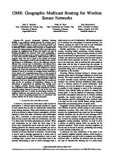
Proof: We prove the theorem by contradiction. Assume that the solution, i.e., min1≤k≤|D| σr,k (Ts ), is not optimal. There must exist ks such that σr,ks (Ts ) is not an optimal solution. According to Lemma 2, there exists i ∈ [1, δs ] with xi and ki such that σxi ,ki (Tsi ) is not optimal. Let v be the i-th child node of s, then according to Lemma 1, either σxi ,kv′ (Tv ) or τxi (Tv ) is not optimal for some kv′ . Since τxi (Tv ) can be represented by σxi −1,kv′′ (Tv ), we can find σxv ,kv (Tv ) that is not optimal for some xv and kv . After repeating above procedure, we can find a node u such that the order of u is before v, and σxu ,ku (Tu ) is not optimal for some xu and ku . Finally, we can find a node t whose child nodes are all in L and σxt ,δt (Tt ) is not optimal. According to Lemma 1 (i), we have σxt ,kt (Tti ) = ctui for 1 ≤ i ≤Pδt . Then according to Lemma 2, we have the minimum recovσxt ,δt (Tt ) = 1≤i≤δt ctui . However, P ery cost of tree Tt is exactly 1≤i≤δt ctui = σxt ,δt (Tt ), contradicting that σxt ,δt (Tt ) is not optimal. The theorem follows. Afterwards, the optimal recovery node can be selected by backtracking the above procedure. More specifically, let ks = arg min1≤k≤|D| σr,k (Ts ), and we then insert σr,ks (Ts ) as the LHS of Lemma 2 and derive (x∗ , k ∗ ) that minimizes the RHS. If k ∗ = 1 and uδs ∈ D − L for the last child node of s, we add uδs to R according to Lemma 1. / D, we add uδs to R when Similarly, if k ∗ = 1 but uδs ∈ σx∗ ,k∗ (Tsδs ) = τx∗ (Tuδs ) + cvuδs . The above procedure is repeated until all leaf nodes in L are processed. Example. Consider the following example in Fig. 1(a). Let G(V, E) be the network with the source node s, the destination set D = {1, 2, . . . , 12}, the candidate recovery set C = V − {1, 7, e, w, x}, and r = 3. The shortestpath tree with root s is shown in Fig. 1(b). Then Fig. 1(c) presents an example of Tree Routing Phase. If nodes 1 and 3 were re-routed to node w, then it could reduce the maximal tree cost. However w is not a candidate recovery node, and thus nodes 1 and 3 are re-routed to node u. Then node 4 is re-routed to node 5, and node 6 is re-routed to node v. Afterwards, node 8 and 9 are re-routed to node 10. Finally, node 7 is re-routed to node 8. Afterwards, Recovery Selection Phase is a dynamic programming algorithm to select recovery nodes from C to minimize the recovery cost. We illustrate how Recovery Selection Phase derives σx,k (T12 ), when 0 ≤ x ≤ 2 and 1 ≤ k ≤ 4. At the beginning, we find all σx,k (Tu ). According to Lemma 1 and 2, we have σ0,3 (Tu ) = σ1,3 (Tu ) = σ2,3 (Tu ) = 9 and τ1 (Tu ) = τ2 (Tu ) = 9. 1 Then we compute σx,k (T11 ). Since node u ∈ / D, according to Lemma 1 (ii), for 1 ≤ x ≤ 2, it follows that 1 ) = min{σx,1 (Tu ) + 5, τx (Tu ) + 5} = 14, and σx,1 (T11 1 1 1 σ0,3 (T11 ) = σ1,3 (T11 ) = σ2,3 (T11 ) = 9 + 3 ∗ 5 = 24. 1 Since σx,k (T11 ) = σx,k (T11 ), we get all σx,k (T11 ) and τ1 (T11 ) = 24, and τ2 (T11 ) = 14. Finally, we compute 1 ). Since node 11 is in D − L, σx,k (T12 ) = σx,k (T12
source non-destination destination 12 5
11 u
3
2
2 2 w 2 1 2 1
1
x
b
4
c 6
1
1 10
8
3
5
6
1
7 2 1
1
2 2
5
2
2
9
3 3
9
8 9
(a) Original network s
3 6 1
11 5 u 2 w 2 2
3 1
5 12 d 1 2
c
6
1
e 5
8
v
10
6 7
2 5
4 3
3
2
2 9 8
(b) Shortest-path tree with root s Fig. 1.
s
1 8 b 1 6 c 1 3 11 d e 3 5 1 10 u 1 v 6 2 2 1 1 7 2 w 4 1 5 2 2 9 2 3 8 5 12
8 b 1
k=1 ∞ 29 19
σx,k (T12 ), x ∈ [0, 2], k ∈ [1, 4] k=2 ∞ 24 24
k=3 ∞ ∞ ∞
k=4 44 44 44
e v
3 2
1
d 1
5 1
x 0 1 2
9
8
6
TABLE I.
s 3
O(|V |) time, and processing all d ∈ D requires O(|V ||D|) time. Then we iteratively re-route each d to at most |D| paths. The first phase takes O(|V ||D|2 ) time. In Recovery Selection Phase, RAERA finds an optimal recovery node set on the tree T from the first phase. The algorithm contains O(|VT |) iterations. Each iteration examines a node v to find σx,k (Tvi ) for every i, x, and Sj k in O(δv r|D|) time. Finding σx,k ( i=1 Tvi ) for every j, x, and O(δv r2 |D|2 ) time. Therefore, finding Sj k requires i σx,k ( i=1 Tv ) for a node v needs O(δv r|D| + δv r2 |D|2 ) = O(δv r2 |D|2 ) time, and thus processing all nodes takes O(Σv δv r2 |D|2 ) time, where Σv δv = |VT | − 1. The second phase requires O(|VT |r2 |D|2 ) time. The overall time complexity is O(|V ||D|2 + |VT |r2 |D|2 ) time, which is O(|V |r2 |D|2 ) time.
(c) Tree Routing Phase
An example of RAERA.
1 according to Lemma 1 (i), σ1,1 (T12 ) = τ1 (T11 ) + 5 = 29, 1 1 and σ2,1 (T12 ) = τ2 (T11 ) + 5 = 19, and σ1,2 (T12 ) = 1 1 1 ) = σ2,2 (T12 ) = 14 + 2 ∗ 5 = 24. σ0,4 (T12 ) = σ1,4 (T12 1 σ2,4 (T12 ) = 24 + 4 ∗ 5 = 44. Table I lists the detailed results.
Since Theorem 1 proves that no (k 1−ǫ )-approximation algorithm for any ǫ > 0 for the RST problem, the following theorem proves that RAERA achieves the best approximation ratio. Theorem 3: RAERA is a k-approximation algorithm for the RST problem. Proof: Let T ∗ denote the optimal Tree, c(T ∗ ) denote the tree cost of T ∗ , and w(T ∗ ) denote the recovery cost of T ∗ . For each edge e in T , since e must be located in some recovery path. Thus recovery cost w(T ∗ ) is at least c(T ∗ ), and (α + 1)c(T ∗ ) ≤ OPT. On the other hand, let T and R be the tree and recovery set output by RAERA. In Tree Routing Phase, by construction of T , we know that for each destination node x in D, the distance from s to x is at most M . Therefore, the recovery cost w(T ) of T is at most |D|M . Since M is the distance from the source node s to some destination node, say y, in the shortest-path tree, the distance from s to y in T ∗ is at least M ≤ c(T ∗ ). Then we have c(T ) + αw(T ) ≤ (α + 1)w(T ) ≤ (α + 1)|D|M ≤ (α+1)|D|c(T ∗ ) ≤ |D|∗OP T , after the first phase ends, and the tree T generated in the first phase is k-approximated. Since the second phase further reduces the cost, the tree T derived in the second phase is also k-approximated. The theorem follows. Time Complexity. We first find the shortest path between any two nodes in G with Johnson’s algorithm in O(|V ||E| + |V |2 log |V |)) time as a pre-processing procedure for quick lookup. The advantage is that the preprocessing only needs to be performed once but can be exploited during the construction of all RSTs. In each iteration of Tree Routing Phase, RAERA compares the distance from a destination node to all other nodes in
V.
P ERFORMANCE E VALUATION
We evaluate RAERA in both real networks and large synthetic networks in this section by simulation. In addition, we also deploy our algorithm in a small experimental SDN network to evaluate the performance with YouTube traffic. The source code of RAERA and all our implementations (i.e., loss recovery in recovery nodes and a YouTube proxy for multicast) can be downloaded in [27]. A. Simulation Setup We simulate our algorithm in a real network, called Biznet [28], with 29 nodes and 33 links in the Estinet network simulator [29], which has implemented OpenFlow. Moreover, we also evaluate our algorithm in large synthetic networks generated by Inet [30] with thousands of nodes and links to test the scalability of the proposed algorithm. The source, destinations, and candidate recovery nodes are chosen randomly from each network. We compare RAERA with the following algorithms: 1) the shortest-path tree algorithm (SPT), 2) the Steiner tree (ST) algorithm [8], and 3) CPLEX [25], which finds the optimal solution of RST problem by solving the MILP formulation in Section III-C. The recovery nodes are chosen randomly in SPT and ST. We change the network size |V |, the number of destinations k, and the number of recovery nodes r. The performance metrics contain 1) total cost (including tree and recovery costs), 2) total retransmitted bytes in networks, and 3) average latency (including retransmissions) of each packet observed by each destination. Packet retransmissions delay the contents received by each destination node and thus tend to deteriorate video quality of experience (QoE) [31]. In our simulation, a link with higher delay and higher loss rate (due to congestion) is assigned a larger cost according to [24]. Based on statistic data shown in Nguyen et al. [32] and Yu et al. [33], we set the packet loss rate of each link from 1% to 10% and link delay from 10 ms to 100 ms. The retransmitted packets also traverse some links and may suffer from packet loss and link delay, too. We implement all algorithms in an HP DL580 server with four Intel Xeon E7-4870 2.4 GHz CPUs and 128 GB RAM. Each simulation result is averaged over 100 samples.
10
12
6
8
k
Latency (s)
Retransmission (MBytes)
400
12
100
200
10
300 CPLEX 250 RAERA ST 200 SPT 150 100 50
12
6
k
8
300
400
1100 1000
RAERA ST SPT
900 800 700 4000
500
6000
k
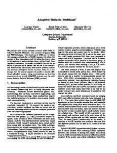
(b) Recovery Cost for Biznet
(c) Retransmission for Biznet Fig. 2.
800
k
(a) Tree Cost for Biznet 6 CPLEX 5 RAERA 4 ST SPT 3 2 1 0 6 8
10
1200
Cost (Tree + Recovery)
20
10
12
70 RAERA 60 ST 50 SPT 40 30 20 10 0 100 200
k
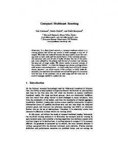
B. Small Real Networks In this subsection, we compare the performance of RAERA, SPT, ST, and the optimal solution generated by CPLEX with different numbers of destination nodes k, where the number of recovery nodes r is selected as 2, and each node is a candidate recovery node in these small networks. Since the RST problem is NP-Hard, CPLEX is able to find the optimal solutions for only smaller instances, and we thus only find an optimal solution for Biznet network. As shown in Fig. 2(a), RAERA generates a solution with the costs that are very close to the optimal solution. The cost of SPT is much higher than others. Compared with SPT, although ST has a smaller tree cost, the distance between the source and a destination is usually higher since the path needs to be deviated from the shortest one in order to aggregate with another path. Therefore, ST tends to incur a higher recovery cost if the recovery nodes are not properly selected, as manifested in Fig. 2(b). In Fig. 2(c), the retransmissions overhead generated by RAERA is still closer to optimal case. In Fig. 2(d), we calculate the average latency of each packet observed by each destination. Since the recovery nodes are closer to the destinations, and the tree depth (i.e., the cost of the longest path in the tree) is restricted by M , which is the cost of the longest path from s to any destination d in SPT, RAERA provides much shorter latency than SPT and ST, and the latency is close to the optimal solution. C. Large Synthetic Networks We also evaluate RAERA, ST, and SPT in larger synthetic networks generated by Inet, where k varies from 100 to 500 , |V | ranges from 4000 to 10000, and r spans from 15 to 55. Compared with smaller networks, the advantage of RAERA is more significant in larger networks. As shown in Fig. 3(a)(b), the total cost increases with k but remains almost the same with |V |. For a larger network, the source and any destination are inclined to be located with more hops away, but there is also a higher chance to find a new path with a lower cost. In average, RAERA limits the total cost by 22% compared to ST and SPT. Fig. 3(e) manifests that all algorithms can effectively lower the recovery cost as r increases, especially RAERA. With a smaller tree and the better selection of recovery nodes, RAERA generates 10% less retransmissions overhead than ST and SPT in Fig. 3(c). Fig. 3(d)(f) present the average latency observed by an individual destination node, and the result shows that RAERA provides 36% shorter latency than ST and SPT.
160
300
400
120
RAERA ST SPT
80 40
500
100
200
k
(d) Latency for Biznet
Simulation results for real networks.
8000 10000
|V|
(a) Cost with different k (|V | = (b) Cost with different |V | (k = 300, 10000, r = 35) r = 35) Retransmission (MBytes)
8
30
1600 RAERA ST SPT 1200
300
400
500
k
(c) Retransmission bytes with dif- (d) Latency with different k (|V | = ferent k (|V | = 10000, r = 35) 10000, r = 35) 1200
Cost (Tree + Recovery)
6
40
Latency (s)
14
CPLEX RAERA ST SPT
50
1100 1000
160
RAERA ST SPT
Latency (s)
18
Cost (Tree + Recovery)
CPLEX 26 RAERA ST 22 SPT
Recovery Cost
Tree Cost
30
900
120
RAERA ST SPT
80 40
800 15
25
35
45
55
15
25
r
35
45
55
r
(e) Cost with different r (|V | = (f) Latency with different r (|V | = 10000, k = 300) 10000, k = 300) Fig. 3.
Simulation results for synthetic networks.
TABLE II. |V | 4000 6000 8000 10000
T HE RUNNING TIME OF RAERA ( SECONDS )
k = 100 0.703 1.4987 2.6102 4.0797
k = 200 1.3694 2.2322 3.3924 4.9029
12 1 2 7
Fig. 4.
k = 300 2.8689 3.902 5.0937 6.6019
k = 400 5.2892 6.9323 7.9065 10.1443
k = 500 9.5575 11.4766 11.9951 13.9863
1 14 11 8 13 1 6 1 8 10 3 5 5 9 1 4 1 1 2 2 6 22 1 1 2 7 3 9 8
The topology for the experimental SDN network.
Table II summarizes the running time of RAERA with different k and network sizes. With a smaller input, such as 4000 nodes and 100 destinations, the running time for RAREA is less than 1 second. As k and |V | increase, the running time grows, but RAERA only spends around 14 seconds in the largest case. Note that according to our online algorithm [26], it is not necessary to re-compute the whole tree when a destination joins or leaves the tree after the tree is initialized with RAERA. It is envisaged that our algorithm is practical to be deployed in SDN networks. D. Implementation To evaluate RAERA in real environments, we implement it in our experimental SDN network including two HP Procurve 3800 and three HP Procurve 5406zl, which are Openflow-enabled switches. We use Floodlight as our Openflow controller to install the traffic routing in SDNFEs. RAERA is running on the top of Floodlight. Because the HP SDN-FEs have not supported local recovery, we implement the recovery nodes in HP ProLiant servers on the top of Click Software Router [34], which is widely adopted in the literature. Since YouTube has not supported
TABLE III.
E VALUATION IN THE EXPERIMENTAL SDN NETWORK
Algorithms RAERA ST SPT
Bandwidth Consumption 13.18 MBytes 16.39 MBytes 17.83 Mbytes
Re-buffering 0.4 s 33.5 s 7.8 s
multicast, a YouTube proxy for multicast is implemented (see the details in [26]). Our SDN testbed includes 14 nodes and 20 links as shown in Fig. 4, and we randomly choose 8 nodes as destinations. We configure each HP switches as multiple SDN-FEs by assigning each slice of the switch as a logical node of the SDN network. Table III summarizes the result on a YouTube video with 136 seconds and 1 MB, where the buffer size of the player in each client is set as 1 second. Table III manifests that the bandwidth consumption of ST and SPT are 24% and 35% more than RAERA, respectively. In addition, we also study the video re-buffering events. We measure the time involved in re-buffering during the whole video playback, and the result shows that RAERA spends less than 1 second, while ST spends 33.5 seconds and SPT spends 7.8 seconds. Therefore, RAERA can effectively improve both the network performance and the user experience. VI.
C ONCLUSION
Current traffic engineering in SDN focuses on only unicast. Compared with forwarding the traffic to each individual destination via unicast, multicast can significantly reduce the network resources consumption. Since many applications (even YouTube) require reliable transmissions, it is envisaged that reliable multicast is important for multicast services in SDN networks. In this paper, therefore, we propose Recover-aware Steiner Tree (RST) for SDN. The RST problem jointly minimizes the tree and recovery costs. We prove that this problem is NP-Hard and inapproximable within k. To solve this problem, we develop an approximation algorithm called Recover Aware Edge Reduction Algorithm (RAERA). Our evaluation shows that RAERA provides lower overall cost, less retransmissions, and lower latency in both real networks and large synthetic networks. In addition, we implement RAERA in a real experiment SDN network, and the results show RST outperforms both SPT and the traditional ST. R EFERENCES [1] “Software-defined networking (SDN): the new norm for networks,” ONF whilte paper. [2] McKeown et al., “OpenFlow: Enabling innovation in campus networks,” SIGCOMM Comput. Commun. Rev., vol. 38, no. 2, pp. 69– 74, Mar. 2008. [3] S. Agarwal, M. Kodialam, and T. Lakshman, “Traffic engineering in software defined networks,” in IEEE INFOCOM’13, pp. 2211–2219. [4] R. Malli, X. Zhang, and C. Qiao, “Benefit of multicasting in alloptical networks,” vol. 3531, pp. 209–220, Nov. 1998. [5] Aggarwal et al., “The effectiveness of intelligent scheduling for multicast video-on-demand,” in ACM MM’09, pp. 421–430. [6] H. Ma, G. K. Shin, and W. Wu, “Best-effort patching for multicast true VoD service,” Multimedia Tools Appl., vol. 26, no. 1, pp. 101– 122, May 2005. [7] Estrin et al., “Protocol independent multicast-sparse mode (PIMSM): Protocol specification,” IETF RFC 2362, May 1998. [8] F. K. Hwang and D. S. Richards, “Steiner tree problems,” Networks, vol. 22, no. 1, pp. 55–89, Oct. 1992.
[9] “Information technology – dynamic adaptive streaming over HTTP (DASH),” ISO/IEC 23009-1, 2014. [10] Floyd et al., “A reliable multicast framework for light-weight sessions and application level framing,” IEEE/ACM Trans. on Networking, vol. 5, no. 6, pp. 784–803, Dec. 1997. [11] B. Whetten and G. Taskale, “An overview of reliable multicast transport protocol II,” IEEE Network, vol. 14, no. 1, pp. 37–47, Jan. 2000. [12] Speakman et al., “PGM reliable transport protocol specification,” IETF RFC 3208, Dec. 2001. [13] “Juniper technical documentation-pgm,” 2014. [Online]. Available: http://www.juniper.net/techpubs/en_US/junos13.2/topics/ reference/configuration-statement/pgm-edit-protocols.html [14] “Cross-platform release notes for cisco IOS release 15.4,” 2014. [Online]. Available: http://www.cisco.com/c/en/us/td/docs/ios/15_ 4m_and_t/release/notes/15_4m_and_t.html [15] G. Robins and A. Zelikovsky, “Improved steiner tree approximation in graphs,” in ACM SODA’00, pp. 770–779. [16] Sushant Jain et al., “B4: Experience with a globally-deployed software defined WAN,” in ACM SIGCOMM’13, pp. 3–14. [17] Qazi et al., “SIMPLE-fying middlebox policy enforcement using SDN,” in ACM SIGCOMM’13, pp. 27–38. [18] J. Mueller, A. Wierz, and T. Magedanz, “Scalable on-demand network management module for software defined telecommunication networks,” in SDN4FNS’13, pp. 1–6. [19] J. Moy, “OSPF version 2,” IETF RFC 2328, Oct. 1998. [20] D.-N. Yang and W. Liao, “On bandwidth-efficient overlay multicast,” IEEE Trans. on Parallel and Distributed Systems, vol. 18, no. 11, pp. 1503–1515, Nov. 2007. [21] E. Aharoni and R. Cohen, “Restricted dynamic steiner trees for scalable multicast in datagram networks,” IEEE/ACM Trans. on Networking, vol. 6, no. 3, pp. 286–297, Jun. 1998. [22] S.-H. Shen and A. Akella, “An information-aware QoE-centric mobile video cache,” in ACM MobiCom’13, pp. 401–412. [23] B. e. a. Adamson, “NACK-oriented reliable multicast (NORM) transport protocol,” IETF RFC 5740, Nov. 2009. [24] B. Fortz and M. Thorup, “Optimizing ospf/is-is weights in a changing world,” Selected Areas in Communications, IEEE Journal on, vol. 20, no. 4, pp. 756–767, Sep. 2006. [25] “IBM ILOG CPLEX,” 2014. [Online]. Available: http://www-01. ibm.com/software/commerce/optimization/cplex-optimizer/ [26] “Reliable multicast routing for software-defined networks.” [Online]. Available: http://www.iis.sinica.edu.tw/~dnyang/SDN/ RAERA.pdf [27] “The implementation for reliable multicast routing for softwaredefined networks.” [Online]. Available: http://www.iis.sinica.edu. tw/~dnyang/SDN/RAERA.tar.gz [28] “The internet topology zoo,” 2014. [Online]. Available: http: //www.topology-zoo.org/dataset.html [29] “EstiNet 8.1 OpenFlow Network Simulator and Emulator,” 2014. [Online]. Available: http://www.estinet.com/ [30] Tangmunarunkit et al., “Network topology generators: Degree-based vs. structural,” in SIGCOMM ’02, pp. 147–159. [31] Balachandran et al., “Developing a predictive model of quality of experience for internet video,” in ACM SIGCOMM’13, pp. 339–350. [32] H. X. Nguyen and M. Roughan, “Rigorous statistical analysis of internet loss measurements,” IEEE/ACM Trans. on Networking, vol. 21, no. 3, pp. 734–745, Jun. 2013. [33] Y. Xu, C. Yu, J. Li, and Y. Liu, “Video telephony for end-consumers: Measurement study of google+, iChat, and skype,” in ACM IMC’12, pp. 371–384. [34] “Click software router,” 2014. [Online]. Available: http://read.cs. ucla.edu/click/click