Remarks on entanglement entropy in string theory - Physical Review

PHYSICAL REVIEW D 97, 066025 (2018)

Remarks on entanglement entropy in string theory Vijay Balasubramanian1,2 and Onkar Parrikar1 1

David Rittenhouse Laboratory, University of Pennsylvania, 209 S.33rd Street, Philadelphia Pennsylvania 19104, USA 2 Theoretische Natuurkunde, Vrije Universiteit Brussel (VUB), and International Solvay Institutes, Pleinlaan 2, B-1050 Brussels, Belgium (Received 31 January 2018; published 28 March 2018) Entanglement entropy for spatial subregions is difficult to define in string theory because of the extended nature of strings. Here we propose a definition for bosonic open strings using the framework of string field theory. The key difference (compared to ordinary quantum field theory) is that the subregion is chosen inside a Cauchy surface in the “space of open string configurations.” We first present a simple calculation of this entanglement entropy in free light-cone string field theory, ignoring subtleties related to the factorization of the Hilbert space. We reproduce the answer expected from an effective field theory point of view, namely a sum over the one-loop entanglement entropies corresponding to all the particle-excitations of the string, and further show that the full string theory regulates ultraviolet divergences in the entanglement entropy. We then revisit the question of factorization of the Hilbert space by analyzing the covariant phase-space associated with a subregion in Witten’s covariant string field theory. We show that the pure gauge (i.e., BRST exact) modes in the string field become dynamical at the entanglement cut. Thus, a proper definition of the entropy must involve an extended Hilbert space, with new stringy edge modes localized at the entanglement cut. DOI: 10.1103/PhysRevD.97.066025

I. INTRODUCTION In this paper, we consider the following question: how does one define entanglement entropy for spatial subregions of the target space in string theory? In ordinary quantum field theory, the entanglement entropy of a subregion inside a spatial slice is defined as the von Neumann entropy of the reduced density matrix on the subregion. However, this definition exploits the inherent locality in the Hilbert space of a “standard” quantum field theory, namely the fact that we can (at least in some lattice approximation) associate independent physical d.o.f. to different points on a given Cauchy surface in spacetime.1; On the other hand, string theory describes fundamentally extended objects, and thus spacetime locality in the sense described above cannot be expected (except in an effective, low-energy sense). This tension between the nonlocality of strings and the requirement of locality for a 1

More precisely, by locality here we mean that the total Hilbert space can be expressed as a tensor product HΣ ¼⊗x∈Σ Hx of Hilbert spaces associated with individual points x in a Cauchy surface Σ. Published by the American Physical Society under the terms of the Creative Commons Attribution 4.0 International license. Further distribution of this work must maintain attribution to the author(s) and the published article’s title, journal citation, and DOI. Funded by SCOAP3.

2470-0010=2018=97(6)=066025(15)

conventional definition of entanglement entropy for spatial subregions is the fundamental obstacle which forbids a straightforward definition. Previous attempts at computing entanglement entropy in string theory have focussed on using the replica trick as a prescription [1–6], and the resulting quantity is often referred to as the conical entropy. This is not entirely satisfactory because it involves studying the perturbative string partition function on an off-shell background involving a conical singularity at the entanglement cut. Nevertheless, these calculations have yielded interesting insights; for instance, [1] argued in the context of black hole entropy in closed string theory that the sphere diagram straddling the horizon gives the “classical” Bekenstein-Hawking entropy. The authors further interpreted this diagram as counting the states of open strings ending on the horizon, thus leading to a microscopic picture for the classical black hole entropy in terms of open strings ending on the horizon. This picture was recently explored further in the context of the string theory dual to large N 2d Yang-Mills in [7]. In a separate recent development, [4–6] computed the one-loop entanglement entropy across a Rindler horizon and argued for the UV finiteness of the entropy in closed superstring theory:

066025-1

SEE ¼ s

A⊥ þ ; α04

ð1Þ

Published by the American Physical Society

PHYS. REV. D 97, 066025 (2018)

VIJAY BALASUBRAMANIAN and ONKAR PARRIKAR where s is a dimensionless, Oð1Þ constant. However, it would be nice to have an independent definition of entanglement entropy in string theory not relying on the replica trick. Before moving to strings, let us briefly revisit the setup for studying entanglement in conventional theories of point particles. In this case, it is convenient to use the quantum field theory description instead of the “firstquantized” worldline description. That is, instead of using the worldline variables (the position and intrinsic metric Xμ ðτÞ; gττ ðτÞ), one switches over the to the quantum field operator ΦðXμ Þ; which is an operator-valued function on the target spacetime M. One then picks a Cauchy surface Σ in M, which for simplicity we can choose to be X0 ¼ 0. Since operators separated along Σ commute, one can think of the operators at each point on Σ as independent. In studying the spatial entanglement structure of a state, one then partitions Σ into two (or more) regions, and computes the reduced density matrix on a given subregion, which corresponds to tracing out all the operators outside the region of interest. Now we wish to follow the same line of thought for string theory. For simplicity, we will consider bosonic open string theory on Minkowski spacetime M ¼ R1;25 , but we expect that our setup can straightforwardly be generalized to superstrings, and even to closed strings at some level. Following the logic outlined above, we wish to pass from the world sheet description to a “field theory” description. Naturally, since string theory describes strings as opposed to point particles, the corresponding string field operator Φ is an operator-valued function not on the target spacetime M, but on “the space of all open strings in spacetime” Φ½Xμ ðσÞ; where as mentioned above, Xμ ∶½0; π → M is an open string configuration in M. We will call this “space of all open strings in spacetime” Mopen . (If we were considering closed string theory, then Mclosed would be the loop space of M.) More precisely, the string fields also depend on ghost-configurations, but since we will not be interested in entanglement cuts along anticommuting directions, we suppress them for now. We can be a little more explicit about Mopen by modeexpanding the open-string configuration Xμ ðσÞ ¼ Xμ0 þ

∞ X

2Xμn cosðnσÞ;

ð2Þ

n¼1

and treating the coefficients Xμn as coordinates on Mopen . The next step is to pick a Cauchy surface S inside Mopen . We can choose S, for instance, to be the surface consisting of open strings with the time component of the center of mass

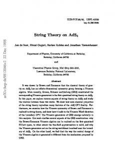
FIG. 1. (Left) From a spacetime point of view, we’re interested in the d.o.f. inside a subregion R of the Cauchy Surface S. However, in string theory we can have strings which either lie in R (blue), or straddle the cut ∂R (violet), or lie outside R (red). (Right) In string field theory, we get around this issue by considering a subregion R inside the space of open string configurations. One natural choice of the subregion is the trivial extension of R along the stringy directions X μn>0 ; the open string configurations from the left panel are displayed as points.

coordinate X00 fixed, or somewhat more generally tμ Xμ0 fixed, where tμ is a timelike vector.2 The phase space of the theory can then be established by constructing a symplectic form on S [9]. From standard reasoning, string-fields at different points on S commute ½Φ½Xμ ðσÞ; Φ½Y μ ðσÞ ¼ 0;

Xμ ;

Y μ ∈ S:

ð3Þ

Equivalently, we can think of string field operators at different points on S as being independent d.o.f. In order to study the entanglement properties of the vacuum in this theory, we can partition the surface S into subregions. Note that this is very different from the situation in ordinary field theory—here we are required to partition not a Cauchy surface Σ in the target spacetime M, but instead an infinite-dimensional surface S in the space of open string configurations Mopen . A partition of Σ of course does not extend to a partition of S in a unique way—indeed given a subregion R ⊂ Σ, there are many ways to extend this to a subregion R ⊂ S, and the results of our computations will depend on the choice of extension. One natural choice from the spacetime point of view is to extend the subregion as follows (see Fig. 1): R ¼ fXμ ðσÞ ∈ SjX μ0 ∈ Rg:

ð4Þ

R consists of all strings with their center-of-mass inside the spacetime region R; this does not mean that the entire string is contained in R. In particular, R includes strings which straddle the entanglement cut ∂R from a spacetime point of view. (Of course, another interesting possibility is to choose 2

Another natural choice in Witten’s cubic string field theory [8] is to consider the space of all open strings with the midpoint time coordinate fixed, i.e., tμ X μ ðπ=2Þ ¼ 0. More on this in later sections.

066025-2

REMARKS ON ENTANGLEMENT ENTROPY IN STRING THEORY R such that the entire string is contained inside R, but we will not attempt this here; we will briefly return to this point in the Discussion.) In any case, once we choose the subregion R, the reduced density matrix over R, and subsequently the entanglement entropy, can be defined and computed in the standard way, much like in conventional quantum field theory. So string field theory provides a potentially feasible and welldefined way to study the entanglement structure of the vacuum in string theory. In this paper, we wish to take the first steps in this direction. The rest of the paper is organized as follows. In Sec. II, we will compute the entanglement entropy (following the definition explained above) in free string field theory (gs → 0) in the light-cone gauge. In this computation we will ignore subtleties associated with the factorization of the Hilbert space. This will serve mainly as a sanity check on our proposed definition, as we will show that the entanglement entropy agrees with the expected answer from a spacetime effective field theory point of view. Then, in Sec. III, we will recall that string field theory has a gauge symmetry which interferes with factorization of the Hilbert space on S ⊂ Mopen . We will address this issue by analyzing the covariant phase space corresponding to a subregion in covariant string field theory (again in the free limit), following the framework of Donnelly and Friedel [10]. We will show that BRST exact modes in string field theory become dynamical at the entanglement cut, much like in conventional gauge field theories where edge modes appear in the computation of entanglement entropy. II. ENTANGLEMENT ENTROPY IN LIGHT-CONE GAUGE In this section, we will consider free bsosonic, open string field theory (OSFT) in D ¼ 26 spacetime dimensions. We will use the light-cone gauge for OSFT following [11–15] in our analysis; see also [16] which studies covariant string field theory in Rindler space.3 We will consider a half-space R in spacetime, and the corresponding extension R (as in equation (4) to the space of all open strings. The computation in this section is a simplified version of the full story, because it ignores the lack of factorization of the OSFT Hilbert space, an issue that we will address in the next section. We choose light-cone coordinates: X ¼ X0  XD−1

ð5Þ

in terms of which the metric of Minkowski spacetime is ⃗ i dX ⃗ i: ds2 ¼ −dXþ dX− þ dX

ð6Þ

PHYS. REV. D 97, 066025 (2018)

In the light cone gauge, we fix Xþ to be σ-independent: Xþ ðσÞ ¼ xþ

ð7Þ

X− ðσÞ ¼ x−0 þ   

ð8Þ

⃗ i ðσÞ ¼ xi0 þ X

∞ X l¼1

2xil cosðlσÞ:

ð9Þ

where the    denote oscillator modes along the − direction, which get fixed in terms of the remaining modes by the constraint that the world sheet stress tensor vanishes. ⃗ i ðσÞ, with an The string field takes the form Φ½xþ ; x−0 ; X equation of motion  Z π  ∂2Φ δ2 ⃗ 2 ðσÞ Φ: ð10Þ −2 þ − ¼ þ ∂σ X dσ − 2 ⃗ ðσÞ ∂x ∂x0 δX 0 where we have set α0 ¼ 1. We can write equivalently this in terms of the following action  Z Z 1 ∂2 þ − ⃗ S0 ¼ dx dx0 ½dXðσÞ 2Φ þ − Φ 2 ∂x ∂x0   Z π  2 δ 2 ⃗ þ ∂ σ X ðσÞ Φ : þΦ dσ − 2 ð11Þ ⃗ ðσÞ δX 0 It seems natural to quantize this system on the xþ ¼ 0 surface, i.e. by treating xþ as time. However, light-front quantization is fairly subtle, because if we want to regard xþ as time, then the Lagrangian is first order in ∂ þ Φ [17]. Consequently, it is not consistent to think of Φ and Π ∼ ∂ − Φ as independent operators. In other words, light-front quantization amounts to quantizing a constrained system, and one has to use Dirac brackets. In order to avoid these complications, we will follow a different approach and define new coordinates x− → x− ;

1 xþ → xþ þ εx− 2

ð12Þ

In terms of these coordinates, the action becomes    Z Z 1 ∂2 ∂2 ⃗ Φ 2 þ − þε þ þ Φ S0 ¼ dxþ dx−0 ½dXðσÞ 2 ∂x ∂x0 ∂x ∂x   Z π  2 δ þΦ dσ − 2 þ ∂ σ X⃗ 2 ðσÞ Φ : ð13Þ δX⃗ ðσÞ 0 Now the action is quadratic in ∂ þ Φ (after integration by parts), and we can quantize this system canonically. The conjugate momentum is Π ¼ ∂ − Φ þ ε∂ þ Φ:

ð14Þ

3

The approach in [16] is similar in spirit to our calculations in Sec. II. We thank Thomas Mertens for bringing [16] to our attention, after the first version of our paper was uploaded to the arXiv.

We can expand the string field operator in terms of solutions to the equation of motion derived from the above action. This gives

066025-3

PHYS. REV. D 97, 066025 (2018)

VIJAY BALASUBRAMANIAN and ONKAR PARRIKAR ⃗ Φ½xþ ; x−0 ; XðσÞ ¼

Z

dD−2 ⃗p ð2πÞD−2

 ∞ X Y dpþ 1 −iðpþ x−0 þp− xþ − ⃗p·⃗x0 Þ þ pffiffiffiffiffiffiffiffiffiffiffiffiffiffiffiffiffiffiffiffiffiffiffiffiffiffi a e f ð⃗ x Þ þ H:c: ; p ; ⃗p;f⃗nl g n⃗ l l 2ðpþ þ εp− Þ f⃗n g −∞ 2π l¼1

Z

∞

l

where in the oscillator directions we have the simpleharmonic oscillator wave functions

f n⃗ l ð⃗xl Þ ¼

D −2 Y i¼1

i 2

Hnil ðxil Þe−lðxl Þ ;

⃗ ⃗ GΦ;Φ ð0; x−0 ; Xj0; y−0 ; YÞ Z Z pffi − − ∞ dpþ X 1 dD−2 ⃗p þ eip εðy0 −x0 Þ−i ⃗p·ð⃗y0 −⃗x0 Þ ¼ D−2 ð2πÞ −∞ 2π f⃗n g 2ω l

ð16Þ ×

∞ Y l¼1

and there is a dispersion relation p− þ

pþ ¼ ε

 þ2 ⃗p2 þ p þ 2 ε

P∞

l¼1

l

i¼1

ε

nil

1=2 :

ð17Þ

l

¼ ð2πÞD−2 δD−2 ð ⃗p − ⃗p0 Þ2πδðpþ − pþ0 Þδf⃗nl g;f⃗n0l g : ð18Þ The normalization for the oscillators is chosen such that

ω¼

⃗ y−0 ÞδðXðσÞ

∞ D−2 X X l nil pþ2 þ ⃗p2 þ

⃗ 0 ÞÞ: − Yðσ

ð23Þ

⃗ ⃗ ¼ − i δðx−0 − y−0 ÞδðXðσÞ ⃗ ⃗ 0 ÞÞ; GΦ;Π ð0; x−0 ; Xj0; y−0 ; YÞ − Yðσ 2 ð24Þ ⃗ ⃗ GΠ;Π ð0; x−0 ; Xj0; y−0 ; YÞ Z Z pffi − − ∞ dpþ X εω dD−2 ⃗p þ eip εðy0 −x0 Þ−i ⃗p·ð⃗y0 −⃗x0 Þ ¼− D−2 ð2πÞ −∞ 2π f⃗n g 2 ×

ð19Þ

ð20Þ

Of course, in bosonic string theory this vacuum is unstable as indicated by the presence of a tachyon in the spectrum, but we will continue to work with this state here. In order to compute the entanglement entropy, we will need the various equal-time two-point functions of the string field Φ and its momentum. The Φ − Φ correlator is ⃗ ⃗ GΦ;Φ ð0; x−0 ; Xj0; y−0 ; YÞ ⃗ ⃗ 0 ÞÞj0i y−0 ; Yðσ ¼ h0jΦð0; x−0 ; XðσÞÞΦð0;

:

i¼1

l

The vacuum j0i of string field theory satisfies apþ ; ⃗p;f⃗nl g j0i ¼ 0:

!1=2

Similarly, the other two-point functions are given by

⃗ ⃗ 0 ÞÞ Πðxþ ; y−0 ; Yðσ ½Φðxþ ; x−0 ; XðσÞÞ; −

ð22Þ

l¼1

½apþ ; ⃗p;f⃗nl g ; a†pþ0 ; ⃗p0 ;f⃗n0 g 

¼

f n⃗ l ð⃗xl Þf n⃗ l ð⃗yl Þ

where we have defined PD−2

Further, a†pþ ; ⃗p;f⃗nl g and apþ ; ⃗p;f⃗nl g are operators which create and annihilate strings with the specified mode occupation numbers.4 They satisfy the commutation relations

−iδðx−0

ð15Þ

∞ Y l¼1

f n⃗ l ð⃗xl Þf n⃗ l ð⃗yl Þ:

ð25Þ

In order to compute the entanglement entropy, we will use the algebraic definition in terms of correlation functions [18,19]. Let us consider the half-space x− > 0 on the spacetime Cauchy surface xþ ¼ 0.5 As discussed in the introduction, we wish to extend this to a subregion R in the space of open strings. This extension is not unique, but we use the simplest one, − ⃗ R ¼ fx−0 ; XðσÞjx 0 > 0g;

ð26Þ

which is the analog of Fig. 1 for a half-space. The basic idea in the algebraic method [18,19] is that for bosonic Gaussian systems, the reduced density matrix is the exponential of a bilocal operator of the form:

ð21Þ ρ∼e

P

−

ij

ðAij Φi Φj þBij Φi Πj þCij Πi Πj Þ

;

ð27Þ

is given by 5

4

Not to be confused with the usual first-quantized string oscillators αμn which create modes on a given string.

Our general conclusions do not depend on this particular choice of half-space (i.e., we could have equally well picked other regions), although of course the specific expression will do so.

066025-4

REMARKS ON ENTANGLEMENT ENTROPY IN STRING THEORY where the indices i; j… denote spatial coordinates restricted to the region R for ordinary quantum fields on a lattice. In the continuum the sums on indices become integrals, and in the present case they become integrals on the string coordinates restricted to R. By definition, the reduced density matrix should reproduce the correct correlation functions for operators inside R, so the matrices A, B and C can be recovered from the knowledge of two-point functions of Φ and Π restricted to R. We will not go through the details of this calculation here, but we merely state the result. Let us define the matrix − ⃗ ⃗ C2 ðx−0 ; XðσÞjy 0 ; YðσÞÞ Z Z ∞ − − ⃗ − ⃗ ⃗ ¼− dz0 ½dZðσÞG Φ;Φ ðx0 ; Xjz0 ; ZÞ 0

⃗ −0 ; YÞ ⃗ × GΠ;Π ðz−0 ; Zjy

ð28Þ

⃗ integral is restricted to the subregion where the ðz−0 ; ZðσÞÞ R. In terms of the matrix C, the entanglement entropy is formally given by6 SEE ðRÞ ¼ TrððC þ 1=2Þ lnðC þ 1=2Þ − ðC − 1=2Þ lnðC − 1=2ÞÞ:

ð29Þ

Since we know the two-point functions of the string fields, we can easily compute C2 : ⃗ −0 ; YÞ ⃗ ¼ C2 ðx−0 ; Xjy

X Γf⃗nl g ðx−0 ; x⃗ 0 ; y−0 ; y⃗ 0 Þ f⃗nl g

×

∞ Y l¼1

f n⃗ l ð⃗xl Þf n⃗ l ð⃗yl Þ;

ð30Þ

where pffiffiffi Z D−2 Z ∞ þ i ε d p⃗ ip·ð dp ⃗ ⃗x0 − ⃗y0 Þ e Γf ⃗nl g ¼ D−2 4 ð2πÞ −∞ 2π Z ∞ þ −ipffiεðpþ x− −qþ y− Þ qþ2 þ þp⃗ 2 þ μ2 1=2 0 0 dq e f ⃗nl g ; × þ þ p −q pþ2 þ p⃗ 2 þ μ2f ⃗nl g −∞ 2π ð31Þ μ2⃗p;f⃗nl g ¼

∞ D−2 X X l nil : l¼1

ð32Þ

It is clear from Eq. (30) that the matrix C2 is blockdiagonal in terms of the oscillator excitations of the open string, namely j0i; αi−1 j0i; αi−1 αj−1 j0i;   ; namely Eq. (30) has single sum over n⃗ l. This is essentially a direct consequence of the fact that the subregion R is a direct product of the spacetime subregion R and the oscillator directions Xμn>0 . Therefore, the entanglement entropy takes the form X SEE ¼ SEE ðμ2f⃗nl g Þ; ð33Þ f⃗nl g

where SEE ðμ2f⃗nl g Þ is the entanglement entropy for a scalar of mass μf⃗nl g , as should be clear from the above interpretation of the structure of Γ. In other words, every excitation in the list j0i; αi−1 j0i; αi−1 αj−1 j0i;    adds one scalar degree of freedom worth of entropy, with the appropriate mass. This result makes sense physically, because in the free limit, the various oscillator modes of the string are entirely decoupled, and should contribute independently to the entanglement. Equivalently, we may group the various oscillator excitations in terms of representations of the Poincar´e group according to mass and spin, and as a result, equation (33) can be thought of as summing over the entanglement entropies corresponding to the various fields in the open-string spectrum, i.e., the tachyon j0i, the photon αi−1 j0i, the massive, symmetric-traceless spin-2 field αi−1 αj−1 j0i ⊕ αi−2 j0i etc., where the tachyon contributes one scalar degree of freedom, the photon contributes 24 d.o.f., the spin-2 field contributes 324 d.o.f. etc. Note that since we are computing the entanglement entropy algebraically, we do not encounter the additional “contact terms” which appear in the conical entropy [4,20]; we will come back to this in the next section. In order to obtain an explicit expression for SEE we would ordinarily have to diagonalize the matrix Γf⃗nl g . However, this is unnecessary in the present case; the halfspace entropy of a massive scalar field in d-dimensions is already well known (see [4], for instance) Z ∞ 1 ds 1 2 SEE ðm2 Þ ¼ A⊥ e−sm ; ð34Þ d=2−1 2 6 2s ð4πsÞ ε where A⊥ is the area of the entanglement cut, and ε is an ultraviolet cutoff. This integral is UV divergent, and takes the form  −m2 ε2 X n−1 1 A⊥ e ð−1Þk ðn − k − 1Þ!ðmεÞ2k 12 ð4πÞn n! ε2n k¼0  n − ð−1Þ ð2lnðmεÞ þ γÞ þ OðmεÞ ð35Þ

i¼1

The reader can check that Γ is identical to the corresponding matrix −Gϕϕ · Gππ for a real scalar field of mass μ2 (restricted to the half space).

PHYS. REV. D 97, 066025 (2018)

SEE ðm2 Þ ¼

6

In order to make these manipulations concrete (i.e., to make sense of the infinite-dimensional integrals), we can discretize the string and pick a lattice in the target space.

where n ¼ d2 − 1. However, string theory softens these divergences to a great extent. In order to see this, we first

066025-5

PHYS. REV. D 97, 066025 (2018)

VIJAY BALASUBRAMANIAN and ONKAR PARRIKAR perform the sum in Eq. (33) before carrying out the s-integral (restoring α0 ): SEE ¼

A⊥ 6

Z

∞

ε2

∞ X ðN−1Þ ds 1 degN e−s α0 ; d=2−1 2s ð4πsÞ N¼0

ð36Þ

ηði=tÞ ¼ t1=2 ηðitÞ; 2

where degN is the number of states at mass m ¼ P 0 Defining q ¼ e−s=α and writing N ¼ μ;n nN μ;n , we can perform the sum in the standard way [21]: ∞ X

ðN−1Þ α0

−s

degN e

¼

q−1

24 Y ∞  Y μ¼1 n¼1

N¼0

¼

∞ 1 Y

∞ X

N−1 α0 .

 qnN μ;n

N μ;n ¼0

24

¼ ηðis=2πα0 Þ−24 ;

ð37Þ

where the Dedekind eta function is defined as ηðτÞ ¼ q1=24

∞ Y ð1 − qn Þ;

q ¼ e2πiτ :

Z

1 A⊥ 2 6 ð8π α0 Þd=2−1

Z

∞

ε20

1=ε20 1

n¼1

SEE ¼

1 A⊥ ¼ 6 ð8π 2 α0 Þd=2−1

dt 1 ηðitÞ−24 ; 2t td=2−1

ε20 ¼

ε2 : 2πα0 ð39Þ

Note that the entropy is proportional to the area of the entangling surface. As usual, this means that the entropy comes from the short-distance entanglement across the cut. d−2 Crucially, the prefactor is proportional to α0− 2 , as opposed to the corresponding power of the UV cutoff (see below for further justification) which is typical of standard quantum field theories. This indicates that in string theory, the entanglement comes from string-scale correlations across the cut, and is another manifestation of the UV finiteness of string theory. Let us now analyze the divergences in the entanglement entropy. As is familiar from standard considerations in string theory, there are two types of divergences in the above integral: t → 0 (UV divergence) and t → ∞ (IR divergence). We can analyze the t → ∞ divergence by expanding the eta function: ηðitÞ−24 ¼ e2πt þ 24 þ Oðe−2πt Þ

ð40Þ

where the various terms in this expansion should be thought of, similar to the left hand side of equation (37), as corresponding to on-shell states of different m2 . The first term (which is due to the tachyon) gives a divergence in the t → ∞ limit, but this is unphysical anyway because the

Z 0

1=ε20

ds ηðisÞ−24 : 2s

ð42Þ

Now we again expand in the large s limit using ηðisÞ−24 ¼ e2πs þ 24 þ Oðe−2πs Þ. Once again we see that we encounter a tachyonic divergence in this “closed-string” channel (which would not appear in the superstring, but can be regulated here using analytic continuation). In addition we have a logarithmic divergence from the zero modes which is of the form

ð38Þ

So we have the final result

ð41Þ

to rewrite the entropy as SEE

1 ð1 − qn Þ n¼1

q

tachyon will be projected out in the superstring. The remaining terms do not give any divergences as t → ∞. Now consider the t → 0 (UV) limit. Here, we can switch to s ¼ 1=t and use the property

  ds 2πα0 ∼ ln : s ε2

ð43Þ

The massive modes do not give any divergences in this limit. This story entirely parallels the standard divergence structure of the one-loop (cylinder) diagram in open string theory. In that case, the above divergence coming from zero modes in the closed-string channel is cancelled out in the full unoriented, open plus closed string theory, provided we choose the right gauge group (SOð32Þ in the superstring). We expect a similar cancellation to occur in the case of entanglement entropy, but this calculation will require a careful analysis of the entropy for closed strings. In this section, we have demonstrated that in the free limit (gs → 0), the entanglement entropy computed using open string field theory is consistent with expectations from the effective field theory of the open-string excitations. Namely, the answer we obtained was essentially the halfspace entanglement entropy in a theory with an infinite number of free particles with the required masses and spins (minus degrees freedom removed by gauge symmetry). However, for finite gs and certainly in closed string theory, we expect this not to be generically true and the effective field theory approach should break down.7 For this reason, it is important to have an intrinsically stringy definition of 7

For instance, the one-loop diagram in closed string theory does not have UV divergences because of the restricted region of integration in the modular parameter τ of the torus, while a naive sum over the one-loop contributions from the particle excitations is UV divergent [22]. Similarly, we expect that in computing entanglement entropy for closed strings, one must carefully account for the correct region of integration for the modular parameter, something which is nontrivial in closed string field theory [23–25].

066025-6

PHYS. REV. D 97, 066025 (2018)

REMARKS ON ENTANGLEMENT ENTROPY IN STRING THEORY the entanglement entropy, such as the one we have advocated using string field theory. III. COVARIANT PHASE SPACE FOR SUBREGIONS In the previous section, we neglected the gauge symmetry of open string field theory and the associated failure of factorization of the Hilbert space. In this section we will address this issue from the point of view of Witten’s covariant open string field theory [8,9] (see the Appendix for a lightning review). We will follow the method outlined by Donnelly and Freidel in [10] to analyze the phase space of string field theory on a subregion of the space of open string configurations. This will lead us to an extended Hilbert space picture, with stringy edge modes localized at the entanglement cut.

the space of initial conditions. In quantum field theory, since these initial conditions are functions of a Cauchy surface Σ in spacetime, the symplectic 2-form can be written as an integral of a density on Σ: Z ω¼ J; with d⋆J ¼ 0: ð47Þ Σ

The density J must be conserved, because conservation ensures that the symplectic structure does not depend on the choice of Σ. Now we wish to construct such a symplectic 2-form for OSFT, which in the present case will be localized on a Cauchy surface S ⊂ Mopen . For this purpose, let us first pick a Cauchy surface Σ in the target spacetime, and let θ be defined as the following function of the string center of mass:  θðΣÞ ¼

A. Symplectic structure Witten’s covariant open string field theory is constructed in terms of the string field A½Xμ ðσÞ; b ðσÞ; c ðσÞ which is an element of the one-string Hilbert space which we will call B here. Here Xμ are coordinates in target space and b and c are auxiliary ghost fields. It is possible to define a non-commutative star product R on this space, together with the notion of “integration” , in terms of which the action takes the Chern-Simons form  Z  1 2 S¼ 2 A  QA þ A  A  A ; ð44Þ 3 gs where Q is the BRST operator (Appendix contains a brief review of the requisite background material, together with explicit expressions for , Q etc.). The equation of motion is given by QA þ A  A ¼ 0:

ð45Þ

Further, this action has the gauge symmetry δA ¼ Qε þ A  ε − ε  A:

1 Xμ0 > Σ

0 Xμ0 < Σ;

ð48Þ

with the notation Xμ0 > Σ (Xμ0 < Σ) meaning that the point Xμ0 lies to the future (past) of Σ. Further, let us define δ to be the exterior derivative on the phase space P, namely the space of solutions to the equation of motion QA þ A  A ¼ 0. Then, for instance, δA is a 1-form on the phase space, satisfying the linearized equation of motion around A. The symplectic 2-form on P is then given by Z ω ¼ δA  ½Q; θðΣÞδA; ð49Þ where we have left the wedge product between differential forms on P implicit. Firstly, note that ω is a 2-form on P. The BRST charge Q has derivatives with respect to the string coordinates, and so the commutator ½Q; θðΣÞ is proportional to a delta function for the center of mass lying on Σ; in other words the symplectic 2-form is localized on the Cauchy surface S ⊂ Mopen . Finally, ω is independent of the choice of Σ because given two surfaces Σ1 and Σ2 : Z ωΣ1 − ωΣ2 ¼ QðδA  fðΣ1 ; Σ2 ÞδAÞ ¼ 0; ð50Þ

ð46Þ

Linearized about A ¼ 0, Eqs. (45) and (46) imply the statement that physical (on-shell) states are in the BRST cohomology. We will focus on this free limit in our discussion below. The important object for our discussion is the symplectic 2-form for OSFT constructed by Witten in [9] using the covariant phase space approach (see also [26]). In this formalism, we identify the space of solutions of the equations of motion as the phase space P; this is because the space of solutions is in one-to-one correspondence with

where the right-hand side vanishes because the function RfðΣ1 ; Σ2 Þ ¼ θðΣ1 Þ − θðΣ2 Þ vanishes at infinity, and so Qð  Þ ¼ 0. In [9] Witten used the string midpoint (instead of the center of mass) in the above construction. The choice of the midpoint is of course very natural in Witten’s OSFT, but on the other hand from the point of view of the constituent fields, it seems more natural to use the center of mass of the string. We expect that at least in the free theory (gs → 0) which is the case we are focussing on, both the choices should be equivalent. At any rate, the symplectic form

066025-7

PHYS. REV. D 97, 066025 (2018)

VIJAY BALASUBRAMANIAN and ONKAR PARRIKAR Z ω¼

δ  AD0 δA ¼ hδAjD0 δAi;

ð51Þ

where D0 ¼ ½Q; θðΣÞ is defined in terms of the center of mass, has all the necessary properties, as explained above.8 For simplicity, let us take the surface Σ to be at tμ Xμ0 ¼ 0, where we can take tμ ¼ ð1; 0; …; 0Þ or a more general timelike vector. Using Eq. (A3), we can compute the commutator D0 : i D0 ¼ − c0 ðt · α0 δðtμ Xμ0 Þ þ δðtμ Xμ0 Þtμ αμ0 Þ 2 X − iδðtμ Xμ0 Þ c−n tμ αμn :

ð52Þ

careful with such “total derivative” terms when we deal with the symplectic structure associated with subregions. Indeed, when we consider the phase space for subregions, this gives rise to nontrivial d.o.f. at the boundary of the subregions. B. Symplectic structure for subregions Let us now consider the symplectic structure corresponding to a subregion R ⊂ Σ. For simplicity, we can take R to be a half-space X1 > 0. However, recall that by a subregion here we should mean a subregion in the Cauchy surface S inside the space of open strings Mopen . As before, we pick the simplest extension9:

n≠0

To check for gauge invariance of the symplectic form at the level of the string fields, we must verify that it vanishes when evaluated on a pure gauge mode ωðQε; ΨÞ ¼ 0;

ð53Þ

for any physical mode Ψ satisfying QΨ ¼ 0. This is the physical requirement that pure gauge modes are not dynamical. By explicit calculation, we obtain Z ωðQε; ΨÞ ¼ ðQε  D0 Ψ − Ψ  D0 QεÞ Z ¼ Qðε  D0 Ψ − Ψ  D0 εÞ ¼ 0:

ð54Þ

R In the last line, we have used the fact that Qχ ¼ 0, which is true as long as χ vanishes at infinity. We have therefore demonstrated that the pure gauge modes in the string field do not have any symplectic structure associated with them, and that ω simply pulls-back to the moduli space of string fields modulo gauge transformations. This is generically true in the situation where Σ has no boundaries, or the string field variations vanish at infinity. However, one has to be 8 To see that this agrees with the standard symplectic structure for component fields, let us consider the photon field which appears at level one. Using (A20), we can compute the symplectic 2-form:

ω¼

1 2

Z

R ¼ fXμ ðσÞ ∈ SjX10 > 0g: The symplectic two-form restricted to the region R is then given by Z ωR ¼ δA  θðRÞD0 δA ¼ hδAjθðRÞD0 δAi; ð55Þ where by θðRÞ we mean  1 θðRÞ ¼ 0

which upon using the equations of motion 2δf ¼ ∂ μ δAμ gives the standard symplectic form for the U(1) gauge field, up to boundary terms (at spatial infinity):

A ¼ a þ Qε:

0

μ

d xδðx ÞδA δF0μ :

ð57Þ

The one-form δA then becomes δA ¼ δa þ Qδε;

ð58Þ

where we could think of δε as the linearized Maurer-Cartan form for the gauge group. Substituting this in Eq. (55), we find Z ωR ¼ δa  θðRÞD0 δa Z þ ðδa  D1 D0 δε − δε  D1 D0 δa − δε  D1 D0 QδεÞ:

The first term above is the standard symplectic form pulled back on to the moduli-space of string fields (modulo gauge transformations), and has support over the entire region R. 9

d

ð56Þ

ð59Þ

− 2δA0 δf þ 2δfδA0 Þ;

Z

Xμ ðσÞ ∉ R:

We now revisit the issue of gauge-invariance. In order to be more systematic, let us choose coordinates A ¼ ða; εÞ on the space of string fields satisfying the equations of motion, where a corresponds to the moduli-space of string fields modulo gauge transformations, and ε denotes the pure gauge directions:

dd xδðx0 ÞðδAμ ð∂ 0 δAμ Þ − ð∂ 0 δAμ ÞδAμ

1 ω¼ 2

Xμ ðσÞ ∈ R

We are suppressing the dependence on ghosts here because the subregion includes the entire space of ghost configurations, i.e. we do not partition along the anticommuting directions.

066025-8

REMARKS ON ENTANGLEMENT ENTROPY IN STRING THEORY The remaining terms indicate that the pure gauge modes do not entirely decouple in the presence of the entanglement cut. Note that the operator D1 ¼ ½Q; θðRÞ is given by i D1 ¼ − c0 ðrμ αμ0 δðrμ Xμ0 Þ þ δðrμ Xμ0 Þrμ αμ0 Þ 2X − i δðrμ Xμ0 Þc−n rμ αμn ;

ð60Þ

because ωR depends only on δε and not on ε, where the former is invariant under this left-action because α is a constant with respect to the string phase space coordinates ða; εÞ. We can easily write down the generators of these boundary symmetries—recall from Hamiltonian mechanics (written in terms of symplectic geometry) that this amounts to constructing charges J½α such that

n≠0

I V α ωR ¼ δJ½α;

μ

where r ¼ ð0; 1; 0; …; 0Þ is the spacelike normal vector to the boundary ∂R. The delta functions in D1 clearly imply that these gauge-dependent terms are localized on the boundary of the subregion. In other words, the pure gauge modes become dynamical at the entanglement cut, giving rise to stringy edge modes. The fact that the symplectic 2-form for a subregion is not gauge-invariant is a standard feature of gauge theories [10,27]. It indicates that the Hilbert space does not factorize between subregions. Our discussion above shows that a similar situation arises in string field theory, and therefore care must be taken in defining the entropy of a subregion. The power of string field theory is that we need not revisit string quantization again in the presence of the entanglement cut to deduce these edge modes—we can simply use gauge invariance in string field theory. One approach to deal with nonfactorization of Hilbert spaces in gauge theories is the extended Hilbert space formalism [10,27–32]. In this formalism, one embeds the physical Hilbert space as a subspace inside an extended Hilbert space: Hext ¼ HRb ⊗ Hedge ⊗ Hedge ⊗ HRb :

ð61Þ

where HRb and HRb are the Hilbert spaces in the bulk of the region R and its complement. The extended Hilbert space includes two copies of edge modes (corresponding ¯ and involves many nonphysical states, but to ∂R and ∂ R) has the virtue that it factorizes naturally. Once the physical state of interest can be identified inside the extended Hilbert space, one can trace out the complement and define entanglement entropy in the standard way. In order to proceed, we need to understand how to construct Hedge . To that end, it is useful to characterize the edge modes by making explicit the global symmetries acting on them. Note, for instance, that the symplectic form is invariant under the “left-action”10 δL a ¼ 0;

δL ε ¼ −α;

ð62Þ

One can also define a “right-action”

10

δR a ¼ −Qβ;

δR ε ¼ β

which is a mere redundancy of our parametrization (57). The notation left and right is ambiguous in free string field theory, but becomes meaningful in the full nonlinear version.

PHYS. REV. D 97, 066025 (2018)

ð63Þ

where I X is the interior product on differential forms on P (given some vector field X on P). For instance, I X ω ¼ ωðX; ·Þ. The vector field V α above generates the left action on phase space, and therefore satisfies I V α δε ¼ −α. Now, a simple computation shows that Z I V α ωR ¼ ðδa  D1 D0 α þ α  D1 D0 δa þ α  D1 D0 Qδε − δε  D1 D0 QαÞ;

ð64Þ

and so we can read off the currents from here Z J½α ¼ ða  D1 D0 α þ α  D1 D0 a þ α  D1 D0 Qε − ε  D1 D0 QαÞ:

ð65Þ

A further simple calculation shows that these currents satisfy the following current algebra: Z fJ½α;J½βgP:B ¼ ðα  D1 D0 Qβ − β  D1 D0 QαÞ: ð66Þ Therefore, the Hilbert space of the edge modes Hedge should furnish a representation of this current algebra (in the gs → 0 limit). The next question is how to identify physical states (let us say the vacuum) inside the extended Hilbert space. The physical subspace of states is carved out by the “quantum gluing” condition: ¯ ðJ½α þ J½αÞjψ phys i ¼ 0;

ð67Þ

where J and J¯ are the currents corresponding to the ¯ respectively. The quantum gluing boundary of R and R condition is simply the statement that the global symmetries acting of the edge modes should not be visible in physical states. However, in bosonic string theory (similar to the situation in Maxwell theory [30]), this condition has many solutions—we can think of the various solutions of the quantum gluing condition as corresponding to boundary conditions at the entanglement cut. So one has to give some further dynamical input in order to identify the required physical state in the extended Hilbert space, thus complicating the calculation considerably. More precisely, any physical state corresponds to a probability distribution

066025-9

PHYS. REV. D 97, 066025 (2018)

VIJAY BALASUBRAMANIAN and ONKAR PARRIKAR over the boundary conditions. For example, in the case of the vacuum state in Maxwell theory, the probability distribution can be fixed by appealing to Euclidean pathintegral arguments [30]. In order to repeat a similar analysis in string field theory would require a careful treatment of Euclidean path-integral methods in OSFT. It would be interesting to try to push this calculation to completion, because we expect that the contribution to the entanglement entropy coming from edge modes should reproduce the contact terms typically found in computations of the conical entropy [4,20]. In the case of closed string theory, these contributions might even be related to the gravitational Bekenstein-Hawking entropy. In this case, it is an interesting question to relate the edge modes we have discussed above to the open strings on the horizon which appeared in the work of Susskind and Uglum [1]. In the rest of this paper, we will merely demonstrate how the above computation of entropy using the extended Hilbert space works in a simpler example, instead of bosonic strings, leaving the latter case for future work. The simple model in question, which fits within the algebraic framework of Witten’s string field theory described above, is ordinary Uð1Þ Chern-Simons theory. In this case, we replace B with the space of differential forms on some 3-manifold X, the BRST charge Q with the exterior derivative d, the product  with the wedge product R k on differential forms, and with 4π times integration on X, with k some positive integer. Indeed, this is no accident— Chern-Simons theory on S3 can be realized as the effective field theory of zero-modes on the worldvolume of A-branes in the A-type topological string theory on T  S3 [33] (and under some conditions outlined in [33], this description is exact). Importantly, the above extended Hilbert space formalism can be pushed to its logical conclusion in this simple toy model, as we will now review following [34] (see also [35,36]). For simplicity, let us consider the spatial slice Σ to be a 2-sphere S2 , and let the subregion R be a disc. In this case, the current algebra in equation (66) becomes (upon making the replacement f; gP:B → i½; ) I ik ½J½α; J½β ¼ dθðα∂ θ β − β∂ θ αÞ; ð68Þ 4π ∂R where the above integral is only over the boundary of the subregion (because D0 ¼ ½Q; θðx0 Þ ¼ δðx0 Þdx0 and similarly for the spacelike direction orthogonal to the cut). Switching to momentum modes on the circle, we identify this as the Uð1Þk chiral Wess-Zumino-Witten current algebra: k ½J m ; Jn  ¼ nδnþm;0 : 2

ð69Þ

The quantum-gluing condition (67), ðJn þ J¯ −n Þjψ phys i ¼ 0, is solved by the Ishibashi states:

jq⟫ ¼

dN ∞ XX X

jq; z; N; li ⊗ jq; z; N; li;

ð70Þ

N¼0 z∈Z l¼1

where q ¼ 0; 1; 2    ; k − 1 is the charge corresponding to an integrable representation, and z; N; l label the descendants. The choice of q determines which state we are considering in the Chern-Simons theory. For q ¼ 0, we obtain the vacuum state. For nontrivial q, we obtain a state with Wilson lines with charges q and −q piercing through R and R¯ respectively. We can now compute a well-defined ¯ This is essentially entanglement entropy between R and R. the computation of left-right entanglement entropy in Ishibashi states carried out in [37–39] (see also [40–43]). These papers showed by explicit computation that the left-right entanglement entropy in the Ishibashi state jq⟫ exactly reproduces the topological entanglement entropy of the corresponding state in Chern-Simons theory on S2 bi-partitioned into two discs (which has also previously been computed by other methods in [44–46]). IV. DISCUSSION In this paper, we used string field theory to define and compute entanglement entropy between spatial subregions of the target space in open string theory. We demonstrated that in the free limit, this entropy is a sum over the one-loop entropies of particle excitations of the string, and that the inclusion of the tower of stringy d.o.f. softens the divergences in the entanglement entropy. Finally, we adapted the formalism of Donnelly and Freidel [10] who studied entanglement entropy in gauge field theories to study the covariant phase space of subregions in the string theory target space and demonstrated the existence of novel stringy edge modes. We argued that these edge modes will contribute to entanglement entropy in string theory.

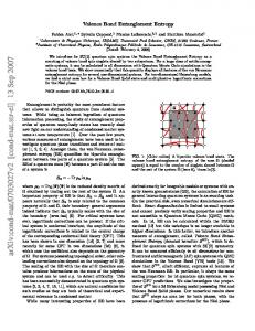
FIG. 2. Consider the simplified setup where we discretize the string to two points X μ ¼ ðxμ1 ; xμ2 Þ. In terms of the center of mass X 0 ¼ 12 ðx1 þ x2 Þ and the separation Y ¼ 12 ðx1 − x2 Þ, we can extend the subregion (in blue) from target space to the entire configuration space in multiple ways. On the left, we count all strings with center of mass in the blue region, while on the right we count all strings which are entirely in the blue region. Note that while the subregion on the left looks non-compact, the string tension implies that the wave function of physical states of the string will be exponentially localized around Y ¼ 0.

066025-10

PHYS. REV. D 97, 066025 (2018)

REMARKS ON ENTANGLEMENT ENTROPY IN STRING THEORY In order to compute the entropy in OSFT, we made a choice for how to extend the entanglement region from the target spacetime to the full configuration space of open strings Mopen —namely, we included all strings with their center of mass inside the subregion. This extension is not unique, and the specific result of the entanglement entropy computation will depend of the choice of extension. For instance, we could have counted all strings which lie entirely within the subregion (see Fig. 2). However, we expect that independent of how we extend the subregion, string theory will soften the UV divergences, and that stringy edge modes should always exist because of the gauge symmetry of string field theory. It is desirable to better understand the dependence of the entanglement entropy on the choice of extension. It might also be interesting to understand the connection of ideas presented in this paper with the studies of causality in string field theory [14,15,47–50]. Another question of interest is the finite gs corrections—entanglement entropy in interacting, non-local theories potentially has an interesting crossover behavior between area law and volume law depending on whether the subregion size is larger or small compared to the scale of non-locality [51–54]. It would be interesting to check whether open string theory exhibits this phenomenon, perhaps perturbatively in gs . The general form of our calculations suggests that in a full open þ closed super-SFT with the correct gauge group the entanglement entropy may be strictly finite. If true that would be very interesting and useful. This may be related generally to the idea of the holographic principle and the idea that the number of d.o.f. in quantum gravity in a finite region should actually be finite. In particular if we consider a black hole, it would be very interesting to understand the entanglement entropy in string theory across the horizon. This was the focus of early attempts to understand the origin of black hole thermodynamics in quantum gravity, but those efforts were carried out in first-quantized string theory using the replica method and were challenged by the presence of off-shell conical backgrounds that may not be well defined [1]. Here we have outlined an approach, albeit in open string field theory, that may allow a precise calculation of entanglement across a horizon that does not face these challenges. For this purpose however, we need to extend this approach to closed string theory. An important subtlety in this case is that the definition of a subregion in a gravitational theory requires an asymptotic boundary or a horizon, since only diffeomorphism invariant constructs are meaningful. We expect therefore that the choice of a subregion in loop space should involve a careful, diffeomorphism invariant construction. Secondly, it is also presently unclear how closed string field theory regulates the ultraviolet divergences in entanglement entropy. Finally, at a more abstract level, we could take the point of view that a consistent string theory is a 2d CFT (with special properties) and that spacetime is a meaningful

concept only in certain special limits. It would be interesting to try to reconcile some of these points with the ideas presented in this paper. ACKNOWLEDGMENTS We would like to thank Pawel Caputa, Falk Hassler, Jonathan Heckman, Arjun Kar, Rob Leigh, Aitor Lewkowycz, Djordje Minic, Charles Rabideau and Tadashi Takayanagi for helpful discussions. Research funded by the Simons Foundation (No. 385592, V. B) through the It From Qubit Simons Collaboration, and the U.S. Department of Energy Contract No. FG02-05ER-41367. APPENDIX: BASIC REVIEW OF COVARIANT STRING FIELD THEORY In this Appendix, we will briefly review Witten’s covariant open string field theory, following [8] (see also [55–57] and references there-in). This is entirely standard material, and is included here only for completeness. The world sheet action is given by Z 1 SX ¼ d2 σ∂ α Xμ ðτ; σÞ∂ α Xμ ðτ; σÞ; ðA1Þ 4π while the ghost action (arising from gauge-fixing the Diff × Weyl gauge symmetries on the world sheet) is given by Z 1 Sgh ¼ d2 σðc− ∂ − bþþ þ cþ ∂ þ b−− Þ ðA2Þ π where ∂  ¼ p1ffiffi2 ð∂ τ  i∂ σ Þ. Open string boundary conditions are cþ ¼ c− and bþþ ¼ b−− at the end points σ ¼ 0, π. With these boundary conditions, both b and c have precisely one zero mode. The BRST current can be written in terms of the world sheet Virasoro generators as: Q ¼ c0 ðL0 − 1Þ þ

X 1X c−n Ln − ðn − mÞ∶c−n c−m bnþm ∶ 2 n;m n≠0 ðA3Þ

where recall that the world sheet-Virasoro generators can be written in terms of the string-oscillator modes as Ln ¼

∞ 1 X ∶α α ∶: 2 m¼−∞ n−m m

ðA4Þ

Note also that following standard convention, we have used the “folding trick” to rewrite the two copies of ghosts (corresponding to ) in terms of a single copy of the chiral closed string modes and then Fourier expanded these in terms of cn and bn .

066025-11

PHYS. REV. D 97, 066025 (2018)

VIJAY BALASUBRAMANIAN and ONKAR PARRIKAR When D ¼ 26, the BRST charge is nilpotent, i.e. Q2 ¼ 0. The quantization of a single string in the BRST formalism is accomplished by requiring the physical Hilbert space to be in the BRST cohomology Qjψi ¼ 0;

ðA5Þ

with two states ψ and ψ 0 considered equivalent if jψ 0 i ¼ jψi þ Qjϵi. Additionally, we also require physical states to be annihilated by all ghost and antighost annihilation operators bn , cm ∀ n; m > 0, and also by b0. Following standard notation, we will denote the physical vacuum in the ghost zero-mode sector by j↓i: b0 j↓i ¼ 0:

ðA6Þ

and assign it ghost number −1=2. Witten’s formulation of open-string field theory (OSFT) is in terms of a noncommutative gauge theory. It is convenient to bosonize the ghosts ðb; cÞ → ϕ in order to introduce this version of OSFT, but for our purposes the details of the ghosts will not be very important, so we do not give all the details of the bosonization map here (see [8] for the relevant details). The gauge field of this noncommutative gauge theory lives in an algebra B, where the elements of B are states of the one-string Hilbert space. Equivalently, one can think of B as consisting of string fields Ψ½Xμ ðσÞ; ϕðσÞ ¼ hXμ ðσÞ; ϕðσÞjΨi

Z Y 2

B ¼⊕∞ n¼−∞ Bn ; where n ¼ G þ 3=2 with G being the ghost number. As explained before, physical states have ghost number G ¼ −1=2 and therefore live in B1 ; consequently we may refer to them as one-forms (more generally n-forms are elements of Bn ). We now describe two operations which will be central to the R construction of the OSFT: (i) Integration, ∶B → C, and (ii) Product, ∶B × B → B. The integration is defined as Z

Z Ψ¼

3i

π

DXμ ðσÞDϕðσÞe− 2 ϕð2Þ

π=2 Y

δ½Xμ ðσÞ − Xμ ðπ − σÞ

σ¼0

ðA7Þ

on Mopen —the space of open-string configurations on target space (plus ghost configurations). Recall that Fourier modes of the string field create and annihilate single string states in the OSFT Hilbert space. The algebra B has a Z-grading

ðΨ  χÞ½Xμ ðσÞ; ϕðσÞ ¼

R FIG. 3. Pictorial representations of the operations and . 3i The black dot with  signs indicates an insertion of e 2 ϕ at the midpoint.

×

π=2 Y

δ½ϕðσÞ − ϕðπ − σÞΨ½Xμ ðσÞ; ϕðσÞ;

ðA8Þ

σ¼0

namely one simply sews together the two halves of the 3i π string with an insertion of the operator e− 2 ϕð2Þ at the midpoint (see Fig. 3). The star product is defined by

DX i Dϕi eþ 2 ϕðπ=2Þ Ψ½Xμ1 ; ϕ1 χ½Xμ2 ; ϕ2  3i

i¼1

×

π=2 Y σ¼0

×

π=2 Y σ¼0

δ½Xμ ðσÞ − Xμ1 ðσÞδ½Xμ1 ðπ − σÞ − X μ2 ðσÞδ½Xμ2 ðπ − σÞ − Xμ ðπ − σÞ δ½ϕðσÞ − ϕ1 ðσÞδ½ϕ1 ðπ − σÞ − ϕ2 ðσÞδ½ϕ2 ðπ − σÞ − ϕðπ − σÞ;

or in other words we sew the right half of the first string with the left half of the second string, this time inserting 3i eþ 2 ϕ at the midpoint (see Fig. 3).11 Some important

ðA9Þ

properties of the noncommutative algebraic structure we have encountered above are listed here: QðA  BÞ ¼ ðQAÞ  B þ ð−1ÞnA A  ðQBÞ;

11

The operator insertions at the midpoint are important to ensure ghost-number conservation.

066025-12

A  ðB  CÞ ¼ ðA  BÞ  C;

ðA10Þ ðA11Þ

PHYS. REV. D 97, 066025 (2018)

REMARKS ON ENTANGLEMENT ENTROPY IN STRING THEORY Z

Z A  B ¼ ð−1Þ

nA nB

B  A;

ðA12Þ

for A; B; C ∈ B. Also, explicit calculation shows that Z Qf ¼ 0 ðA13Þ for any f that vanishes at infinity. It is also worth noting that R the operation Ψ  χ is quite simple: Z Z Ψ  χ ¼ ½DXDϕΨ½Xðπ − σÞ; ϕðπ − σÞχ½XðσÞ; ϕðσÞ:

one. We will work with the free string field, which satisfies QA ¼ 0, and only keep track of the photon in our string field. This amounts to expand the string field up to the first oscillator level and ignoring the tachyon (the zeroth oscillator level): Z jAi ¼

where Aμ corresponds to the photon and f is an auxiliary field (whose origin will become clear below). Using Eq. (A3), the equation of motion is given by  dD k 1 QjAi ¼ ð−ik2 Aμ þ 2kμ fÞαμ−1 c0 ð2πÞD 2  − ðikμ Aμ − 2fÞc−1 j0; k; ↓i ¼ 0: Z

ðA14Þ If we further impose the reality condition Ψ½Xμ ðπ − σÞ; ϕðπ − σÞ ¼ Ψ ½Xμ ðσÞ; ϕðσÞ on the string fields, then it becomes clear that Z Ψ  χ ¼ hΨjχi:

ðA15Þ

ðA18Þ

String interactions appear in the second term. Further, the action is naturally gauge invariant under the infinitesimal gauge transformation

which together of course constitute Maxwell’s equations. The Uð1Þ gauge transformation comes from the following OSFT gauge transformation: Z jAi → jAi þ Qjεi;

jεi ¼

dD k εðkÞb−1 j0; k; ↓i; ð2πÞD ðA22Þ

More explicitly, we find Z Qjεi ¼

  dD k 1 2 μ εðkÞ k c0 b−1 þ kμ α−1 j0; ki; 2 ð2πÞD

ðA23Þ

which of course corresponds to shifting Aμ → Aμ þ ∂ μ ε;

ðA19Þ

where ε ∈ B0 is a zero form (i.e., has ghost number −3=2). Equations (A18) and (A19) linearized around A ¼ 0 give the BRST cohomology conditions on physical states. It is helpful to see how the above equation of motion and gauge symmetry lead to the Maxwell equation and Uð1Þ gauge symmetry in terms of the string-oscillators at level

2f ¼ ∂ μ Aμ ;

□Aμ ¼ 2∂ μ f;

ðA16Þ

The equation of motion corresponding to this action is given by

δε A ¼ Qε þ A  ε − ε  A;

ðA21Þ

The equation of motion therefore imposes

Having defined the algebra B and its attendant operations, Witten wrote down the following action for open string field theory in terms of the string gauge field A ∈ B1 :  Z  1 2 A  QA þ A  A  A : ðA17Þ SOSFT ½A ¼ 2 3 gs

QA þ A  A ¼ 0:

dD k ð−iAμ ðkÞαμ−1 þ fðkÞc0 b−1 Þj0;k;↓i; ðA20Þ ð2πÞD

as expected. Note that in addition, it also shifts f → f þ 12 □ε. It is clear from the above discussion, that the field f is an auxiliary field which upon integrating out leads to the covariant Maxwell theory. We can think of “fixing” f as a choice of gauge-fixing. For example, fixing f ¼ 0 is equivalent to the Lorentz gauge.

066025-13

PHYS. REV. D 97, 066025 (2018)

VIJAY BALASUBRAMANIAN and ONKAR PARRIKAR [1] L. Susskind and J. Uglum, Black hole entropy in canonical quantum gravity and superstring theory, Phys. Rev. D 50, 2700 (1994). [2] A. Dabholkar, Strings on a cone and black hole entropy, Nucl. Phys. B439, 650 (1995). [3] A. Dabholkar, Quantum corrections to black hole entropy in string theory, Phys. Lett. B 347, 222 (1995). [4] S. He, T. Numasawa, T. Takayanagi, and K. Watanabe, Notes on entanglement entropy in string theory, J. High Energy Phys. 05 (2015) 106. [5] T. G. Mertens, H. Verschelde, and V. I. Zakharov, Revisiting noninteracting string partition functions in Rindler space, Phys. Rev. D 93, 104028 (2016). [6] T. G. Mertens, H. Verschelde, and V. I. Zakharov, String theory in polar coordinates and the vanishing of the oneloop Rindler entropy, J. High Energy Phys. 08 (2016) 113. [7] W. Donnelly and G. Wong, Entanglement branes in a twodimensional string theory, J. High Energy Phys. 09 (2017) 097. [8] E. Witten, Noncommutative geometry and string field theory, Nucl. Phys. B268, 253 (1986). [9] E. Witten, Interacting field theory of open superstrings, Nucl. Phys. B276, 291 (1986). [10] W. Donnelly and L. Freidel, Local subsystems in gauge theory and gravity, J. High Energy Phys. 09 (2016) 102. [11] M. Kaku and K. Kikkawa, The field theory of relativistic strings, Pt. 1. Trees, Phys. Rev. D 10, 1110 (1974). [12] M. Kaku and K. Kikkawa, The field theory of relativistic strings. 2. Loops and Pomerons, Phys. Rev. D 10, 1823 (1974). [13] C. B. Thorn, String field theory, Phys. Rep. 175, 1 (1989). [14] E. J. Martinec, The light cone in string theory, Classical Quantum Gravity 10, L187 (1993). [15] D. A. Lowe, Causal properties of string field theory, Phys. Lett. B 326, 223 (1994). [16] H. Hata, H. Oda, and S. Yahikozawa, String field theory in Rindler space-time and string thermalization, Prog. Theor. Phys. 96, 985 (1996). [17] M. Burkardt, Light front quantization, Adv. Nucl. Phys. 23, 1 (1996). [18] I. Peschel, Letter to the editor: Calculation of reduced density matrices from correlation functions, J. Phys. A 36, L205 (2003). [19] H. Casini and M. Huerta, Entanglement entropy in free quantum field theory, J. Phys. A 42, 504007 (2009). [20] D. N. Kabat, Black hole entropy and entropy of entanglement, Nucl. Phys. B453, 281 (1995). [21] J. Polchinski, String Theory, Cambridge Monographs on Mathematical Physics (Cambridge University Press, Cambridge, England, 1998), vol. 1. [22] J. Polchinski, Evaluation of the one loop string path integral, Commun. Math. Phys. 104, 37 (1986). [23] G. Zemba and B. Zwiebach, Tadpole graph in covariant closed string field theory, J. Math. Phys. (N.Y.) 30, 2388 (1989). [24] B. Zwiebach, How covariant closed string theory solves a minimal area problem, Commun. Math. Phys. 136, 83 (1991). [25] B. Zwiebach, Closed string field theory: Quantum action and the B-V master equation, Nucl. Phys. B390, 33 (1993). [26] G. Siopsis, Hamiltonian formulation of string field theory, Phys. Lett. B 195, 541 (1987).

[27] W. Donnelly, Decomposition of entanglement entropy in lattice gauge theory, Phys. Rev. D 85, 085004 (2012). [28] P. V. Buividovich and M. I. Polikarpov, Entanglement entropy in gauge theories and the holographic principle for electric strings, Phys. Lett. B 670, 141 (2008). [29] H. Casini, M. Huerta, and J. A. Rosabal, Remarks on entanglement entropy for gauge fields, Phys. Rev. D 89, 085012 (2014). [30] W. Donnelly and A. C. Wall, Entanglement Entropy of Electromagnetic Edge Modes, Phys. Rev. Lett. 114, 111603 (2015). [31] D. Radicevic, Notes on entanglement in Abelian gauge theories, arXiv:1404.1391. [32] S. Ghosh, R. M. Soni, and S. P. Trivedi, On the entanglement entropy for gauge theories, J. High Energy Phys. 09 (2015) 069. [33] E. Witten, Chern-Simons gauge theory as a string theory, Progress of mathematics 133, 637 (1995). [34] J. R. Fliss, X. Wen, O. Parrikar, C.-T. Hsieh, B. Han, T. L. Hughes, and R. G. Leigh, Interface contributions to topological entanglement in Abelian Chern-Simons theory, J. High Energy Phys. 09 (2017) 056. [35] M. Geiller, Edge modes and corner ambiguities in 3d Chern-Simons theory and gravity, Nucl. Phys. B924, 312 (2017). [36] G. Wong, A note on entanglement edge modes in Chern Simons theory, arXiv:1706.04666. [37] X.-L. Qi, H. Katsura, and A. W. W. Ludwig, General Relationship between the Entanglement Spectrum and the Edge State Spectrum of Topological Quantum States, Phys. Rev. Lett. 108, 196402 (2012). [38] L. A. Pando Zayas and N. Quiroz, Left-right entanglement entropy of boundary states, J. High Energy Phys. 01 (2015) 110. [39] D. Das and S. Datta, Universal Features of Left-Right Entanglement Entropy, Phys. Rev. Lett. 115, 131602 (2015). [40] H. J. Schnitzer, Left-right entanglement entropy, D-branes, and level-rank duality, arXiv:1505.07070. [41] L. A. Pando Zayas and N. Quiroz, Left-right entanglement entropy of Dp-branes, J. High Energy Phys. 11 (2016) 023. [42] I. V. Vancea, Entanglement entropy in the σ-model with the de Sitter target space, Nucl. Phys. B924, 453 (2017). [43] I. V. Vancea, Nonequilibrium dynamics of the σ-model modes on the de Sitter space, Adv. High Energy Phys. 2017, 3706870 (2017). [44] A. Kitaev and J. Preskill, Topological Entanglement Entropy, Phys. Rev. Lett. 96, 110404 (2006). [45] M. A. Levin and X.-G. Wen, String net condensation: A physical mechanism for topological phases, Phys. Rev. B 71, 045110 (2005). [46] S. Dong, E. Fradkin, R. G. Leigh, and S. Nowling, Topological entanglement entropy in Chern-Simons theories and quantum Hall fluids, J. High Energy Phys. 05 (2008) 016. [47] D. A. Lowe, L. Susskind, and J. Uglum, Information spreading in interacting string field theory, Phys. Lett. B 327, 226 (1994). [48] D. A. Lowe, J. Polchinski, L. Susskind, L. Thorlacius, and J. Uglum, Black hole complementarity versus locality, Phys. Rev. D 52, 6997 (1995).

066025-14

REMARKS ON ENTANGLEMENT ENTROPY IN STRING THEORY [49] H. Hata and H. Oda, Causality in covariant string field theory, Phys. Lett. B 394, 307 (1997). [50] T. Erler and D. J. Gross, Locality, causality, and an initial value formulation for open string field theory, arXiv:hep-th/ 0406199. [51] W. Fischler, A. Kundu, and S. Kundu, Holographic entanglement in a noncommutative gauge theory, J. High Energy Phys. 01 (2014) 137. [52] J. L. Karczmarek and C. Rabideau, Holographic entanglement entropy in nonlocal theories, J. High Energy Phys. 10 (2013) 078.

PHYS. REV. D 97, 066025 (2018)

[53] C. Rabideau, Perturbative entanglement entropy in nonlocal theories, J. High Energy Phys. 09 (2015) 180. [54] H. Z. Chen and J. L. Karczmarek, Entanglement entropy on a fuzzy sphere with a UV cutoff, arXiv:1712.09464. [55] D. J. Gross and A. Jevicki, Operator formulation of interacting string field theory (i), Nucl. Phys. B283, 1 (1987). [56] W. Taylor and B. Zwiebach, in Strings, Branes and Extra Dimensions: TASI 2001: Proceedings, 2003, p. 641, https://www.worldscientific.com/doi/abs/10.1142/ 9789812702821_0012. [57] W. Taylor, String field theory, arXiv:hep-th/0605202.

066025-15