Remarks on some open problems in phase-field modelling of ...

arXiv:1004.4502v1 [cond-mat.mtrl-sci] 26 Apr 2010

Remarks on some open problems in phase-field modelling of solidification Mathis Plapp Physique de la Matière Condensée, ´ Ecole Polytechnique, CNRS, 91128 Palaiseau, France April 27, 2010 Abstract Three different topics in phase-field modelling of solidification are discussed, with particular emphasis on the limitations of the currently available modelling approaches. First, thin-interface limits of two-sided phasefield models are examined, and it is shown that the antitrapping current is in general not sufficient to remove all thin-interface effects. Second, orientation-field models for polycrystalline solidification are analysed, and it is shown that the standard relaxational equation of motion for the orientation field is incorrect in coherent polycrystalline matter. Third, it is pointed out that the standard procedure to incorporate fluctuations into the phase-field approach cannot be used in a straightforward way for a quantitative description of nucleation.

1

Introduction

The phase-field method has become the method of choice for simulating microstructure formation during solidification. It owes its popularity mainly to its algorithmic simplicity: the cumbersome problem of tracking moving solid-liquid interfaces or grain boundaries is avoided by describing the geometry in terms of one or several phase fields. The phase fields obey simple partial differential equations that can be easily coded by standard numerical methods. The foundations of the phase-field method and its application to solidification have been the subject of several recent review articles [1, 2, 3, 4, 5, 7, 6], and it seems of little use to repeat similar information here. Instead, in this paper several topics are discussed where robust phase-field modelling tools are not yet available because some fundamental questions remain open. In Sec. 2, the thin-interface limit of two-sided phase-field models is examined, and it is shown that the currently available approaches cannot in general eliminate all effects linked to the finite interface thickness. In Sec. 3, orientation-field models for polycrystalline solidification are discussed, and it is shown that the standard 1

equation of motion usually written down for the orientation field is not appropriate for the evolution of coherent crystalline matter. Finally, in Sec. 4, the inclusion of microscopic fluctuations in the phase-field equations is reviewed, and it is shown that the standard approach cannot be used in a straightforward way to investigate the process of nucleation. The common point of these topics is that they pose challenges or limitations for straightforward computations. Indeed, a characteristic feature of the phase-field method is that its equations can often be written down following simple rules or intuition, but that their detailed properties (which have to be known if quantitative simulations are desired) become only apparent through a mathematical analysis that can be quite involved. Therefore, it is not always easy to perceive the limits of applicability of the method. It is hoped that the present contribution will be helpful to point out some pitfalls and to stimulate further discussions that will facilitate the solution of these issues.

2

Thin-interface limits: antitrapping current and the Kapitza resistance

The precision and performance of phase-field models have been greatly enhanced in the last decade by a detailed control of their properties. Phase-field models are rooted in the mean-field description of spatially diffuse interfaces by order parameters. However, to be useful for simulating microstructure formation in solidification, phase-field models need to bridge the scale gap between the thickness of the physical solid-liquid interfaces and the typical scale of the microstructures. This is achieved by increasing the interface width in the model, sometimes by several orders of magnitude. Obviously, this procedure magnifies any physical effect that is due to the diffuseness of the interface. Therefore, to guarantee precise simulations, all these effects have to be controlled and, if possible, eliminated. The privileged tool to achieve this is the so-called thininterface limit: the equations of the phase-field model are analysed under the assumption that the interface thickness is much smaller than any other physical length scale present in the problem, but otherwise arbitrary. The procedure of matched asymptotic expansions then yields the effective boundary conditions valid at the macroscale, which contain all effects of the finite interface thickness up to the order to which the expansions are carried out. This procedure was pioneered by Karma and Rappel, who analysed the symmetric model of solidification (equal diffusion constants in the solid and the liquid) and obtained a thin-interface correction to the expression of the kinetic coefficient [8]. The use of this result has made it possible to carry out quantitative simulations of free dendritic growth of a pure substance, both at high and low undercoolings [9, 12, 11, 10]. It turned out, however, that the generalisation of this method to a model with arbitrary diffusivities is far from trivial [13], since several new thin-interface effects appear, which cannot all be eliminated simultaneously. A solution to this problem was found later for the case of the

2

one-sided model (zero diffusivity in the solid) with the introduction of the socalled antitrapping current [14], and it was shown that quantitative simulations of alloy solidification are possible with this model [15], including multi-phase [16, 17] and multi-component alloys [18]. Recently, several extensions of the antitrapping current were put forward to generalise the approach to the case of finite diffusivity in the solid [6, 19, 20, 21], and simulations were presented which show that the approach works well for the instability of a steady-state planar interface [19] and for free dendritic growth [20]. However, as will be shown below, this is only a partial solution to the problem of developing a general quantitative model, since there is a second, independent thin-interface effect that cannot be removed by an antitrapping current, namely, the Kapitza resistance. For the sake of concreteness, consider the standard phase-field model for the solidification of a pure substance as discussed in Refs. [9, 13]. The evolution equation for the phase field reads ~ 2 φ + φ − φ3 − λu(1 − φ2 )2 , τ ∂t φ = W 2 ∇

(1)

where φ is the phase field, with φ = 1 and φ = −1 corresponding to solid and liquid, respectively, τ is the relaxation time of the phase field, W is the interface thickness, and λ is a dimensionless coupling constant. The field u is a dimensionless temperature defined by u = (T − Tm )/(L/cp ), where Tm , L and cp are the melting temperature, latent heat, and specific heat, respectively. It is assumed for simplicity that cp is the same in both phases. The temperature is governed by a diffusion equation with a source term, h i 1 ~ D(φ)∇u ~ ∂t u = ∇ + ∂t h(φ). 2

(2)

D(φ) = Dl q(φ),

(3)

Here, h(φ), which satisfies h(±1) = ±1, is a function that describes the release or consumption of latent heat during the phase transition, and D(φ) interpolates between the thermal diffusivities of the liquid and the solid, Dl and Ds ,

where the interpolation function q(φ) satisfies q(1) = Ds /Dl and q(−1) = 1. For simplicity, crystalline anisotropy has not been included in the above model because it is not necessary for the present discussion. Furthermore, the equations have been stated in the language of a two-sided thermal model, but with some modifications (as detailed in Refs. [15, 20]), they also apply to the isothermal solidification of a binary alloy. In this case, u is a dimensionless chemical potential (conjugate to the concentration of one of the alloy components), and D(φ) is the chemical diffusivity. In the following, two simple one-dimensional solutions of these equations will be analysed. The first is a steady-state planar front that propagates with constant velocity V in the positive x direction into a liquid of undercooling ∆ (u → −∆ for x → ∞), and leaves behind a constant temperature. This solution only exists if the liquid is undercooled beyond the hypercooling limit, that is, 3

∆ > 1. The sharp-interface solution to this problem is readily obtained and reads u

= const. = u|−

in the solid (x < 0)

(4)

u

= −∆ + u|+ + ∆ exp(−xV /Dl )

in the liquid (x > 0)

(5)

for an interface located at x = 0 (in the frame moving with the interface). Here, u|− and u|+ are the limit values of the temperature when the interface is approached from the solid and the liquid side, respectively. In the standard formulation of the free boundary problem of solidification, it is assumed that the temperature is the same on the two sides of the interface, u|− = u|+ . Then, the use of the two boundary conditions u|+ = −βV , where β is the linear kinetic coefficient, and V = −Dl ∂x u|+ (the Stefan boundary condition) determines the solution, u|+ = u|− = −∆ + 1 (a simple consequence of heat conservation), and V = (∆ − 1)/β. The phase-field equations can be analysed and related to this sharp-interface solution by the method of matched asymptotic expansions in the limit where the interface thickness W is much smaller than the diffusion length Dl /V . This calculation has been presented in detail in Refs. [9, 13, 15, 20] and will not be repeated here. The essential outcome is that, in general, the two asymptotes of the bulk phases do not correspond to the same temperature. The difference is given, to the lowest order, by Z −∞ Z ∞ h(φ0 ) − 1 2 V h(φ0 ) − 1 dx , (6) dx − + u|− − u|+ = 2 D(φ0 ) D(φ0 ) Dl 0 0 where φ0 (x) is the equilibrium profile of the phase field. The physical interpretation of this temperature jump is trapping: when the diffusivity decreases upon solidification, the heat generated at the rear of the interface gets trapped. In the alloy version of the model, this is nothing but the well-known solute trapping effect. Indeed, in sharp-interface models of alloy solidification the chemical potential exhibits a jump at the interface when solute trapping occurs. In the phase-field model, the temperature profile through the interface is determined by the interplay between the rejection of latent heat and the diffusion away from the interface; therefore, it is natural that the heat source function h(φ) and the diffusivity function D(φ) appear in Eq. (6). Whereas, thus, this discontinuity is physically correct, it generates problems for simulations. To see this, is is sufficient to rewrite Eq. (6) in order to make the relevant scales apparent. Since the only length scale in Eq. (1) is the interface thickness W , the equilibrium solution φ0 is a function only of the reduced variable η = x/W . Using this together with the interpolation of D(φ) given by Eq. (3), Eq. (6) becomes u|− − u|+ = F± =

Z

VW (F− − F+ ) , 2Dl

with

(7)

±∞ 0

[p(φ0 (η)) − p(±1)] dη 4

and

(8)

p(φ) =

h(φ) − 1 . q(φ)

(9)

The temperature jump is thus proportional to the velocity, the interface thickness, and the difference of the two integrals; the latter depends only on the choice of the interpolation functions. If W is the physical interface thickness (a few Angstroms), this effect is negligibly small, but if the interface thickness is increased by a large factor to make simulations feasible, this leads to potentially large errors in the simulations. As discussed in detail in Refs. [13, 14, 15], it is not possible to eliminate this macroscopic discontinuity simply by the choice of appropriate interpolation functions, due to other constraints not discussed here. The solution put forward in Ref. [14] and further developed in Ref. [15] is the introduction of an antitrapping current: Eq. (2) is replaced by ~ D(φ)∇u ~ − ~jat , (10) ∂t u = ∇

where the antitrapping current ~jat is given by

˙ n, ~jat = a(φ)W φˆ

(11)

~ ~ where φ˙ is a shorthand for the time derivative ∂t φ, n ˆ = −∇φ/| ∇φ| is the unit normal vector to the interface, and a(φ) is a new interpolation function. This term induces a current which is directed from the solid to the liquid, and ˙ It thus “pushes” proportional to the interface velocity (through the factor φ). heat from the solid to the liquid side of the interface when the interface moves, and can be used to adjust the temperature jump at the interface. For the one-sided model (Ds = 0) with the standard choices√ h(φ) = φ and q(φ) = (1 − φ)/2, it was shown that a constant a(φ) ≡ 1/(2 2) leads to a vanishing jump in u, because it modifies the function p(φ) in Eq. (8) such that F+ = F− . Thus, continuity of the temperature between the two sides of the interface (local equilibrium) is restored for arbitrary W and V , as long as the asymptotic analysis remains valid. Recently, several authors have put forward generalisations of this approach [6, 20, 21] for arbitrary ratio of the diffusivities. For the case analysed above (that is, the current far inside the solid vanishes), they reduce to the simple prescription that the same expression for the antitrapping current can be used, but with an additional prefactor that can be written as (1 − Ds /Dl ), ˙ n. ~jat = a 1 − Ds W φˆ (12) Dl Indeed, the asymptotic analysis shows [19, 20, 21] that in this way the temperature jump can be eliminated. However, this is not the only thin-interface effect that can arise in the twosided case. To see this, consider now a different situation, namely an immobile interface in a temperature gradient. Such an interface can be easily obtained in 5

experiments by maintaining a pure substance between two walls which are held below and above the melting temperature, respectively. When the interface is stationary, ∂t φ = ∂t u = 0 by definition, and Eq. (2) implies that the system is crossed by a constant heat current flowing from the liquid into the solid, − D(φ)∂x u = −j,

(13)

with j a positive constant. As before, the centre of the interface is located at x = 0, and the solid is located in the domain x < 0. This situation can be analysed without performing a perturbation expansion, since it is sufficient to integrate Eq. (13) to obtain a solution for u, Z x j u(x) = u¯ + dx, (14) 0 D(φ(x)) where u ¯ is the temperature at x = 0. The sharp-interface solution for this case is simply given by u(x) = u|− + (j/Ds ) x u(x) = u|+ + (j/Dl ) x

in the solid in the liquid.

(15) (16)

Matching the asymptotes of the phase-field and sharp-interface expressions, it is straightforward to show that there is again a temperature jump given by Z ∞ Z −∞ 1 1 1 1 dx − dx , − − u|+ − u|− = j D(φ(x)) Dl D(φ(x)) Ds 0 0 (17) this time proportional to the current. If the phase-field profile is replaced by its equilibrium shape, this can be rewritten as u|+ − u|− = with G± =

Z

±∞ 0

jW (G+ − G− ) Dl

1 1 − q(φ0 (η)) q(±1)

(18)

dη.

(19)

This temperature jump corresponds to a surface thermal resistance, also called Kapitza resistance, first found for an interface between liquid helium and metal [22]. Indeed, in a sharp-interface picture it is generally necessary to assign a surface resistance to an interface for a complete description of heat transfer, because transport through an interface can be decomposed into three elementary steps: transport in one bulk phase, crossing of the interface, and transport in the other phase. The surface resistance describes the kinetics associated with the crossing of the interface (its inverse is sometimes referred to as the interfacial transfer coefficient). It is characterised either by the value of the resistance, ( u|+ − u|− )/j, or by a length that is obtained by dividing this resistance by the conductivity of the liquid phase. Here, this characteristic length is simply 6

W (G+ −G− ), which is of the order of the interface thickness. Since this quantity is actually an interface excess of the inverse diffusivity (in complete analogy to the interface excesses for equilibrium quantities obtained by the well-known Gibbs construction), it can also be negative – this does not violate the laws of thermodynamics because the local transport coefficients are strictly positive. If the surface resistance is finite, the temperature in the sharp-interface model is not continuous at the interface, but exhibits a jump that is proportional to the current crossing the interface. In the alloy version of the model, this corresponds to a jump in chemical potential that is proportional to the solute flux [23]. Such discontinuities have been thoroughly investigated [24], and can be measured in experiments [25] and detected in molecular dynamics simulations [26, 27] for solid-liquid interfaces. Thus, like the trapping effect, the surface resistance is a natural effect that is proportional to the interface thickness. If the interface thickness is to be upscaled, it should therefore also be eliminated. However, is is immediately clear that this effect cannot be eliminated by any antitrapping current proportional to φ˙ as given by Eq. (12): since the interface does not move, φ˙ = 0 and the antitrapping current vanishes, independently of the current j that crosses the interface. The authors of both Refs. [20, 21] have recognised the importance of the current j. They have developed generalised expressions for the antitrapping current with coefficients that depend on the value of j. As long as the interface velocity remains non-zero, the formal asymptotic analysis shows that it is still possible to eliminate the temperature jump. However, for a fixed current j, the expressions of the coefficients diverge when V tends to zero, such that the asymptotic analysis is not valid in this limit. Thus, it seems unlikely that this approach can be used as a robust method for simulations. In summary, there exist two independent thin-interface effects, one proportional to V , and one proportional to j. On a very fundamental level, this is just the consequence of the fact that the interface motion is driven by a diffusion equation, which has two independent boundary conditions. The corresponding physical quantities are the currents on the two sides of the interface, or one current and the velocity. A general solution to eliminate both thin-interface effects (which are linearly independent) does not seem to exist at this moment, but the above considerations can at least be used to obtain simple criteria when the prescription of Eq. (12) can be used. Indeed, Eqs. (7) and (18) show that if j ≪ V (note that, since u is dimensionless, j has the dimension of a velocity), the Kapitza effect is much smaller than the trapping effect, and can thus be neglected. This is generally the case for equiaxed dendritic growth, in which the gradients outside the growing dendrite, which determine the growth speed, are much larger than the gradients inside the solid. Indeed, it was shown in Ref. [20] that Eq. (12) works well in this case. However, problems might arise in the case of alloy solidification in a temperature gradient or for multicomponent alloys with widely different solute diffusivities, since in this case large currents of heat or certain solutes may cross an interface whose velocity is controlled by a different diffusion field. Such cases have to be critically examined before 7

simulation results can be trusted.

3

Polycrystalline solidification

The size and shape of the crystalline grains formed upon solidification is one of the most important factors that determine materials properties. Therefore, phase-field models that are to be helpful for materials design must be capable of dealing with the evolution of polycrystals, both during solidification of individual columnar or equiaxed grains from the melt and during the subsequent evolution of the grain structure after impingement. This can be achieved using the multi-phase-field approach [28, 29, 30, 31, 33, 32], in which each grain is represented by a different phase field, even if they are of the same thermodynamic phase. The properties of each individual grain boundary or interface can then be specified separately [31], and it has been demonstrated that good quantitative control of the grain boundary properties can be achieved [32]. The problem of handling several hundreds or even thousands of phase fields simultaneously can be solved by recognising that only a small number of fields are important at any given point of space (see for example [34]). An alternative approach is the orientation-field method. Its starting point is the remark that it would be desirable, both for efficiency and simplicity, to formulate a model that works only with a small number of field variables. Indeed, the orientation of a crystal can be described by one scalar quantity (an angle) in two dimensions, and three scalars in three dimension (for instance, the Euler angles). Orientation-field models for pure substances in two dimensions that work with a single phase field, an orientation field (the local angle of the crystalline structure with respect to a fixed coordinate system), and the temperature field were put forward in Refs. [35, 36], and generalised for alloy solidification [3] and to three dimensions [37, 38]. While these models are elegant and simple in their formulation and therefore hugely appealing, it is pointed out here that the evolution equation of the angle field, which takes the form of a simple relaxation equation, does not correctly describe the microscopic evolution of the orientation field since it does not take into account the connectivity of matter and the resulting geometrical conservation laws. For simplicity, anisotropy and crystallographic effects will again be neglected, and it is sufficient to consider a two-dimensional system. The dimensionless free energy of the orientation-field model is [36] Z 2 2 ǫ2 2 W ~ ˜ ~ ~ F= ∇φ + s˜ g(φ) ∇θ + h(φ) ∇θ + f (φ, u) d~r, (20) 2 2

where now φ = 0 and φ = 1 in the liquid and the solid, respectively, s and ˜ ǫ are positive constants, g˜(φ) and h(φ) are monotonous functions that satisfy ˜ ˜ g˜(0) = h(0) = 0 and g˜(1) = h(1) = 1, and f (φ, u) is the local free energy density, with u the same dimensionless temperature field as previously; the standard choice is f (φ, u) = φ2 (1 − φ)2 + λu(10φ3 − 15φ4 + 6φ5 ). Recently, an 8

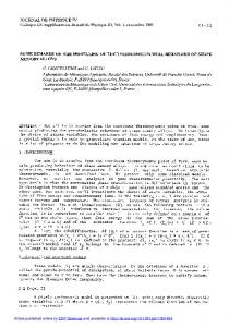
Figure 1: Evolution of a tricrystal in the orientation-field models. The crystalline slab in the centre rotates, and eventually the grain boundaries disappear.

alternative model was developed [39], Z 2 2 W 7φ3 − 6φ4 ~ 2 ~ ∇φ + ν ∇θ + f (φ, u) d~r, F= 2 (1 − φ)2

(21)

where ν is a constant. In the following, these models will be called model I and model II. They both have some features that distinguish them from standard ~ phase-field models. Model I contains a term proportional to |∇θ|, which has ~ a singular derivative at |∇θ| = 0. Model II has only a regular square gradient ~ but it is multiplied by a singular function of the phase field φ, which term in ∇θ, diverges in the limit φ → 1 (the solid). These singular features are needed to create stable grain boundary solutions, that is, localised spatial regions where the phase field departs from its solid value and the angle field exhibits rapid variations. Both models have a variational structure for the dynamics of the phase field and the angle field, that is δF , (22) ∂t φ = −Mφ δφ δF , (23) δθ which means that both φ and θ evolve such as to follow the gradient of the free energy, with Mφ and Mθ being the corresponding mobilities (which may be functions of the fields). In the following, it will be shown that Eq. (23) is incorrect for coherent crystalline matter. To illustrate the problems with this equation of motion, it is again useful to analyse a simple one-dimensional situation, which is a tricrystal. A slab of crystalline orientation θ0 is sandwiched between two crystals of identical orientation θ = 0, as shown in the left side of Fig. 1. The two crystals on the sides of the system are assumed to be clamped to a substrate, that is, θ = 0 for all times. In both models, this initial condition evolves with time: the orientation of the central slab remains homogeneous, but changes with time to approach the orientation of the outer crystals. The final state is a uniform solid of orientation θ = 0: the central slab has disappeared. ∂t θ = −Mθ

9

Of course, this process can take place since it corresponds to a minimisation of the free energy: the two grain boundaries with their positive grain boundary energy are eliminated. However, the pathway of this dynamics is not appropriate for the evolution of a coherent crystal. In fact, Eq. (23) corresponds to the dynamics of matter which has orientational, but no positional order, such as a ~ is omitted liquid crystal. Indeed, if in model I the term proportional to |∇θ| or in model II the singular coupling function is replaced by a regular one, the resulting model can be mapped to the standard Landau-de Gennes model for nematic liquid crystals in two dimensions [40]. The free energies in Eqs. (20) and (21) have been designed to stabilise grain boundaries, which do not exist in a nematic liquid crystal. The energetics of the models are thus quite different from liquid crystals. In contrast, the type of the dynamics has stayed the same. To understand where is the difference in dynamics between liquid crystals and crystals, consider the elongated molecules of a nematic liquid crystal characterised by a director field of a certain orientation θ0 . Since the molecules have no bonds, it is possible to change the local orientation while keeping the centres of mass fixed, by just making each molecule rotate around its centre of mass (of course, in a dense liquid crystal, this exact procedure is not possible because of steric exclusion, but the director can still be changed with only short-range displacements of the centres of the molecules). The system is thus free to locally change orientation in order to lower its free energy, and thus follows Eq. (23). This is obviously not the case in crystalline matter: it is not possible to rotate a unit cell without displacing the surrounding neighbours, because bonds (or, more generally, the positional ordering of elements) define a connectivity. It is easy to grasp that the evolution depicted in Fig.1 is impossible if the connectivity of the central slab is preserved. Thus, a consistent evolution equation for θ has to take into account this connectivity, or, in other words, the evolution of the positions. This is, in general, a complicated undertaking. Two elementary situations where it easy to obtain an equation are (i) rigid body rotation, in which case the (advected) time derivative of the local angle is given by the curl of the local velocity field, or (ii) purely elastic deformations of the solid, in which case the orientation is not an independent quantity but can be deduced from the elastic displacement field. Here, a third possibility will be briefly discussed, namely, plastic deformation. This corresponds precisely to a change in the connectivity of matter. If the matter in question can be considered reasonably crystalline (as opposed to, for example, an amorphous material), its geometry can formally always be described by a density of dislocations, which are singularities of the displacement field if a perfect crystal is taken as the reference state. If, furthermore, grain boundaries remain coherent (that is, no grain boundary sliding takes place), the evolution of the local orientation can be linked to the motion of dislocations. A complete description is far outside of the scope of this article; the interested reader is referred to Ref. [41] for a detailed introduction to the continuum theory of defects. Here, only two simple examples will be qualitatively treated for illustration. 10

Figure 2: Sketch of the elementary process that generates a rotation of the central crystal slab by the motion of a single edge dislocation. Only the crystal planes close to the vertical direction are shown.

Consider again the tricrystal configuration. In the sketch shown in Fig. 2, only one set of crystal planes is shown for clarity, and the central slab has a small misorientation with respect to the outer crystals. In this situation, the two lowangle grain boundaries consist of individual edge dislocations. The inner crystal can now rotate by an elementary process: take one of the edge dislocations of the left grain boundary (marked by a circle) and make it glide towards the other grain boundary. This process involves only local reconnection events. When the dislocation arrives at the right grain boundary, it can annihilate with a dislocation of the opposite sign. As a result, one dislocation has disappeared from each grain boundary. Of course, this process can repeat itself until no dislocation is left, and the grain boundaries have disappeared. It should be stressed that this pathway for rearrangement exhibits large energy barriers, since the elastic energy of a single dislocation is much higher in the centre of the slab than at its original position within the grain boundary. Therefore, if only thermal fluctuations are driving this process (no external strains), it will be extremely slow. On a more quantitative level, the misorientation through a grain boundary is linked to the density of dislocations by simple geometrical arguments. Therefore, it is natural that the misorientation is lowered when the dislocation density in the grain boundaries decreases. Furthermore, it is obvious that the rotation rate of the central slab is proportional to the current of dislocations crossing the crystal. Thus, a consistent equation of motion for the orientation should be based on the evolution of the dislocation density. However, the development of such an equation is a difficult task, because the motion of dislocations is determined by their complicated elastic interactions, as well as by external strain and interactions with other defects. Despite intense activity on the phase-field modelling of defects, elasticity, and plasticity (see [42] for a recent overview), such an equation seems at present out of reach. Let us now come back to the outcome of the simulations for the tricrystal configuration. The functional derivative of the gradient term in Eq. (20) of model I generates a non-local diffusion equation for the angle field, which has 11

to be regularised as described in Ref. [36]. For a constant mobility, the nonlocal interaction between the grain boundaries leads to a rotation rate that is almost independent of the distance between the grain boundaries. In model II, the rotation rate of the central crystal decreases exponentially with the distance between the grain boundaries [43]. In both cases, the central slab eventually disappears. While, quantitatively, neither of these evolutions is likely to be accurate, qualitatively the result is the same as the one achieved by dislocation motion. To see that there can be qualitative differences between the two dynamics, consider now a circular grain of orientation θg inserted in an infinite monocrystal of orientation θ = 0. Suppose that the misorientation (which is equal to θg ) is small, such that the grain boundary is made of individual dislocations separated by a typical distance d which is much larger than the lattice spacing. Furthermore, suppose that the grain radius R is large, R ≫ d, such that on the scale of the grain the boundary can still be described as a continuous line. For simplicity, disregard any anisotropy in the grain boundary energy or mobility. Then, the grain will shrink by standard motion by curvature, and the dislocations will simply move towards the centre of the grain. Note that the motion of the dislocations might not be strictly radial due to their coupling to the crystal structure; however, this does not change the present discussion, as long as no annihilation of dislocations takes place. Indeed, in this case, the total number of dislocations is conserved, and the dislocation density is simply proportional to 1/R, which increases with time as the grain shrinks. This means that the misorientation also increases with time, and if the outer crystal is fixed, the circular inner grain has to perform a rigid body rotation away from the orientation of the outer crystal. This seems surprising at first, since for low-angle grain boundaries the grain boundary energy is an increasing function of the misorientation. However, this process is perfectly possible if it leads to a decrease of the total energy of the grain boundary, which is given by Egb = 2πγ(θg )R, with γ(θg ) the misorientation-dependent grain boundary energy. Its time derivative is dEgb dR dθg ′ = 2π γ(θg ) + Rγ (θg ) , (24) dt dt dt where γ ′ > 0 is the derivative of γ with respect to the misorientation. The evolution can thus take place if the first term, which is always negative since dR/dt < 0, is large enough to outweigh the second one, which is positive. In that case, the geometrical constraints thus predict an increase of θg with time. The orientation-field models make exactly the opposite prediction: since the angle field evolves locally such as to lower the energy, the misorientation of the inner grain should decrease with time. Recently, this situation was investigated by numerical simulations [44] using the phase-field crystal model [45], which gives a faithful microscopic picture of dislocations. An increase of the misorientation with time was observed, consistent with the geometrical constraints. A previous study that had compared phase-field and molecular dynamics simulations [46] and had reached different conclusions was limited to high misorientations, such

12

that the above hypotheses were not satisfied. In conclusion, the simple relaxation equation for the angle field, Eq. (23) is not consistent with the coherent crystalline structure of matter, and can sometimes lead to predictions that are even qualitatively wrong. For practical purposes, the quantitative importance of the committed errors might be small when the evolution of a large-scale grain structure is considered, but this has to be confirmed for each case at hand. It is worth mentioning that orientation-field models have been used to investigate the interplay between the positional and orientational degrees of freedom during the solidification of spherulites [47] or in the presence of foreign-phase particles [48]. These studies were performed with a vanishing orientational mobility Mθ in the solid, and are thus not affected by the problem pointed out here. Indeed, in the interfacial region where the structure of the solid in not yet fully established, the concept of a rotational mobility is valid.

4

Fluctuations and nucleation

Many phase-field simulations include fluctuations, which are often introduced in a purely qualitative way to trigger instabilities or to create some disorder in the geometry of the microstructures. The role of fluctuations has been investigated more quantitatively in connection with the formation of sidebranches in free dendritic growth [49, 50, 10]. The standard approach is to include fluctuations as Langevin terms in the field equations, with coefficients deduced from the fluctuation-dissipation theorem. Before proceeding further, this procedure will be summarised. After inclusion of noise, Eqs. (1) and (2) for the solidification of a pure substance become (see Ref. [49] for details) ~ 2 φ + φ − φ3 − λu(1 − φ2 )2 + ξ(~r, t), ∂t φ = ∇

(25)

~ 2 u + 1 ∂t h(φ) − ∇ ~ · ~q(~r, t), ∂t u = D∇ (26) 2 where D(φ) ≡ D is assumed (symmetric model), and lengths and times have been scaled by the interface thickness W and the phase-field relaxation time τ , respectively. Here, ξ(~r, t) and ~q(~r, t) are random fluctuations of the phase field and random microscopic heat currents, respectively. They are assumed to be δ-correlated in space and time, hξ(~r, t)ξ(~r′ , t)i = 2Fφ δ(~r − ~r′ )δ(t − t′ ),

(27)

hqm (~r, t)qn (~r′ , t)i = 2DFu δnm δ(~r − ~r′ )δ(t − t′ ),

(28)

with dimensionless amplitudes Fφ and Fu given by Fu =

d0 W

d

13

Fexpt ,

(29)

√ d−1 2 2 d0 Fφ = Fexpt , 3 W

(30)

where d is the spatial dimension, and the quantity Fexpt is determined by materials properties only, 2 kB Tm cp , (31) Fexpt = 2 L dd0 where kB , Tm , cp , L, and d0 are Boltzmann’s constant, the melting temperature, the specific heat, the latent heat, and the capillary length, respectively. The latter is given by d0 = γTm cp /L2 , where γ is the surface free energy. With the help of this expression for the capillary length, Fexpt can be rewritten as Fexpt = kB Tm /(γdd−1 ), which makes its physical meaning more transparent: it 0 is the ratio of the thermal energy and a capillary energy scale, and can thus be seen as a non-dimensional temperature. In a finite-difference discretization of timestep ∆t and grid spacing ∆x, the noise terms are implemented by drawing, at each grid point i and for each time step t, independent Gaussian random variables of correlation D

′

ξit ξit′

E

=

2Fφ δii′ δtt′ , (∆x)d ∆t

(32)

where δii′ and δtt′ are now Kronecker symbols, and similarly for ~q. This procedure was shown to yield the correct interface fluctuations at equilibrium in numerical simulations [49]. An obvious question then arises, namely, can this method also be used to explore nucleation ? Phase-field methods have been used recently to investigate homogeneous and heterogeneous nucleation, both in single-phase and multiphase systems (see, for example, [51, 55, 52, 53, 54]). In particular, it was found that for high undercoolings, diffuse-interface models yield better agreement with experiments than classical nucleation theory, since the size of the nuclei is not much larger than the thickness of the diffuse interfaces; therefore, the free energy barriers calculated in phase-field models can differ significantly from classical nucleation theory. Is it sufficient, then, to add thermal noise as described above to obtain quantitative simulations of nucleation processes ? The answer to this question is negative. The reason is that, for strong noise, field equations like the phase-field model are renormalized by the fluctuations. This is a well-known fact in statistical field theory, but its implications do not yet seem to have been fully appreciated in the phase-field community. Therefore, it is useful to briefly sketch a few calculations that can be found in textbooks (see, for example, [56]). They are, therefore, neither new nor complete; however, they will prepare the ground for understanding the conclusions on the phasefield method at the end of this section. Instead of the full phase-field model, consider a single equation for a scalar field φ that reads δH ∂t φ = − + ξ(~r, t), (33) δφ

14

where ξ is a non-conserved noise that is δ-correlated, hξ(~r, t)ξ(~r′ , t′ )i = 2T δ(~r − ~r′ )δ(t − t′ ),

(34)

with T a suitably non-dimensionalized temperature (such as Fexpt , see the discussion after Eq. (31)), and the deterministic part of the equation derives from the functional Z 1 H= (∇φ)2 + V (φ) d~r, (35) 2

where V (φ) is a local potential of the field φ (lengths, times, and energies are dimensionless). It is important to stress that H is not a free energy functional, but the Hamiltonian of the field theory. Eq. (33) generates an evolution in which each microscopic field configuration appears with probability P = Z −1 exp(−H/T ) in the limit of infinite evolution time. Here, Z is the partition function, Z Z= Dφ exp(−H/T ),

(36)

(37)

and Dφ denotes a functional integration over the field φ. The free energy is then obtained by the standard formula F = −T ln Z. The free energy can be calculated exactly for the case of a quadratic potential, V (φ) = m2 φ2 /2, where m is a constant. To carry out the calculations, it is useful to consider a discrete version of the model. For simplicity, consider as the domain of integration V a d-dimensional torus of size Ld with periodic boundary conditions. When this system is discretized with the usual finite difference formulae using N grid points in each direction and hence a grid spacing ∆x = L/N , the integral in Eq. (35) becomes a sum over a finite number of variables. In one dimension, " # 2 N −1 X φn+1 − φn 1 2 2 + m φn , (38) H = ∆x 2 ∆x n=0 with the convention that φN ≡ φ0 . For the discretized system, the functional integration in Eq. (37) is replaced by a simple integration over the field variables at each grid point, Z N −1 Y Z = exp (−H/T ) dφn . (39) n=0

Since the Hamiltonian of Eq. (38) is a quadratic form in the φn ’s, this is a N dimensional Gaussian integral which can be evaluated using standard formulae. The most convenient way is to use a discrete Fourier transform to find the eigenvalues of the quadratic form. The final result for the free energy is (up to a constant that can be dropped) N −1 T X 4 2 πl 2 F= . (40) sin ln m + 2 (∆x)2 N l=0

15

For dimensions d > 1, the same calculation can be repeated without difficulties, and the result is ! d T X 4 X 2 πli 2 F= , (41) sin ln m + 2 (∆x)2 i=1 N li

where the sum is now over an independent index li for each dimension (i = 1 . . . d), and is normally taken over the first Brillouin zone, li ∈ {−N/2+1, N/2}. For an arbitrary potential V (φ), an exact calculation is generally impossible. Statistical field theory has developed sophisticated approximation methods, in particular perturbation expansions. Formally, every potential can be written as a perturbation of a quadratic potential. The perturbation expansion (where the expansion parameter is the temperature, which sets the fluctuation strength) is cumbersome and usually visualised in terms of diagrams [56]. Fortunately, the first order result can be understood in a relatively simple manner if we are interested in homogeneous systems. More precisely, consider the spatial average of the field, Z ¯ = 1 φ(~r, t) d~r, (42) φ(t) Ld which is a fluctuating quantity. The probability distribution of φ¯ can be written as ¯ ∼ exp −Ld f (φ)/T ¯ P (φ) , (43) ¯ is the free energy density. To first order in the perturbation expanwhere f (φ) sion, ! d X X T πl 4 i ¯ = V (φ) ¯ + ¯ + , (44) f (φ) sin2 ln V ′′ (φ) 2Ld (∆x)2 i=1 N li

¯ is identical to the where the correction to the original (“bare”) potential V (φ) exact result for the quadratic potential, with the constant m2 replaced by the ¯ This results from a quadratic second derivative of the bare potential, taken at φ. ¯ approximation (second-order Taylor expansion) of the bare potential around φ. ¯ ¯ The result f (φ) is a renormalized potential for φ. These calculations can be readily verified numerically. As an example, the standard double-well potential was used, V (φ) = −φ2 /2 + φ4 /4 (usually called φ4 -potential in the field-theory literature), and simulated in a two-dimensional system of size L = 32 with a grid spacing of ∆x = 0.5 and T = 0.05, using the standard discretization method described above with a timestep ∆t = 0.005, and an initial condition φ(~r, 0) = 1. In time intervals of 10, φ¯ was calculated, and in total 1000 points were sampled. Then, the free energy can be obtained ¯ and taking the logarithm of the counts by making a histogram of the values of φ, (the normalisation contributes only a constant to f and can be disregarded). The comparison between the simulation and the prediction of Eq. (44) in Fig. 3 shows excellent agreement. It can be seen that the minimum of the free energy density is shifted with respect to its “bare” value φ¯ = 1. This can be understood intuitively by the 16

simulation theory

f

0,0004

0,0002

0 0,95

0,96

0,97

φ

0,98

0,99

1

Figure 3: Renormalized free energy density of the standard double-well potential as calculated from Eq. (44) and from numerical simulations, for T = 0.05, ∆x = 0.5, ∆t = 0.005. Only the part close to one of the potential wells is shown. The zero of f was chosen at the minimum of the renormalized potential. The bin size for the histograms was ∆φ¯ = 0.01.

following reasoning. The system starts in the well of the “bare” potential, at φ¯ = 1. The random fluctuations push the system in both directions with equal probability, but since the potential is asymmetric, the restoring force is larger for fluctuations towards φ¯ > 1 than towards φ¯ < 1; therefore, smaller values are more likely to occur. In the example chosen here, the shift is small (the minimum is close to 1), but for increasing temperature, the correction becomes larger and larger (for an example of such simulations, see [57]), and eventually a phase transition occurs (the double well disappears); in this regime, of course the first-order perturbation result is inaccurate. The correction also depends on the discretization. This is physically sound: a finer discretization introduces more degrees of freedom per unit volume in the discretized system, and hence allows for more fluctuation modes that contribute to the free energy. With a slight change of perspective, this can also be seen as the natural result of a coarse-graining procedure. Indeed, if the free energy is calculated from a given microscopic model by coarse-graining (averaging) over cells with a certain size ∆x larger than the size of the microscopic elements, both the free energy density and the amplitude of the fluctuations that remain after the averaging (which thus have a wavelength larger than ∆x) depend on the choice of ∆x, as was recently demonstrated explicitly for a simple lattice gas model [58]. However, a problem arises in the continuum picture: it is easy to verify that, when the grid spacing ∆x tends to zero, the sum in Eq. (44) diverges for d ≥ 2. This is a classical example of an ultraviolet divergence. Thus, Eq. (33) has no continuum limit, and if it is written down in continuum language, it is implicitly understood that an ultraviolet cutoff must be specified. A reasonable physical value for a cutoff in condensed-matter systems is the size of an atom. 17

Let us now discuss the implications of these facts for phase-field modelling. Even though the above calculation have not been carried out for the full model (φ and u), it is clear that renormalization occurs. If a phase-field model is seen as a simulation tool for a problem that is defined in terms of macroscopic parameters, the relevant quantities that need to be adjusted in the model are the renormalized ones. For instance, thermophysical properties are usually interpolated assuming that the phase field takes fixed values in the bulk phases (φ = ±1). If, on average, this is no longer the case, such as in the example of Fig. 3, these interpolations become incorrect. An obvious idea to cure this problem is to choose the “bare” potential such that the renormalized potential has the desired properties. For the φ4 -potential, which is renormalizable, one may choose V =−

1 + ǫ2 2 1 + ǫ4 4 φ + φ , 2 4

(45)

and determine the constants ǫ2 and ǫ4 by the two conditions f ′ (1) = 0 and f ′′ (1) = 2 using Eq. (44). For the example shown above, the values ǫ2 = 0.0693524 and ǫ4 = 0.0208810 indeed restore the correct bulk properties. However, in a quantitative phase-field model, the macroscopic properties not only of the bulk phases, but also of the interfaces need to be controlled. It is far from obvious that the above procedure, designed for homogeneous systems, will work. This is even more so for the critical nucleus needed to evaluate the nucleation barrier. It is instructive to examine some orders of magnitude. In Nickel, the value of Fexpt is 0.234 [10], of order unity; it can be expected that this value is of similar order of magnitude for other substances with microscopically rough interfaces. An inspection of Eqs. (27–29) reveals that if phase-field simulations are carried out with the “natural” interface thickness, which is of the order of the capillary length d0 , the fluctuations are of order unity (recall that Fφ and Fu are equivalent to T in the numerical example), and renormalization cannot be neglected. This is a natural consequence of the fact that real solid-liquid interfaces do indeed exhibit very strong fluctuations, as evidenced from molecular dynamics simulations [59]; therefore, a mean-field approximation (such as the phase-field model without noise) is not accurate. In contrast, if (as in Refs. [49, 10]) a much larger interface thickness is used, the fluctuation strength is greatly reduced, and the difference between “bare” and renormalized free energy is small. Note, however, that even in this limit a sufficient refinement of the grid would create noticeable fluctuation corrections. We are thus faced with the conclusion (opposite to the usual point of view in phase-field modelling) that the use of the simple prescription of Ref. [49] is more precise for larger interface thickness and coarser grids. It is noted in passing that the concept of the sharp-interface limit, central for the asymptotic analysis in the deterministic case, has to be reexamined because a new length scale (the microscopic cutoff for the fluctuations) has been introduced. In conclusion, it is clear that the use of the phase-field method with fluctuations is subject to caution, at least on small length scales. To gain a better 18

understanding, the fluctuation effects on the couplings of the phase-field variables need to be investigated. Furthermore, a good control of the discretization effects needs to be achieved; the introduction of a simple cutoff will most likely be insufficient, since the renormalized free energy of Eq. (44) also depends on the grid structure. While a large body of results on these topics can certainly be found in the field-theory literature, the development of quantitative models for specific materials remains a challenging task.

5

Conclusions

In this paper, some open questions concerning various aspects of phase-field modelling of solidification have been discussed, and potential future directions of research have been outlined. The selection of topics is necessarily incomplete, both concerning the problems and the potential solutions. For instance, the rapid development of the phase-field crystal approach [45] and related methods currently opens up interesting new perspectives for the modelling of polycrystals, which are not discussed further here. The common point of the topics treated here is that they illustrate the dual nature of the phase-field method. On the one hand, it is a genuine representation of condensed-matter systems and their evolution in terms of order parameters on a mesoscopic scale. On the other hand, with the help of mathematical analysis, it can be turned into an efficient simulation tool for the solution of free boundary problems. As in the past, the development of more efficient and robust models for materials modelling will most likely benefit from the pursuit and confrontation of both of these two complementary viewpoints. Therefore, the further development of the phase-field method remains an exciting research topic at the frontiers of physics, mathematics, and materials science.

Acknowledgements I thank Jean-Marc Debierre, Tristan Ducousso, Alphonse Finel, László Gránásy, Hervé Henry, Alain Karma, Yann Le Bouar, Jesper Mellenthin, Tamás Pusztai, and James Warren for stimulating discussions on these and many other topics.

References [1] W.J. Boettinger, J.A. Warren, C. Beckermann and A. Karma, Annu. Rev. Mater. Res. 32 (2002) p.163–194. [2] L.Q. Chen, Annu. Rev. Mater. Res. 32 (2002) p.113–140. [3] L. Gránásy, T. Pusztai and J.A. Warren, J. Phys. – Cond. Mat. 16 (2004) p.R1205. [4] M. Plapp, J. Cryst. Growth 303 (2007) p.49–57. 19

[5] I. Singer-Loginova and H.M. Singer, Rep. Prog. Phys. 71 (2008) p.106501. [6] I. Steinbach, Model. Simul. Mater. Sci. Eng. 17 (2009) Art-No.073001. [7] H. Emmerich, Adv. Phys. 57 (2008) p.1–87. [8] A. Karma and W.J. Rappel, Phys. Rev. E 53 (1996) p.R3017–R3020. [9] A. Karma and W.J. Rappel, Phys. Rev. E 57 (1998) p.4323–4349. [10] J. Bragard, A. Karma, Y.Y. Lee and M. Plapp, Interface Science 10 (2002) p.121–136. [11] A. Karma, Y.H. Lee and M. Plapp, Phys. Rev. E 61 (2000) p.3996–4006. [12] N. Provatas, N. Goldenfeld and J. Dantzig, J. Comput. Phys. 148 (1999) p.265–290. [13] R.F. Almgren, SIAM J. Appl. Math. 59 (1999) p.2086–2107. [14] A. Karma, Phys. Rev. Lett. 87 (2001) Art-No.115701. [15] B. Echebarria, R. Folch, A. Karma and M. Plapp, Phys. Rev. E 70 (2004) Art-No.061604. [16] R. Folch and M. Plapp, Phys. Rev. E 68 (2003) Art-No.010602(R). [17] R. Folch and M. Plapp, Phys. Rev. E 72 (2005) Art-No.011602. [18] S.G. Kim, Acta Mater. 55 (2007) p.4391–4399. [19] A. Gopinath, R.C. Armstrong and R.A. Brown, J. Cryst. Growth 291 (2006) p.272–289. [20] M. Ohno and K. Matsuura, Phys. Rev. E 79 (2009) Art-No.031603. ´ de la solidification dirigée par la méthode du champ [21] T. Ducousso, Etude de phase : comparaison théorie–expérience pour un alliage binaire dilué, Ph.D. thesis, Université Paul Cézanne, Marseille, France, 2009. [22] P. L.Kapitza, Zh. Eksp. Teor. Fiz. 11 (1941) p.1. [23] P. Maugis and G. Martin, Phys. Rev. B 49 (1994) p.11580–11587. [24] E.T. Swartz and R.O. Pohl, Rev. Mod. Phys. 61 (1989) p.605–668. [25] P.E. Wolf, D.O. Edwards and S. Balibar, J. Low Temp. Phys. 51 (1983) p.489–504. [26] J.L. Barrat and F. Chiaruttini, Mol. Phys. 101 (2003) p.1605–1610. [27] L. Xue, P. Keblinski, S.R. Phillpot, S.U.S. Choi and J.A. Eastman, J. Chem. Phys. 118 (2003) p.337–339. 20

[28] I. Steinbach, F. Pezzolla, B. Nestler, M. Seeßelberg, R. Prieler, G.J. Schmitz and J.L.L. Rezende, Physica D 94 (1996) p.135–147. [29] D. Fan and L.Q. Chen, Acta Mater. 45 (1997) p.611–622. [30] H. Garcke, B. Nestler and B. Stoth, SIAM J. Appl. Math. 60 (1999) p.295– 315. [31] I. Steinbach and F. Pezzolla, Physica D 134 (1999) p.385–393 [32] N. Moelans, B. Blanpain and P. Wollants, Phys. Rev. B 78 (2008) ArtNo.024113. [33] J. Eiken, B. Böttger and I. Steinbach, Phys. Rev. E 73 (2006) ArtNo.066122. [34] L. Vanherpe, N. Moelans, B. Blanpain and S. Vandewalle, Phys. Rev. E 76 (2007) Art-No.056702. [35] R. Kobayashi, J.A. Warren and W.C. Carter, Physica D 140 (2000) p.141– 150. [36] J.A. Warren, R. Kobayashi, A.E. Lobovsky and W.C. Carter, Acta Mater. 51 (2003) p.6035–6058. [37] T. Pusztai, G. Bortel and L. Gránásy, Europhys. Lett. 71 (2005) p.131–137. [38] R. Kobayashi and J.A. Warren, Physica A 356 (2005) p.127–132. [39] J. Mellenthin, Phase-field modelling of polycrystalline solidification, Ph.D. ´ thesis, Ecole Polytechnique, Palaiseau, France, 2007. [40] P.-G. de Gennes and J. Prost, The physics of liquid crystals – second edition, Clarendon Press, Oxford, UK, 1993. [41] E. Kröner, Continuum theory of defects, R. Balian, M. Kléman and J.P. Poirier, eds., Les Houches Session XXXV, North Holland, Amsterdam, 1981, pp. 215–313. [42] Y. Wang and J. Li, Acta Mater. 58 (2010) p.1212–1235. [43] H. Henry, J. Mellenthin and M. Plapp (2010), unpublished. [44] K.A. Wu and P. Voorhees (2010), unpublished. [45] K.R. Elder and M. Grant, Phys. Rev. E 70 (2004) Art-No.051605. [46] M. Upmanyu, D.J. Srolovitz, A.E. Lobkovsky, J.A. Warren and W.C. Carter, Acta Mater. 54 (2006) p.1707–1719. [47] L. Gránásy, T. Pusztai, G. Tegze, J.A. Warren and J.F. Douglas, Phys. Rev. E 72 (2005) Art-No.011605. 21

[48] L. Gránásy, T. Pusztai, J.A. Warren, J.F. Douglas, T. Börzsönyi, and V. Ferreiro, Nature Materials 2 (2003) p.92–96. [49] A. Karma and W.J. Rappel, Phys. Rev. E 60 (1999) p.3614–3625. [50] T. Börzs¨ onyi, T. T´ oth-Katona, A. Buka and L. Gránásy, Phys. Rev. Lett 83 (1999) p.2853–2856; Phys. Rev. E 62 (2000) p.7817–7827. [51] L. Gránásy, T. Börzs¨ onyi and T. Pusztai, Phys. Rev. Lett. 88 (2002) ArtNo.206105. [52] R. Siquieri and H. Emmerich, Philos. Mag. Lett. 87 (2007) p.829–837. [53] L. Gránásy, T. Pusztai, D. Saylor and J.A. Warren, Phys. Rev. Lett. 98 (2007) Art-No.035703. [54] J.A. Warren, T. Pusztai, L. Környei and L. Gránásy, Phys. Rev. B 79 (2009) Art-No.014204. [55] G.I. Toth and L. Gránásy, J. Chem. Phys. 127 (2007) Art-No.074709 and 074710. [56] G. Parisi, Statistical Field Theory, Westview Press, Boulder, 1998. [57] J. Borrill and M. Gleiser, Nuclear Physics B 483 (1997) p.416–428. [58] Q. Bronchart, Y. Le Bouar, and A. Finel, Phys. Rev. Lett. 100 (2008) Art-No.015702. [59] J.J. Hoyt, M. Asta and A. Karma, Mat. Sience Eng. R 41 (2003) p.121.

22