remote sensing

remote sensing Article

Application of Open Source Coding Technologies in the Production of Land Surface Temperature (LST) Maps from Landsat: A PyQGIS Plugin Milton Isaya Ndossi * and Ugur Avdan Institute of Space and Earth Sciences, Anadolu University, Iki Eylul Campus, Eskisehir 26555, Turkey; [email protected] * Correspondence: [email protected]; Tel.: +90-539-462-1553 or +255-747-0044-91 Academic Editors: Richard Müller and Prasad S. Thenkabail Received: 29 March 2016; Accepted: 9 May 2016; Published: 13 May 2016

Abstract: This paper presents a Python QGIS (PyQGIS) plugin, which has been developed for the purpose of producing Land Surface Temperature (LST) maps from Landsat 5 TM, Landsat 7 ETM+ and Landsat 8 TIRS, Thermal Infrared (TIR) imagery. The plugin has been developed purposely to ease the process of LST extraction from Landsat Visible, Near Infrared (VNIR) and TIR imagery. It has the ability to estimate Land Surface Emissivity (LSE), calculating at-sensor radiance, calculating brightness temperature and performing correction of brightness temperature against atmospheric interference though the Plank function, Mono Window Algorithm (MWA), Single Channel Algorithm (SCA) and the Radiative Transfer Equation (RTE). Using the plugin, LST maps of Moncton, New Brunswick, Canada have been produced for Landsat 5 TM, Landsat 7 ETM+ and Landsat 8 TIRS. The study put much more emphasis on the examination of LST derived from the different algorithms of LST extraction from VNIR and TIR satellite imagery. In this study, the best LST values derived from Landsat 5 TM were obtained from the RTE and the Planck function with RMSE of 2.64 ˝ C and 1.58 ˝ C, respectively. While the RTE and the Planck function produced the best results for Landsat 7 ETM+ with RMSE of 3.75 ˝ C and 3.58 ˝ C respectively and for Landsat 8 TIRS LST retrieval, the best results were obtained from the Planck function and the SCA with RMSE of 2.07 ˝ C and 3.06 ˝ C, respectively. Keywords: Landsat Surface Temperature (LST); Land Surface Emissivity (LSE); Thermal Infrared (TIR); Landsat TM; Landsat ETM+; Landsat TIRS; Mono Window Algorithm (MWA); Single Channel Algorithm (SCA); Radiative Transfer Equation (RTE); Planck Equation

1. Introduction Land Surface Temperature (LST) is the temperature of the surface of the ground [1]. It is one of the most vital data recorded by satellites in the recent decades. It is widely used in a variety of fields including but not limited to evapotranspiration, climate change, hydrological cycle, vegetation monitoring, urban climate and environmental studies [2]. LST is an important component of the Earth’s heat budget and is commonly required in applications of hydrology, meteorology and climatology [3]. As a result of the complexities of surface temperature over land, ground measurements cannot practically provide temperature values over wide areas. With the development of satellite technologies and the availability of satellite imagery with a high spatial resolution, satellite data remains to be the only way that can be used to measure LST over the entire globe with sufficiently high spatial resolution and with complete spatially averaged rather than point values [2]. Modern Landsat space crafts have been mounted with thermal infrared sensors which have the ability to acquire thermal images and as a result providing users with large volumes of temperature

Remote Sens. 2016, 8, 413; doi:10.3390/rs8050413

www.mdpi.com/journal/remotesensing

Remote Sens. 2016, 8, 413

2 of 31

data. These sensors work basing on the physics principle that everybody on Earth radiates infrared radiation and the radiation is proportional to the temperature of the body. Many algorithms have been developed for the purpose of extracting LST from satellite imagery, some of them include the Split Window Algorithm (SWA) [4], Single Channel Algorithm (SCA) [5], Mono-Window Algorithm (MWA) [6], and the Radiative Transfer Equation (RTE) [2]. As a result of difficulties arising from the complexities of implementing these algorithms, many users have failed to benefit enough from these data. Not only that but also due to the unavailability of these algorithms in the commonly used Remote Sensing (RS) and Geographic Information Systems (GIS) software. Most of the RS and GIS software available in the market are also very expensive to acquire and do not provide researchers with their source codes which can also play a great role in algorithm improvement and research arguments. In this study, the Mono-Window Algorithm (MWA), Single Channel Algorithm (SCA), the Radiative Transfer Equation (RTE), the Plank Equation have been implemented to work as a plugin in QGIS. In addition to the algorithms, the plugin has an ability to estimate Land Surface Emissivity (LSE), calculating the Normalized Difference Vegetation Index (NDVI), calculating Top of Atmosphere (TOA) radiance and brightness temperature. A total of six scenes; two for each sensor have been used in the study. These scenes cover Moncton, New Brunswick, Canada. The scenes used in the study cover different seasons in order to enable the examination of how the algorithms behave in different seasons of the year. The RTE, MWA, Planck function and the SCA have been used to derive the LST of the study area. To perform accuracy assessment of the LST obtained from the algorithms and meteorological data obtained from the Canadian weather and meteorology website which was measured in hourly basis have been used. The developed plugin is free to download from the official QGIS repository [7] in order for the users of the Landsat sensors to make use of it. As a result of the code being available to be viewed, modified and distributed freely, it is expected that it will further promote debates, discussions, application and improvement of the algorithms. 2. Materials and Methods 2.1. Data 2.1.1. Landsat Landsat is the longest series of Earth Observation Satellites (EOS) in use today. These sensors have been monitoring the Earth for more than four decades providing a continuity of data though out their lifetime. The first series of these satellites was launched in 1972 and it was named as the Earth Resources Technology Satellite; it was later on renamed to Landsat 1. Since then, there has been a total of 8 Landsat satellites. Out of the eight, Landsat 6 failed to attain orbit and fell down to Earth in 1993. The remaining satellites have proven to be successful and have been providing researchers with massive volumes of data which have been used in many studies. Landsat sensors are equipped with instruments which allow them to detect electromagnetic radiation ranging from the visible to thermal infrared region of the electromagnetic spectrum. Landsat data is freely available to download from the United States Geological Survey (USGS) website [8]. Table 1 shows the Landsat scenes used in the study. Table 1. Landsat scenes used in this study. Sensor

Date

Time (UTC)

Path

Row

Landsat 5 TM Landsat 5 TM Landsat 7 ETM+ Landsat 7 ETM+ Landsat 8 TIRS/OLI Landsat 8 TIRS/OLI

13 November 2010 31 December 2010 21 November 2010 23 February 2016 29 May 2013 4 June 2015

14:57 14:57 15:00 15:09 15:09 15:06

009 009 009 009 009 009

028 028 028 028 028 028


3 of 31

2.1.2. Meteorological Data Historical data were used to model the differences between the LST obtained from the MWA, SCA, RTE and the Planck equation. The meteorological data were obtained from the Canadian weather and meteorology website [9] in hourly basis. As a result of the effects of day light saving, one hour was added to the local time whenever daylight saving was observed (according to environment Canada, one hour should be added whenever day light saving is observed). Day light saving was observed in the scenes belonging to the months of November, December and February, and as a result, the meteorological data for 12:00 p.m. was used. The meteorological data for the scenes belonging to the months of June and May were compared to meteorological data measured at 11:00 a.m., as daylight saving was not observed in these months. 2.1.3. Plugin Development Tools The plugin has been developed using the Python programming language. It has been chosen because it is a language which is supported by the QGIS Application Programming Interface (API), it is independent of platform and it is supported by a variety of open source geospatial libraries. To further enable raster processing, the Geospatial Data Abstraction Library (GDAL) and the PyQt4 framework have been used to create the open source graphical based QGIS plugin. 2.2. Methodology 2.2.1. Conversion of Digital Numbers to at-Sensor Radiance The thermal data in satellite imagery of Landsat sensors are stored in Digital Numbers (DN). DNs are used as a way of representing pixels which have not yet been calibrated into meaningful units. They are a representation of different levels of radiance in a raster image. After the satellite images have been obtained, the first process is to convert the Digital Numbers (DN) to radiance. Equation (1) shows the equation used to convert DN to spectral radiance [10] in the Landsat 8 TIRS sensor. Lλ = ML Qcal + AL ´ Oi

(1)

where Lλ is the Top-of-Atmosphere (TOA) spectral radiance in W/(m2 ¨ sr¨ µm), ML is the band specific multiplicative rescaling factor from the metadata, AL is the band-specific additive rescaling factor from the metadata, Qcal is the quantized and calibrated standard product pixel values (DN), and Oi is the offsets issued by USGS for the calibration of the TIRS bands. The Oi offset calibration has been obtained from the USGS. A value of ´0.29 has been used as a calibration factor for Landsat 8 TIRS band 10 [11]. This value is subtracted from the radiances in order to calibrate the radiances recorded in Landsat 8’s band 10. Although Landsat 8 TIRS has two Thermal Infrared (TIR) bands, only data from band 10 are suitable for use in LST retrieval at the moment due to uncertainty in the band 11 values [11,12]. For Landsat 5 TM and Landsat 7 ETM+, to convert DNs to radiance, two equations are available, which are the “gain and bias” method and the spectral radiance scaling method. However, the spectral radiance equation is just another way of representing the gain and bias equation. The “gain and bias equation” and the spectral radiance rescaling equations are shown in Equations (2) and (3), respectively [13]. Lλ = gain ˆ Qcal + bias (2) Lλ = ((LMAXλ ´ LMINλ )/(QCALMAX ´ QCALMIN)) * (QCAL ´ QCALMIN) + LMINλ

(3)

where Lλ is the spectral radiance at the sensor’s aperture in W/(m2 ¨ sr¨ µm), gain is the rescaled gain (the data product “gain” contained in the Level 1 product header or ancillary data record) in W/(m2 ¨ sr¨ µm), bias is the rescaled bias in W/(m2 ¨ sr¨ µm), QCAL is the quantized calibrated pixel value in DN. It corresponds to the thermal bands of the sensors i.e., Landsat TM/ETM+ band 6. LMINλ is the spectral radiance that is scaled to QCALMIN in W/(m2 ¨ sr¨ µm), LMAXλ is the spectral radiance


4 of 31

that is scaled to QCALMAX in W/(m2 ¨ sr¨ µm), QCALMIN is the minimum quantized calibrated 4pixel Remote Sens. 2016, 8, 413 of 33 value and QCALMAX is the maximum quantized calibrated pixel value (corresponding to LMAXλ ) in With an in DN DN = = 255. 255. With an exception exception of of QCAL, QCAL, the the rest rest of of the the variables variables are are provided provided in in the the metadata metadata file file of a scene. of a scene. The The gain gain and and bias bias rescaling rescaling factors factors of of Landsat Landsat 77 ETM+ ETM+ scenes scenes must must come come from from the the header header file file since since they they change change for for every every scene, scene, however, however, for for Landsat Landsat 55 TM TM scenes, scenes, the the gain gain and and bias bias rescaling rescaling factors factors are are constant constant [14]. [14]. Figure Figure 11 shows shows the the interface interface of of converting converting DN DN values values to to radiance. radiance. The The screen screen is is accessible accessible through through the the “Radiance” “Radiance” tab tab of of the the plugin. plugin. The The interface interface allows allows the the user user to to browse browse for for the the metadata file, the thermal infrared band and specify the output location of the calculated radiance. metadata file, the thermal infrared band and specify the output location of the calculated radiance.

Figure 1. Application’s Interface for calculating radiance. Figure 1. Application’s Interface for calculating radiance.

2.2.2. Computation of Brightness Temperature 2.2.2. Computation of Brightness Temperature Brightness temperature is the temperature that is needed by a blackbody in order for it to be able Brightness temperature is the temperature that is needed by a blackbody in order for it to be able to emit the same amount of radiation per unit of surface area as the body being observed [15]. When to emit the same amount of radiation per unit of surface area as the body being observed [15]. When the radiance of an object equals to that of a blackbody, the physical temperature of this blackbody is the radiance of an object equals to that of a blackbody, the physical temperature of this blackbody is known as the brightness temperature of the object. Brightness temperature has the ability to represent known as the brightness temperature of the object. Brightness temperature has the ability to represent temperature measurements but lacks the physical meaning of temperature [16]. After the DNs have temperature measurements but lacks the physical meaning of temperature [16]. After the DNs have been converted to radiance, the next step is to convert the radiance to brightness temperature. been converted to radiance, the next step is to convert the radiance to brightness temperature. In order to convert the radiance to brightness temperature, Equation (4) has been used in the In order to convert the radiance to brightness temperature, Equation (4) has been used in the study [10]. study [10]. K2 ¯ Tsen “= ´ (4) (4) K1 ln (Lλ ` 1 + 1) In stands for the at-sensor brightness temperature (K), L λ is is the In Equation Equation (4), (4), TTsen sen stands for the at-sensor brightness temperature (K), Lλ the TOA TOA spectral spectral radiance, K is the band specific thermal conversion constant from the metadata and K band 1 2 radiance, K1 is the band specific thermal conversion constant from the metadata and K2 band specific specific thermal thermal conversion conversionconstant constantfrom fromthe themetadata. metadata.The Thesame sameequation equationisisused usedfor forall allsensors. sensors.The TheKK11 and and K values may vary depending on the sensor and the wavelengths by which the thermal bands operate. 2 K2 values may vary depending on the sensor and the wavelengths by which the thermal bands The values of values K1 and of K2Kcan be obtained from the metadata file of a scene. Figure 2 shows the interface of operate. The 1 and K2 can be obtained from the metadata file of a scene. Figure 2 shows the computing the brightness temperature. The screen is The accessible the “Brightness interface of computing the brightness temperature. screenthrough is accessible through theTemperature” “Brightness tab of the plugin. Temperature” tab of the plugin.

Remote Sens. 2016, 8, 413 Remote Sens. 2016, 8, 413

5 of 31 5 of 33

Figure 2. Application’s Interface for calculating brightness temperature. Figure 2. Application’s Interface for calculating brightness temperature.

2.2.3. Determination of Land Surface Emissivity (LSE) 2.2.3. Determination of Land Surface Emissivity (LSE) Emissivity ε is the ratio of the emitted radiance ελ at wavelength λ and the blackbody emission Emissivity ε is the ratio of the emitted radiance ελ at wavelength λ and the blackbody emission Bλ(T) at wavelength λ and temperature T [17]. It is the ratio which compares the radiating capacity of Bλ (T) at wavelength λ and temperature T [17]. It is the ratio which compares the radiating capacity a surface to that of a blackbody [15]. In the real world, a material which satisfies the properties of a of a surface to that of a blackbody [15]. In the real world, a material which satisfies the properties of perfect blackbody does not exist. As a result of this, there is a need of doing LSE correction when a perfect blackbody does not exist. As a result of this, there is a need of doing LSE correction when deriving LST from space. In order to be able to associate the temperature of thermal infrared energy deriving LST from space. In order to be able to associate the temperature of thermal infrared energy radiated by a given object, it is necessary to know the emissivity of that object. radiated by a given object, it is necessary to know the emissivity of that object. The emissivity of a substance is determined by its thermo-physical properties [18]. The The emissivity of a substance is determined by its thermo-physical properties [18]. composition of a surface is the determinant of the surface’s emissivity. The emissivity of surfaces is The composition of a surface is the determinant of the surface’s emissivity. The emissivity of surfaces is as well variable with wavelength. Through the use of Normalized Difference Vegetation Index as well variable with wavelength. Through the use of Normalized Difference Vegetation Index (NDVI) (NDVI) it is possible to estimate LSE of different terrestrial materials in the 10–12 μm wavelength it is possible to estimate LSE of different terrestrial materials in the 10–12 µm wavelength range [18]. range [18]. The composition of the land surface changes over time, it is therefore important to estimate The composition of the land surface changes over time, it is therefore important to estimate the LSE the LSE of an area during the satellite overpass time. To calculate the NDVI of the surface, Equation (5) ofhas anbeen area used during thestudy satellite overpass time. parameters To calculateofthe NDVI of theabsorption surface, Equation has in the [19]. Atmospheric scattering and may also(5) affect been used in the study [19]. Atmospheric parameters of scattering and absorption may also affect the estimation of land surface emissivity from NDVI [20]. In this study, the effects of scattering and the estimation of landwere surface emissivity from NDVI [20]. In this study, the effects of scattering and absorption to NDVI not taken into consideration. absorption to NDVI were not taken into consideration. − (5) = N IR+ ´R NDV I “ (5) N IRband ` R and R is the Red band. To estimate the In Equation (5), NIR stands for the Near Infrared LSEIn using the Landsat sensors, based algorithms implemented in estimate the application. Equation (5), NIR standstwo for NDVI the Near Infrared band have and Rbeen is the Red band. To the LSE

using the Landsatbased sensors, twoNDVI NDVI based algorithms have been implemented in the application. • Algorithm on the image ‚ Algorithm on theWang NDVIetimage Accordingbased to Zhang, al. [21], when the NDVI of an area is known, the LSE can be estimated. The LSE of a pixel is estimated by when classifying the pixels according the class they According to Zhang, Wang et al. [21], the NDVI of an area is to known, thethat LSE canfall be into. When a pixel has an NDVI value that is below −0.185, then the LSE value of 0.995 is assigned to estimated. The LSE of a pixel is estimated by classifying the pixels according to the class that they fall the pixel, when the NDVI value is greater than or equal to −0.185 and less than 0.157, a LSE value of into. When a pixel has an NDVI value that is below ´0.185, then the LSE value of 0.995 is assigned to 0.985 is assigned to the pixel, when the NDVI value is greater than or equal to 0.157 and less than or the pixel, when the NDVI value is greater than or equal to ´0.185 and less than 0.157, a LSE value of equal to 0.727, a logarithmic relationship between NDVI and LSE is used [19], and finally, when the 0.985 is assigned to the pixel, when the NDVI value is greater than or equal to 0.157 and less than or NDVI is greater than 0.727, the pixel is assigned a value of 0.990 as shown in Table 2. equal to 0.727, a logarithmic relationship between NDVI and LSE is used [19], and finally, when the NDVI is greater than 0.727, the pixel is assigned a value of 0.990 as shown in Table 2.


6 of 31

Table 2. Algorithm based on the NDVI image.

‚

NDVI

LSE

NDVI < ´0.185 ´0.185 ď NDVI < 0.157 0.157 ď NDVI ď 0.727 NDVI > 0.727

0.995 0.985 1.009 + 0.047 ˆ ln(NDVI) 0.990

NDVI threshold LSE estimation algorithm

The NDVI threshold emissivity estimation algorithm uses certain NDVI values to distinguish between soil pixels (NDVI < NDVIs ) and pixels containing vegetation cover (NDVI > NDVIs ). when estimating LSE from NDVI, authors have proposed the use of 0.2 and 0.5 as NDVI of soil and NDVI of vegetation in global scales [22]. According to the NDVI threshold algorithm, three possible classes can be formed for LSE estimation. a b c

(NDVI < NDVIs ) in this scenario, a pixel is considered to be composed of bare soil or rock, therefore, the LSE of soil is assigned to the pixel. (NDVI > NDVIs ) in this scenario, a pixel is considered to be composed of full vegetation cover, therefore, the LSE of vegetation is assigned to the pixel. (NDVIs ď NDVI ď NDVIv ) in this scenario, a pixel is considered to be composed of a mixture of vegetation and rocks/soil; therefore, the authors in [22] introduced Equation (6) to represent the relationship between NDVI and LSE. ελ “ εvλ Pv ` εsλ p1 ´ Pv q ` Cλ

(6)

where, εv stands for the emissivity of vegetation, εs is the emissivity of soil, Pv is the proportion of vegetation (sometimes known as Fractional Vegetation Cover (FVC)) and C is a value which represents the effect of the geometry of a surface; (C = 0 for flat surfaces). The value of C takes into consideration the cavity effect due to surface roughness. The authors in [22] proposed the cavity term for a mixed area and near-nadir view is given by Equation (7). Cλ “ p1 ´ εsλ q εvλ F1 p1 ´ Pv q

(7)

The value of F1 is a geometrical factor ranging from 0 to 1, depending on the geometrical distribution of the surface. In the assumption of different geometric distributions of surface roughness, a mean value of 0.55 is chosen [23]. To calculate the proportion of vegetation cover at a pixel level using NDVI, Equation (8) has been used in the plugin [24,25]. The emissivity values shown in Table 3 have been used in the study [18]. „ Pv “

NDV I ´ NDV Imin NDV Imax ´ NDV Imin

2 (8)

Table 3. LSE values for various terrestrial materials [18]. Terrestrial Material

Soil

Built-Up Areas

Vegetation

Water

Emissivity

0.966

0.962

0.973

0.991

Figure 3 shows the application interface of LSE estimation in the plugin. The option is accessible through the “Land Surface Emissivity tab”.


7 of 31


7 of 33

Figure 3. Application’s interface for Land Surface Emissivity (LSE) estimation based on the NDVI image. Figure 3. Application’s interface for Land Surface Emissivity (LSE) estimation based on the NDVI image.

2.2.4. Estimation of Atmospheric Transmittance, Upwelling and Down-Welling Radiance

this study,ofthe estimation of the atmospheric parameters 2.2.4.InEstimation Atmospheric Transmittance, Upwelling and(transmittance, Down-Wellingupwelling Radiance and downwelling radiance) of Landsat 5 TM, Landsat 7 ETM+ and Landsat 8 TIRS has been done through the In this study, the estimation of the atmospheric parameters (transmittance, upwelling and use of the NASA’S atmospheric parameters calculator [26]. The tool uses the National Centers for down-welling radiance) of Landsat 5 TM, Landsat 7 ETM+ and Landsat 8 TIRS has been done through Environmental Prediction (NCEP) modeled atmospheric global profiles interpolated at a particular the use of the NASA’S atmospheric parameters calculator [26]. The tool uses the National Centers for date, time, and location as inputs [26]. Through this tool, the atmospheric profile of the study area Environmental Prediction (NCEP) modeled atmospheric global profiles interpolated at a particular has been simulated to the conditions during the satellite overpass time. The tool supports the date, time, and location as inputs [26]. Through this tool, the atmospheric profile of the study area has simulation of atmospheric parameters as from January 2000. The obtained atmospheric been simulated to the conditions during the satellite overpass time. The tool supports the simulation transmittance, upwelling and down welling radiance used in the study is as shown in Table 4. of atmospheric parameters as from January 2000. The obtained atmospheric transmittance, upwelling and down welling radiance used in the study is as shown in Table 4. Table 4. Simulated atmospheric parameters for the study. Table 4. Simulated parameters for the study. Time atmospheric Atmospheric Upwelling Radiance

Sensor Type

Date

Sensor Type Landsat 5 TM

Date 13 November 2010

Down-Welling Radiance

(UTC) Time 14:57 (UTC)

Transmittance Atmospheric 0.89 Transmittance

(W/(m ·sr·µm)) Upwelling Radiance (W/(m20.72 ¨ sr¨ µm))

(W/(m2·sr·µm)) Down-Welling Radiance (W/(m2 1.20 ¨ sr¨ µm))

Landsat 5 TM 13December November2010 2010 Landsat 5 TM 31 Landsat 5 TM 31 December 2010 Landsat 7 ETM+ Landsat 7 ETM+ 2121November November2010 2010 Landsat 7 ETM+ 23 February2016 2016 Landsat 7 ETM+ 23 February Landsat 8 TIRS 4 June 2015 Landsat 8 TIRS 429 June 2015 Landsat 8 TIRS May 2013

14:57 14:57 14:57 15:00 15:00 15:09 15:09 15:06 15:06 15:09

0.89 0.89 0.96 0.96 0.97 0.97 0.87 0.87 0.89

0.72 0.58 0.58 0.18 0.18 0.11 0.11 0.91 0.91 0.72

1.20 0.97 0.97 0.31 0.31 0.20 0.20 1.52 1.52 1.22

Landsat 8 TIRS

15:09

0.89

0.72

1.22

29 May 2013

2

2.2.5. Determination of Near Surface Air Temperature 2.2.5. Determination of Near Surface Air Temperature The near surface air temperatures used in the study have been obtained from the temperature The near surface air meteorological temperatures used in the During study have been obtained from temperature measurements from the stations. the determination of thethe effective mean measurements from the meteorological stations. During the determination of the effective mean atmospheric temperature, the mean of the near surface temperatures which have been obtained from atmospheric thestations mean ofwere the near temperatures been obtained from the Canadiantemperature, meteorological used.surface For Landsat 5 TM, awhich total ofhave 10 and 9 meteorological the Canadian meteorological stations were used. Landsat 5 TM, total of 10 and2010, 9 meteorological stations have been used for the imagery dated 31 For December 2010 anda 13 November respectively. stations have been used for the imagery dated 31 December 2010 and 13 November 2010, For Landsat 7 ETM+, a total of 9 and 8 meteorological stations have been used for respectively. the imagery For Landsat 7 ETM+, 2010 a total of 923and 8 meteorological stations have used theaimagery dated 21 November and February 2016, respectively. For been Landsat 8 for TIRS, total of dated 7 and 21 November 2010 and 23 February 2016, respectively. For Landsat 8 TIRS, a total of 7 and 9 9 meteorological stations have been for the imagery dated 4 June 2015 and 29 May 2013, respectively. meteorological stations have been for the imagery dated 4 June 2015 and 29 May 2013, respectively.


8 of 33


8 of 31

2.2.6. Determination of Atmospheric Water Vapor 2.2.6. Determination of Atmospheric Water Vapor In order to apply the SCA, the knowledge of the amount of the atmospheric water vapor during

the satellite overpass timethe is crucial. Inknowledge this study,ofEquation (9) has been used in the estimation In order to apply SCA, the the amount of the atmospheric water vapor of atmospheric water vapor [27–29].time Theisrelative has been obtained from theused meteorological during the satellite overpass crucial.humidity In this study, Equation (9) has been in the data.estimation of atmospheric water vapor [27–29]. The relative humidity has been obtained from the meteorological data.

= 0.0981 × 10 " × 0.6108 ×

17.27 × (

− 273.15)

× * + 0.1679 (9)  „ 237.3 + ( − 273.15) 17.27 ˆ pT0 ´ 273.15q ˆ RH ` 0.1679 (9) wi “ 0.0981 ˆ 10 ˆ 0.6108 ˆ exp 237.3water ` pT0 ´vapor, 273.15q T0 stands for near surface air In Equation (9), Wi stands for atmospheric

temperature in Kelvin RH stands for relative humidity. In Equation (9), and Wi stands for atmospheric water vapor, T0 stands for near surface air temperature in Kelvin and RH stands for relative humidity.

2.2.7. Brightness Temperature Emissivity/Atmospheric Correction 2.2.7. Brightness Temperature Emissivity/Atmospheric Correction

It is important to correct brightness temperature against LSE and atmospheric parameters. There is important to correct brightness temperature against LSE and atmospheric parameters. are manyIt algorithms which have been designed for the purpose of estimating LST from thermal There are many algorithms which have been designed for the purpose of estimating LST from thermal infrared satellite imagery. These algorithms vary from one sensor to another and each one of them infrared satellite imagery. These algorithms vary from one sensor to another and each one of them has has its strength, limitations and difference in level of accuracies. In this study, four algorithms have its strength, limitations and difference in level of accuracies. In this study, four algorithms have been beenimplemented implemented plugin. in in thethe plugin. Inversion of Planck’s Function

Inversion of Planck’s Function

AfterAfter the the landland surface emissivity next step stepisistotoperform perform LSE correction. Toso, do so, surface emissivityisisestimated, estimated, the the next LSE correction. To do the Plank function has been programmed in the plugin. Equation (10) shows the Planck function [30,31]. the Plank function has been programmed in the plugin. Equation (10) shows the Planck function [30,31]. The Planck function corrects the comparison a blackbody. The Planck function corrects theemission emission of of aa substance substance inincomparison to atoblackbody. BT ) ” · ı Ts = “! λ · 11+ ` ¨ρBT ¨ lnε

(10)(10)

where Ts isTthe land surface temperature the at-sensor at-sensorbrightness brightness temperature λ is the where land surface temperature(K); (K);BT BT is the temperature (K),(K), λ is the s is the ´−2 2 mK; and ε is the spectral emissivity. wavelength of the emitted radiance;ρρ is is the (h wavelength of the emitted radiance; (h **c/σ) c/σ)==1.438 1.438¨ ·1010 mK; and ε is the spectral emissivity. Figure 4 shows application’sinterface interfacefor for the the Plank Figure 4 shows thethe application’s Plankequation. equation.

Figure 4. 4. Application’s forthe thePlanck Planck Equation. Figure Application’sinterface interface for Equation.


9 of 31

Mono-Window Algorithm (MWA) The brightness temperature obtained from Equation (4) is supposed to be corrected against LSE as well as atmospheric parameters which may affect the data obtained by the sensors in space as a result of absorption and scattering of electromagnetic radiation. To obtain a reasonably high quality LST, Liu and Zhang [29] used the MWA [6]. The algorithm requires the knowledge of LSE, atmospheric transmittance and effective mean atmospheric temperature. Sensitivity analysis on the MWA revealed that the possible error of the ground emissivity which is difficult to estimate has relatively insignificant effect to the probable LST estimation error which is more sensitive to the possible error of transmittance and mean atmospheric temperature [6]. Validation of the simulated data for various situations of seven typical atmospheres points out that the algorithm is able to provide accurate LST retrieval from Landsat 5 TM and Landsat 7 ETM+ data. The difference between the retrieved and simulated ones is less than 0.4 ˝ C for most situations [6]. The MWA is shown by Equation (11) [6]. Ts “

ai p1 ´ Ci ´ Di q ` rbi p1 ´ Ci ´ Di q ` Ci ` Di s Ti ´ Di Ta Ci

(11)

where TS is the Land Surface Temperature (LST), Ti is the brightness temperature from Equation (4), Ta is the effective mean atmospheric temperature, ai = ´67.355351 and bi = 0.458606. The values of Ci and Di can be calculated using the Equations (12) and (13), respectively [6]. Ci “ εi τi

(12)

Di “ p1 ´ τi q r1 ` p1 ´ εi q τi s

(13)

where εi is the ground surface emissivity and τi is the atmospheric transmittance. Ta , εi and τi are the three parameters needed to convert the brightness temperature to LST. In order to acquire the effective mean atmospheric temperature of an area, Qin et al. [6] introduced linear relations for the approximation depending on the location of the atmosphere of an area of study. These are as shown in Table 5. In this study, the mid-latitude winter was considered to be the most suitable atmospheric profile in accordance to the time and location when the Landsat 5 TM imagery dated 31 December 2010, Landsat 5 TM imagery dated 13 November 2010, Landsat 7 ETM+ imagery dated 21 November 2010 and for Landsat 7 ETM+ imagery dated 23 February 2016. For Landsat 8 TIRS, the mid-latitude summer was considered to be the suitable atmospheric profile for the imagery dated 4 June 2015 and 29 May 2013. Table 5. Linear relations for the approximation of effective mean atmospheric temperature Ta from the near surface air temperature [6]. Atmospheres For USA 1976 Tropical model Mid-latitude Summer Mid-latitude winter

Linear Relations Equations Ta Ta Ta Ta

= 25.9396 + 0.88045T0 = 17.9769 + 0.91715T0 = 16.0110 + 0.92621T0 = 19.2704 + 0.91118T0

The temperatures Ta and T0 in the equations are both measured in Kelvin. These formulas mean that, in standard atmospheric conditions with a clear sky and absence of turbulence, the effective mean atmospheric temperature Ta is a linear relation of near surface air temperature T0 . This is due to the fact that the water vapor distribution and atmospheric temperature distribution on Ta are assumed to be constant for the standard distributions. With the introduction of National Aeronautics and Space Administration (NASA)’s atmospheric parameters calculator [26], it is now possible to calculate the atmospheric transmittance, the up-welling and down-welling radiances. Figure 5 shows the interface of the MWA in the developed application.


10 of 31


10 of 33

Figure 5. Application’s interface for Mono-Window algorithm. Figure 5. Application’s interface for Mono-Window algorithm.

Radiative Transfer Equation (RTE) Radiative Transfer Equation (RTE) To obtain LST data from the TIR bands of Landsat 5 TM, Landsat 7 ETM+ and Landsat 8 TIRS To obtain LST data from the TIR bands of Landsat 5 TM, Landsat 7 ETM+ and Landsat 8 TIRS sensor, the radiative transfer equation has been implemented in the plugin. The equation uses one sensor, the radiative transfer equation has been implemented in the plugin. The equation uses one thermal infrared channel to extract land surface temperature. The Landsat TM and Landsat ETM+ thermal infrared channel to extract land surface temperature. The Landsat TM and Landsat ETM+ sensors are fitted out with only one TIR channel. This makes the application of split window sensors are fitted out with only one TIR channel. This makes the application of split window algorithms algorithms impossible, however, the high spatial resolution of these sensors makes them usable for impossible, however, the high spatial resolution of these sensors makes them usable for local and local and regional studies [32]. Single channel algorithms have been successfully used in several regional studies [32]. Single channel algorithms have been successfully used in several studies for LST studies for LST retrieval [33–36]. The RTE is shown in Equation (14). retrieval [33–36]. The RTE is shown in Equation (14). ]τ + = [ε ( ) + (1 − ε ) (14) Lλ “ rελ Lλ pTs q ` p1 ´ ελ q Ldown s τ ` Lλup (14) where Lλ is the thermal infrared radiance received by satellite a sensor which is mainly comprised of surfaceL radiance, down-welling radiance from the atmosphere and up-welling radiance to the where λ is the thermal infrared radiance received by satellite a sensor which is mainly comprised atmosphere [37]; τ the atmospheric transmittance; is the land and surface emissivity; Lλ(Ts) to is the the of surface radiance,isdown-welling radiance from the εatmosphere up-welling radiance radiance of a blackbody target of kinetic temperature T s; Lλup is the upwelling or atmospheric path atmosphere [37]; τ is the atmospheric transmittance; ε is the land surface emissivity; Lλ (Ts ) is the radiance;of and Lλdown is thetarget down-welling sky radiance. radiance a blackbody of kineticor temperature Ts ; Lλup is the upwelling or atmospheric path Due to the reason that in most of the conditions, the meteorological data of study areas during radiance; and Lλdown is the down-welling or sky radiance. the satellite overpass the NASA’s Atmospheric Correction Parameter Due to the reasontime thatisinusually most ofmissing, the conditions, the meteorological data of study areas Calculator [26] has overpass been used simulate the missing, atmospheric conditions. With the Correction required variables in during the satellite time is usually the NASA’s Atmospheric Parameter our hands, the land surface radiance, L λ(Ts) of kinetic temperature Ts can be calculated by Equation Calculator [26] has been used simulate the atmospheric conditions. With the required variables in our (15). the land surface radiance, L (T ) of kinetic temperature T can be calculated by Equation (15). hands, λ

s

s

− 1−ε ( ) = Lλ ´ Lλup − 1 ´ ελ (15) τε Lλ pTs q “ ´ ε Lλdown (15) τελ ελ With the radiance calculated, the radiances are converted to LST using the relationship which is With calculated, radiances are calibration converted to LST using relationship which K2. To do this, similar to the the radiance Plank equation withthe two prelaunch constants of the K1 and is similar (16) to the with two[31,32]. prelaunch calibration constants of K1 and K2 . To do this, Equation hasPlank been equation used in the study Equation (16) has been used in the study [31,32]. = (16) K2 Ts “ ´ ( ) + 1¯ (16) ln L Kp1T q ` 1 λ

s


11 of 31 11 of 33

˝ C) by subtracting 273.15; and K where where TTss is the LST LST in in Kelvin Kelvin which which is is changed changed to to degree degree Celsius Celsius ((°C) by subtracting 273.15; and K11 and K are thermal constants whose values are obtained from the metadata file [32]. K22 [32]. Figure 6 shows shows the application’s application’s interface interface for for the the RTE. RTE.

Figure 6. Application’s interface for the RTE. Figure 6. Application’s interface for the RTE.

Single Channel Algorithm (SCA) Single Channel Algorithm (SCA) The generalized SCA [38] was developed was developed for the purpose of extracting LST from The generalized SCA [38] was developed was developed for the purpose of extracting LST a single thermal infrared band. According to the algorithm, the LST is expressed as shown in from a single thermal infrared band. According to the algorithm, the LST is expressed as shown in Equations (17)–(19). Equations (17)–(19). ” ı (17) Ts “=γγ[ε ε´1(ψ pψ1 Lsensor + `ψ ψ2)q + `ψ ψ3 ] + ` δδ (17) « ff+´1 # λ4 C L λ sensor 2 ´ 1 γ= +λλ Lsensor ` γ“ 2 C1 Tsensor

(18) (18)

δδ “ + Tsensor = ´γL −γ sensor `

(19) (19)

From the the equations, equations,TT LST, Tsensor at sensor brightness temperature in Kelvin, s stands s stands forfor LST, Tsensor is theisatthe sensor brightness temperature in Kelvin, λ is the 8 ´ 2 1 ¨ µm4 8 W·m-2ˆ -1·μm 4 and λeffective is the effective wavelength of a infrared thermal band infrared band use, C1 ×= 10 1.19104 W¨ m C¨ 2sr=´14387.7 wavelength of a thermal in use, C1in = 1.19104 ·sr10 and C2The =ψ 14387.7 µm¨ K. The ψ1 , parameters ψ2 , and ψcan can(20)–(22), be estimated from μm·K. 1, ψ2, and ψ3 atmospheric be estimated parameters from Equations respectively. 3 atmospheric Equations (20)–(22), respectively. interface Figure 7 shows application’s interface for the SCA. Figure 7 shows the application’s for the the SCA.

ψψ =“0.14714 − 0.15583w 0.15583 `+1.1234 1.1234 0.14714w2 ´ 1

(20) (20)

ψ − 0.3760w 0.3760 ´−0.52894 0.52894 ψ2 = “ −1.1836 ´1.1836w2 ´

(21) (21)

ψ3 = “−0.04554 ´0.04554w2 ` ψ + 1.8719w 1.8719 ´−0.39071 0.39071

(22) (22)


12 of 31

Remote Remote Sens. Sens. 2016, 2016, 8, 8, 413 413

12 12 of of 33 33

Figure7.7.Application’s Application’s interface interface for Figure forthe theSCA. SCA.

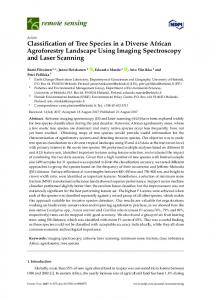
3. Results 3. Results In this study, LST maps for New Brunswick, Canada have been produced using Landsat 5 TM, In this7 study, LSTLandsat maps for Newsensors. Brunswick, Canada have been by produced Landsat 5 TM, Landsat ETM+ and 8 TIRS The LST has been derived using theusing MWA, RTE, Plank Landsat 7 ETM+ and Landsat 8 TIRS sensors. The LST has been derived by using the MWA, RTE, function and the SCA. In the study, Zhang, Wang et al.’s LSE [21] algorithm was considered to be Plank the function and theinSCA. In the study, Zhang, Wang et al.’s LSEresults [21] algorithm was considered to be the most suitable the estimation of LSE as it produced the best in LST extraction. Meteorological most suitable in the estimation of LSE as it produced theLST bestvalues results in LSTfrom extraction. Meteorological data were used to model the accuracy assessment of the derived the sensors. data were used to model the accuracy assessment of the LST values derived from the sensors. Figure 8 shows the LST maps produced by Landsat 5 TM the imagery dated 13 November 2010 Figure showsarea the LST mapsthe produced by Landsat 5 TMMWA the imagery 13 November 2010 from the 8study through use of the SCA, RTE, and thedated Planck function. The from the study area through theinuse the SCA,ofRTE, MWA and meteorological stations used theof modeling the accuracy of the the Planck derivedfunction. LST haveThe alsometeorological been shown on theused maps. stations in the modeling of the accuracy of the derived LST have also been shown on the maps.

(a) Figure 8. Cont.


13 of 31 13 of 33

(b)

(c) Figure 8. Cont.

Remote Sens. 2016, 8, 413 Remote Sens. 2016, 8, 413 Remote Sens. 2016, 8, 413

14 of 31

14 of 33

14 of 33

(d) (d) Figure 8.8. LST LST maps maps derived derived from from Landsat Landsat 5 TM: TM: (a) (a) LSTextracted extracted using the the SCA; (b) (b) LSTextracted extracted Figure Figure 8. LST maps derived from Landsat 55 TM: (a) LST LST extractedusing using theSCA; SCA; (b)LST LST extracted using the the RTE; RTE;(c) (c)LST LSTextracted extractedusing usingthe theMWA; MWA;and and (d)LST LST extractedusing usingthe thePlanck Planckequation. equation. using using the RTE; (c) LST extracted using the MWA; and(d) (d) LSTextracted extracted using the Planck equation.

Figure 9 shows the LST maps produced by the imagery acquired from Landsat 5 TM on 31 Figure 9 shows the LSTmaps maps producedbybythe the imageryacquired acquiredfrom fromLandsat Landsat55TM TMon on31 Figure 92010 shows the December from theLST study area produced through the use of imagery the SCA, RTE, MWA and the Planck function. 31 December 2010 from the study area through the use of the SCA, RTE, MWA and the Planck December 2010 from the studyused areainthrough the useofofthe theaccuracy SCA, RTE, MWA andLST the Planck function. The meteorological stations the modeling of the derived have also been function. The meteorological stations used in the modeling of the accuracy of the LST derived LST have The meteorological stations used in the modeling of the accuracy of the derived have also been shown on the maps. also been shown on the maps. shown on the maps.

(a)

(a) Figure 9. Cont.


15 of 31


15 of 33

(b)

(c)

(d) Figure 9. LST maps derived from Landsat 7 ETM+: (a) LST extracted using the SCA; (b) LST extracted Figure 9. LST maps derived from Landsat 7 ETM+: (a) LST extracted using the SCA; (b) LST extracted using the RTE; (c) LST extracted using the MWA; and (d) LST extracted using the Planck equation. using the RTE; (c) LST extracted using the MWA; and (d) LST extracted using the Planck equation.


16 of 31 16 of 33

Figure 10 shows shows the the LST LSTmaps mapsproduced producedby bythe theimagery imageryacquired acquiredfrom from Landsat 7 ETM+ Landsat 7 ETM+ on on 21 21 November 2010 from study area throughthe theuse useofofthe theSCA, SCA,RTE, RTE,MWA MWAand andthe thePlanck Planckfunction. function. November 2010 from thethe study area through The meteorological stations used in the modeling of the accuracy of the derived LST have also been shown on the maps.

(a)

(b) Figure 10. Cont.


17 of 31 17 of 33

(c)

(d) Figure 10. LST maps derived from Landsat 7 ETM+: (a) LST extracted using the SCA; (b) LST extracted Figure 10. LST maps derived from Landsat 7 ETM+: (a) LST extracted using the SCA; (b) LST extracted using the RTE; (c) LST extracted using the MWA; and (d) LST extracted using the Planck equation. using the RTE; (c) LST extracted using the MWA; and (d) LST extracted using the Planck equation.

Figure 11 shows the LST maps produced by the imagery acquired from Landsat 7 ETM+ on 23 Figure 11 from shows the LST area maps produced by the imagery acquired from 7 ETM+ on February 2016 the study through the use of the SCA, RTE, MWA andLandsat the Planck function. 23 February 2016 from the study area through the use of the SCA, RTE, MWA and the Planck function. The meteorological stations used in the modeling of the accuracy of the derived LST have also been The meteorological shown on the maps.stations used in the modeling of the accuracy of the derived LST have also been shown on the maps.


18 of 31


18 of 33

(a)



19 of 31

19 of 33

(c)

(d) Figure 11.11. LST maps derived usingthe theSCA; SCA;(b) (b)LST LST extracted Figure LST maps derivedfrom fromLandsat Landsat 77 ETM+: ETM+: (a) (a) LST LST extracted extracted using extracted using the RTE; (c) LST extracted using the MWA; and (d) LST extracted using the Planck equation. using the RTE; (c) LST extracted using the MWA; and (d) LST extracted using the Planck equation.

Figure 1212 shows thethe LSTLST maps produced by the imagery acquired from Landsat 8 TIRS on 4 on June Figure shows maps produced by the imagery acquired from Landsat 8 TIRS 2015 from the study area through the use of the SCA, RTE, MWA and the Planck function. The 4 June 2015 from the study area through the use of the SCA, RTE, MWA and the Planck function. meteorological stations used in the in modeling of theof accuracy of theof derived LST have also been shown The meteorological stations used the modeling the accuracy the derived LST have also been onshown the maps. on the maps.


20 of 31


20 of 33

(a)



21 of 31 21 of 33

(c)

(d) Figure 12. LST maps derived from Landsat 8 TIRS: (a) LST extracted using the SCA; (b) LST extracted Figure 12. LST maps derived from Landsat 8 TIRS: (a) LST extracted using the SCA; (b) LST extracted using the RTE; (c) LST extracted using the MWA; and (d) LST extracted using the Planck equation. using the RTE; (c) LST extracted using the MWA; and (d) LST extracted using the Planck equation.

Figure 13 shows the LST maps produced by the imagery acquired from Landsat 8 TIRS on 29 13 shows the area LST through maps produced imagery acquired Landsat 8 TIRSThe on MayFigure 2013 from the study the use ofby thethe SCA, RTE, MWA andfrom the Planck function. 29 May 2013 from the study area through the use of the SCA, RTE, MWA and the Planck function. meteorological stations used in the modeling of the accuracy of the derived LST have also been shown The meteorological stations used in the modeling of the accuracy of the derived LST have also been on the maps. shownThe on accuracy the maps.analysis of the values obtained from the sensors has been done at pixel level by observing the differences between the near surface temperatures obtained from the meteorological


22 of 33

data and the LST stored in a pixel after the use of a land surface temperature extraction algorithm. TablesSens. 6 and show Remote 2016,7 8, 413 the values obtained from the algorithms and the near surface temperatures 22 offor 31 Landsat 5 TM. Tables 8 and 9 show the values obtained from the algorithms and the near surface temperatures for Landsat 7 ETM+. Tables 10 and 11 show the values obtained from the algorithms Thenear accuracy analysis of the values obtained from sensors has are been at pixel level by and the surface temperatures for Landsat 8 TIRS. Allthe temperatures in done degrees Celsius. observing the differences between the near surface temperatures obtained from the meteorological The coordinates of the meteorological stations were converted to shape files and thereafter the data the LST stored in existing a pixel after the pixel use ofthat a land temperature extraction algorithm. land and surface temperature in the the surface meteorological station was located was Tables 6 and 7 show the values obtained from the algorithms and the near surface temperatures for compared to the value of the near surface temperature which was measured by the meteorological Landsat 5 TM. Tables 8 and 9 show the values obtained from the algorithms and the near surface station. In this way, the possible errors were reduced as temperature varies from one place to another temperatures forinLandsat 7 ETM+. 10 andThe 11 locations show the of values obtained from the algorithms and due to changes topography andTables land cover. the meteorological stations have been the near surface temperatures for Landsat 8 TIRS. All temperatures are in degrees Celsius. shown on the maps (Figures 8–13).

(a)



23 of 31


23 of 33

(c)

(d) Figure 13. LST maps derived from Landsat 8 TIRS: (a) LST extracted using the SCA; (b) LST extracted Figure 13. LST maps derived from Landsat 8 TIRS: (a) LST extracted using the SCA; (b) LST extracted using the RTE; (c) LST extracted using the MWA; and (d) LST extracted using the Planck equation. using the RTE; (c) LST extracted using the MWA; and (d) LST extracted using the Planck equation.

The coordinates of the meteorological stations were converted to shape files and thereafter the land surface temperature existing in the pixel that the meteorological station was located was compared to the value of the near surface temperature which was measured by the meteorological station. In this way, the possible errors were reduced as temperature varies from one place to another due to changes in topography and land cover. The locations of the meteorological stations have been shown on the maps (Figures 8–13).


24 of 31

Table 6. Comparison between LST values obtained from Landsat 5 TM using the MWA, Planck equation, RTE, SCA and meteorological data obtained on 31 December 2010. Station Name

Latitude

Longitude

Elevation (Meters)

NST (˝ C) at 12:00

RH (%)

MWA (˝ C)

PLANCK (˝ C)

RTE (˝ C)

SCA (˝ C)

Mechanic Settlement Fundy Park (Alma) Cs Buctouche Cda Cs Nappan Auto Saint John A Parrsboro Gagetown A Gagetown Awos A Summerside Mechanic Settlement Root Mean Square Error (RMSE)

45˝ 411 37.040”N 45˝ 361 00.000”N 46˝ 251 49.006”N 45˝ 451 34.400”N 45˝ 191 05.000”N 45˝ 241 48.000”N 45˝ 501 00.000”N 45˝ 501 20.000”N 46˝ 261 28.000”N 45˝ 411 37.040”N

65˝ 091 54.040”W 64˝ 571 00.000”W 64˝ 461 05.009”W 64˝ 141 29.200”W 65˝ 531 08.050”W 64˝ 201 49.000”W 66˝ 261 00.000”W 66˝ 261 59.000”W 63˝ 501 17.000”W 65˝ 091 54.040”W

403 42.7 35.9 19.8 108.8 30.9 50.6 50.6 12.2 403

´3.1 3.6 ´0.9 ´7.9 ´0.2 2.1 ´2.2 ´1 ´0.9 ´3.1

99 62 78 73 69 68 79 77 78 99

´4.75 ´0.91 ´8.06 ´3.46 ´0.29 ´0.29 ´0.91 ´0.29 ´3.46 ´4.75 2.67

´4.70 ´1.29 ´7.64 ´3.55 ´0.73 ´0.73 ´1.29 ´0.73 ´3.55 ´4.70 2.78

´4.55 ´0.73 ´7.85 ´3.26 ´0.11 ´0.11 ´0.73 ´0.11 ´3.26 ´4.55 2.64

´5.56 ´2.17 ´8.48 ´4.42 ´1.62 ´1.62 ´2.17 ´1.62 ´4.42 ´5.56 3.17

NST

Near Surface Temperature (Day light saving was observed); PLANCK Planck Equation; RTE Radiative Transfer Equation; SCA Single Channel Algorithm; RH Relative Humidity.

Table 7. Comparison between LST values obtained from Landsat 5 TM using the MWA, Planck equation, RTE, SCA and meteorological data obtained on 13 November 2010. Station Name

Latitude

Longitude

Elevation (Meters)

NST (˝ C) at 12:00

RH (%)

MWA (˝ C)

PLANCK (˝ C)

RTE (˝ C)

SCA (˝ C)

Mechanic Settlement Fundy Park (Alma) Cs Buctouche Cda Cs Nappan Auto Saint John A Parrsboro Gagetown A Gagetown Awos A Summerside Root Mean Square Error (RMSE)

45˝ 411 37.040”N 45˝ 361 00.000”N 46˝ 251 49.006”N 45˝ 451 34.400”N 45˝ 191 05.000”N 45˝ 241 48.000”N 45˝ 501 00.000”N 45˝ 501 20.000”N 46˝ 261 28.000”N

65˝ 091 54.040”W 64˝ 571 00.000”W 64˝ 461 05.009”W 64˝ 141 29.200”W 65˝ 531 08.050”W 64˝ 201 49.000”W 66˝ 261 00.000”W 66˝ 261 59.000”W 63˝ 501 17.000”W

403 42.7 35.9 19.8 108.8 30.9 50.6 50.6 12.2

15.4 13.1 12.4 12.1 12.2 13.2 11.6 12.0 13.6

40 53 39 52 41 48 36 36 40

15.15 15.70 12.70 14.17 14.83 14.56 10.11 10.96 12.63 1.64

14.97 15.80 12.58 14.26 14.25 14.57 10.27 10.82 12.55 1.58

15.32 15.73 12.90 14.30 15.14 14.70 10.40 11.30 12.88 1.68

13.28 10.86 10.36 10.36 13.27 10.85 8.37 9.86 10.36 2.33

NST

Near Surface Temperature (Day light saving was observed); PLANCK Planck Equation; RTE Radiative Transfer Equation; SCA Single Channel Algorithm; RH Relative Humidity.


25 of 31

Table 8. Comparison between LST values obtained from Landsat 7 ETM+ using the MWA, Planck equation, RTE, SCA and meteorological data obtained on 21 November 2010. Station Name

Latitude

Longitude

Elevation (Meters)

NST (˝ C) at 12:00

RH (%)

MWA (˝ C)

PLANCK (˝ C)

RTE (˝ C)

SCA (˝ C)

Mechanic Settlement Fundy Park (Alma) Cs Buctouche Cda Cs Nappan Auto Saint John A Parrsboro Gagetown Awos A Summerside Mechanic Settlement Root Mean Square Error (RMSE)

45˝ 411 37.040”N 45˝ 361 00.000”N 46˝ 251 49.006”N 45˝ 451 34.400”N 45˝ 191 05.000”N 45˝ 241 48.000”N 45˝ 501 20.000”N 46˝ 261 28.000”N 45˝ 411 37.040”N

65˝ 091 54.040”W 64˝ 571 00.000”W 64˝ 461 05.009”W 64˝ 141 29.200”W 65˝ 531 08.050”W 64˝ 201 49.000”W 66˝ 261 59.000”W 63˝ 501 17.000”W 65˝ 091 54.040”W

403 42.7 35.9 19.8 108.8 30.9 50.6 12.2 403

´6.8 ´1.9 ´4.4 ´4.4 ´3.6 ´2.6 ´2.9 ´3 ´6.8

78 58 64 70 55 60 55 68 78

´11.75 ´5.50 ´9.62 ´8.23 ´6.18 N/A ´3.51 ´8.23 ´11.75 4.03

´11.52 ´5.53 ´9.48 ´8.14 ´6.18 N/A ´3.62 ´8.14 ´11.52 3.94

´11.43 ´5.21 ´9.31 ´7.92 ´5.88 N/A ´3.22 ´7.92 ´11.43 3.75

´12.34 ´6.39 ´10.31 ´8.98 ´7.03 N/A ´4.49 ´8.98 ´12.34 4.73

NST

Near Surface Temperature (Day light saving was observed); PLANCK Planck Equation; RTE Radiative Transfer Equation; SCA Single Channel Algorithm; RH Relative Humidity; N/A—Data not available as a result of Scan Line Corrector (SLC).

Table 9. Comparison between LST values obtained from Landsat 7 ETM+ using the MWA, Planck equation, RTE, SCA and meteorological data obtained on 23 February 2016. Station Name

Latitude

Longitude

Elevation (Meters)

NST (˝ C) at 12:00

RH (%)

MWA (˝ C)

PLANCK (˝ C)

RTE (˝ C)

SCA (˝ C)

Mechanic Settlement Fundy Park (Alma) Cs Buctouche Cda Cs Nappan Auto Parrsboro Moncton lnternational Airport Gagetown A Summerside Root Mean Square Error (RMSE)

45˝ 411 37.040”N 45˝ 361 00.000”N 46˝ 251 49.006”N 45˝ 451 34.400”N 45˝ 241 48.000”N 46˝ 061 44.000”N 45˝ 501 00.000”N 46˝ 261 28.000”N

65˝ 091 54.040”W 64˝ 571 00.000”W 64˝ 461 05.009”W 64˝ 141 29.200”W 64˝ 201 49.000”W 64˝ 401 43.000”W 66˝ 261 00.000”W 63˝ 501 17.000”W

403 42.7 35.9 19.8 30.9 70.7 50.6 12.2

´8.1 ´6.9 ´8.9 ´7.9 ´5.9 ´8 ´8.4 ´7.3

35 50 45 68 49 44 47 55

´14.46 ´10.17 ´5.40 N/A ´7.41 ´4.08 N/A N/A 3.68

´14.31 ´10.15 ´5.53 N/A ´7.48 ´4.25 N/A N/A 3.58

´14.04 ´9.77 ´5.03 N/A ´7.03 ´3.72 N/A N/A 3.61

´15.12 ´10.98 ´6.39 N/A ´8.33 ´5.12 N/A N/A 3.80

NST

Near Surface Temperature (Day light saving was observed); PLANCK Planck Equation; RTE Radiative Transfer Equation; SCA Single Channel Algorithm; RH Relative Humidity; N/A—Data not available as a result of Scan Line Corrector (SLC).


26 of 31

Table 10. Comparison between LST values obtained from Landsat 8 TIRS using the MWA, Planck equation, RTE, SCA and meteorological data obtained on 4 June 2015.

Station Name

Latitude

Longitude

Elevation (m)

NST (˝ C) at 11:00 am

Mechanic Settlement Fundy Park (Alma) Cs Buctouche Cda Cs Nappan Auto Parrsboro Summerside Moncton International Airport Root Mean Square Error (RMSE)

45˝ 411 37.040”N 45˝ 361 00.000”N 46˝ 251 49.006”N 45˝ 451 34.400”N 45˝ 241 48.000”N 46˝ 261 28.000”N 46˝ 061 44.000”N

65˝ 091 54.040”W 64˝ 571 00.000”W 64˝ 461 05.009”W 64˝ 141 29.200”W 64˝ 201 49.000”W 63˝ 501 17.000”W 64˝ 401 43.000”W

403 42.7 35.9 19.8 30.9 12.2 70.7

13.1 12.4 15.1 15.4 15.9 13.9 16.9

NST

RH (%)

MWA (˝ C)

PLANCK (˝ C)

RTE (˝ C)

SCA (˝ C)

57 56 58 63 42 62 44

9.27 13.42 16.66 14.84 11.70 13.44 17.74 2.30

9.65 13.36 16.14 14.40 12.10 13.55 17.55 2.07

9.43 13.51 16.73 15.01 11.69 13.45 17.84 2.28

8.15 11.33 14.20 13.18 9.17 10.82 14.25 3.65

Near Surface Temperature; PLANCK Planck Equation; RTE Radiative Transfer Equation; SCA Single Channel Algorithm; RH Relative Humidity.

Table 11. Comparison between LST values obtained from Landsat 8 TIRS using the MWA, Planck equation, RTE, SCA and meteorological data obtained on 29 May 2013.

Station Name

Latitude

Longitude

Elevation (Meters)

Mechanic Settlement Fundy Park (Alma) Cs Buctouche Cda Cs Nappan Auto Parrsboro Moncton International Airport Gagetown A Gagetown Awos A Summerside Root Mean Square Error (RMSE)

45˝ 411 37.040”N 45˝ 361 00.000”N 46˝ 251 49.006”N 45˝ 451 34.400”N 45˝ 241 48.000”N 46˝ 061 44.000”N 45˝ 501 00.000”N 45˝ 501 20.000”N 46˝ 261 28.000”N

65˝ 091 54.040”W 64˝ 571 00.000”W 64˝ 461 05.009”W 64˝ 141 29.200”W 64˝ 201 49.000”W 64˝ 401 43.000”W 66˝ 261 00.000”W 66˝ 261 59.000”W 63˝ 501 17.000”W

403 42.7 35.9 19.8 30.9 70.7 50.6 50.6 12.2

NST

NST (˝ C) at 11:00 am

RH (%)

MWA (˝ C)

PLANCK (˝ C)

RTE (˝ C)

SCA (˝ C)

17 18.1 20.1 19.3 16.2 20.2 20 20 16.1

27 38 35 35 49 41 31 31 50

22.24 18.41 23.07 21.66 22.04 29.74 15.36 22.02 20.26 4.83

21.80 18.41 22.28 21.06 21.60 28.78 17.58 21.74 19.67 4.33

23.07 19.31 23.98 22.59 22.88 30.24 16.34 22.79 21.26 5.35

18.85 15.53 20.62 19.29 18.77 23.70 13.32 18.06 18.65 3.06

Near Surface Temperature; PLANCK Planck Equation; RTE Radiative Transfer Equation; SCA Single Channel Algorithm; RH Relative Humidity.


27 of 31

4. Discussion One of the challenges of deriving land surface temperatures from space is doing the accuracy assessment of the results using values which have been measured on the ground. This is because satellite imagery covers a large area (the approximate scene size is 170 km north to south by 183 km east to west for Landsat 5 TM, Landsat 7 ETM+ and Landsat 8 TIRS) and the area varies with topography, and land cover. Not only that but also due to the fact that the spatial resolution of satellite imagery is usually different from the measurements which are made on the ground. Atmospheric conditions of a study area can also seriously hamper the accuracy analysis of data, especially the presence of cloud cover. For this reason, the Landsat imagery that has been used in this study had a cloud cover of less than 10%. After LST obtained from Landsat 5 TM, Landsat 7 ETM+ and Landsat 8 TIRS have been resampled, the spatial resolution of the LST values represents 30 meters on the ground. This poses a challenge as a pixel value is an average of an area with 900 m2 on the ground while the data used for the assessment is just a single point (location of a measurement made on the ground) falling within the pixel being assessed. In this study, among the data used included the ones obtained from the Landsat 7 ETM+ satellite sensor; this sensor has been affected by the presence of the Scan Line Corrector (SLC) as from 31 May 2003. Striped imagery was used in the study as a result of the absence of enough meteorological data of the study area before 2003. Some of the meteorological stations used in the accuracy analysis of the Landsat 7 ETM+ image dated 23 February 2016 were affected by stripes. These stations have been shown in Table 9. The derived LST from the satellite imagery used in this study was compared to meteorological data due to the absence of in situ data during the satellite overpass time. According to studies done by previous researchers [29] there exists a relationship between land surface temperature and near surface temperatures. Land surface temperature can even be used to estimate near surface air temperature [39–41]. Authors in [29] used near surface temperatures in the validation of satellite derived land surface temperatures. Due to these reasons, meteorological data was considered as a tool to model the accuracy of the LST derived from the sensors involved in this study. In this study, the LST values which were obtained from the algorithms produced results which were very close. For Landsat 5 TM, the best results were obtained from the RTE and the Planck function which produced RMSE of 2.64 ˝ C and 1.58 ˝ C, respectively. For Landsat 7 ETM+ LST retrieval, the best results were obtained from the RTE and the Planck function with RMSE of 3.75 ˝ C and 3.58 ˝ C respectively. For Landsat 8 TIRS LST retrieval, the best results were obtained from the Planck function and the SCA with RMSE of 2.07 ˝ C and 3.06 ˝ C respectively. This implies that all the algorithms are suitable for the retrieval of LST from the sensors used in the study. The differences in results may be due to the errors which may arise from the simulation of atmospheric parameters, estimation of LSE as well as errors which may arise from the estimation of atmospheric water vapor. It should also be noted that the temperature values used in the accuracy assessment were near surface temperatures measured from the meteorological stations and not actual temperatures of the ground. These temperatures are measured at a height of up to two meters above the ground. Generally, the LST derived from the algorithms had differences of less than 1 ˝ C between each other. The SCA produced LST which were generally lower in comparison to the other algorithms. The SCA has been found to be less accurate in LST estimation by other authors as a result of being highly dependent in atmospheric [24,42] parameters. The algorithm is also affected by errors that may arise from the estimation of land surface emissivities, which can contribute to an error between 0.2 K and 0.7 K [42]. The atmospheric water vapor used in the SCA was obtained from meteorological data. As a result of the data being obtained from points and thereafter an average value being used for a wide area, this may result to bigger discrepancies between the near surface temperatures and the LST values from space. For future studies, it is important to use atmospheric water vapor values which have been obtained from satellites for LST estimation. Atmospheric water vapor is the most variable component of the atmosphere and varies both horizontally and vertically and it may affect the NDVI


28 of 31

of an area [20]. The atmospheric effects arising from clouds, water vapor and aerosols may reduce the contrast between the visible and near infrared reflections and as a result lead to smaller NDVI values [20] hence affecting the LSE which is derived from NDVI. 5. Conclusions The LST maps in this study have been produced using a QIS plugin which was written using the Python programming language. This has demonstrated how powerful open source tools can be in terms of remote sensing and geographic information systems data processing and analysis. As a result of this study being done through the use of open source tools, it encourages the use of Landsat 5 TM, Landsat 7 ETM+ and Landsat 8 TIRS data in the production of land surface temperature maps, the improvement of algorithms and also provides a platform for debates concerning LST extraction from satellite imagery. This plugin enables users from other disciplines such a hydrology, landscape engineering, urban planning and other related fields to easily extract land surface temperature from visible and near infrared satellite imagery. This plugin also enables users to make use of more than one algorithm of land surface temperature estimation and as a result managing to benefit from possible advantages of them while reducing the possible disadvantages which may arise from the use of a single algorithm in land surface temperature estimation. This study also revealed that the MWA, the SCA, the RTE and the Planck function can all be used in the estimation of LST from Landsat 5 TM, Landsat 7 ETM+ and Landsat 8 TIRS. The availability of meteorological data during the satellite overpass time can, however, play a great role towards determining the algorithm to be used in the estimation of LST. This therefore makes the Planck function easier to use in comparison to the other algorithms as it does not require atmospheric variables during the satellite overpass time. In order to obtain better results in the future, researchers should do accuracy analysis of the LST derived from satellite imagery with actual in situ data collected during the satellite overpass time. It is also important to estimate the atmospheric water vapor from satellites instead of using meteorological data as satellite derived atmospheric water vapor provide better average values over spatially large areas than meteorological data. To perform atmospheric correction of NDVI and emissivity, atmospheric correction algorithms such as 6S [43] and Moderate Resolution Atmospheric Transmission (MODTRAN) [44] may be applied. Acknowledgments: This study was supported by Anadolu University Scientific Research Projects Commission under the grant number 1601F031. We sincerely appreciate the research funding, it was provided by Anadolu University for this article. We express high gratitude to the United States Geological Survey (USGS) for making the Landsat data freely available. We would also like to give our special thanks go to the Government of Canada (Environment Canada) for making the historic meteorological data available for use. This has made this study successful in a great extent. Last but not least, we would like to express our deepest gratitude to the QGIS development team who made it possible for us to make use of the QGIS application programming interface for data processing though the development of the plugin. Author Contributions: Both authors contributed in the design and methodology of the study. The Python Plugin was written by Milton Isaya Ndossi while Ugur Avdan worked on the methodology, accuracy assessment, interpretation of the results and the final version of this contribution. Conflicts of Interest: The authors declare no conflict of interest. The founding sponsors had no role in the design of the study; in the collection, analyses, or interpretation of data; in the writing of the manuscript, and in the decision to publish the results.

Abbreviations The following abbreviations are used in this manuscript: NST RH VNIR TIR LST LSE

Near Surface Temperature Relative Humidity Visible and Near Infrared Thermal Infrared Land Surface Temperature Land Surface Emissivity


SCA MWA RTE RS GIS NDVI TOA EOS USGS UTC GDAL DN K OLI TM ETM+ NASA NCEP

29 of 31

Single Channel Algorithm Mono Window Algorithm Radiative Transfer Equation Remote Sensing Geographic Information Systems Normalized Difference Vegetation Index Top of Atmosphere Earth Observation Satellites United States Geological Survey Coordinated Universal Time Geospatial Data Abstraction Library Digital Numbers Kelvin Operational Land Imager Thematic Mapper Enhanced Thematic Mapper Plus National Aeronautics and Space Administration National Centers for Environmental Prediction

References 1.

2. 3.

4. 5. 6.

7. 8. 9. 10. 11. 12. 13. 14.

15. 16.

Wu, P.; Shen, H.; Zhang, L.; Göttsche, F.-M. Integrated fusion of multi-scale polar-orbiting and geostationary satellite observations for the mapping of high spatial and temporal resolution land surface temperature. Remote Sens. Environ. 2015, 156, 169–181. Li, Z.-L.; Tang, B.-H.; Wu, H.; Ren, H.; Yan, G.; Wan, Z.; Trigo, I.F.; Sobrino, J.A. Satellite-derived land surface temperature: Current status and perspectives. Remote Sens. Environ. 2013, 131, 14–37. [CrossRef] Pandya, M.R.; Shah, D.B.; Trivedi, H.J.; Darji, N.P.; Ramakrishnan, R.; Panigrahy, S.; Parihar, J.S.; Kirankumar, A.S. Retrieval of land surface temperature from the Kalpana-1 VHRR data using a single-channel algorithm and its validation over western India. ISPRS J. Photogramm. Remote Sens. 2014, 94, 160–168. [CrossRef] Jiménez-Muñoz, J.-C.; Sobrino, J.A. Split-window coefficients for land surface temperature retrieval from low-resolution thermal infrared sensors. IEEE Geosci. Remote Sens. Lett. 2008, 5, 806–809. [CrossRef] Jiménez-Muñoz, J.C.; Sobrino, J.A. A single-channel algorithm for land-surface temperature retrieval from aster data. IEEE Geosci. Remote Sens. Lett. 2010, 7, 176–179. [CrossRef] Qin, Z.-H.; Karnieli, A.; Berliner, P. A mono-window algorithm for retrieving land surface temperature from landsat TM data and its application to the Israel-Egypt border region. Int. J. Remote Sens. 2001, 22, 3719–3746. [CrossRef] Team, Q.D. QGIS Python Plugins Repository. Available online: http://plugins.qgis.org/ (accessed on 11 May 2016). USGS. Earth Explorer. Available online: http://earthexplorer.usgs.gov/ (accessed on 5 May 2016). Historical Data. Available online: http://climate.weather.gc.ca/ (accessed on 5 May 2016). USGS. Using the USGS Landsat 8 Product. Available online: http://landsat.usgs.gov/Landsat8_Using_ Product.php (accessed on 9 November 2014). USGS. Landsat 8 (L8) Operational Land Imager (OLI) and Thermal Infrared Sensor (TIRS). Available online: http://landsat.usgs.gov/calibration_notices.php (accessed on 9 February 2016). Barsi, J.A.; Schott, J.R.; Hook, S.J.; Raqueno, N.G.; Markham, B.L.; Radocinski, R.G. Landsat-8 thermal infrared sensor (TIRS) vicarious radiometric calibration. Remote Sens. 2014, 6, 11607–11626. [CrossRef] USGS. Frequently Asked Questions about the Landsat Missions. Available online: http://landsat.usgs.gov/ how_is_radiance_calculated.php (accessed on 24 March 2016). Finn, M.P.; Reed, M.D.; Yamamoto, K.H. A Straight forward Guide for Processing Radiance and Reflectance for eo-1 ALI, Landsat 5 tm, Landsat 7 ETM+, and Aster; Unpublished Report; USGS/Center of Excellence for Geospatial Information Science: Washington, DC, USA, 2012. Kruse, P.W.; McGlauchlin, L.D.; McQuistan, R.B. Elements of Infrared Technology: Generation, Transmission and Detection; Wiley: New York, NY, USA, 1962; Volume 1962. Wang, S.L.L. Chapter 8—Land-surface temperature and thermal infrared emissivity. In Advanced Remote Sensing; Wang, S.L.L., Ed.; Academic Press: Boston, FL, USA, 2012; pp. 235–271.


17. 18.

19.

20.

21. 22. 23. 24.

25. 26.

27. 28. 29. 30. 31.

32. 33. 34. 35. 36. 37. 38. 39.

30 of 31

Tang, B.-H.; Wu, H.; Li, C.; Li, Z.-L. Estimation of broadband surface emissivity from narrowband emissivities. Opt. Express 2011, 19, 185–192. [CrossRef] [PubMed] Wang, F.; Qin, Z.; Song, C.; Tu, L.; Karnieli, A.; Zhao, S. An improved mono-window algorithm for land surface temperature retrieval from landsat 8 thermal infrared sensor data. Remote Sens. 2015, 7, 4268–4289. [CrossRef] Vandegriend, A.; Owe, M.; Vugts, H.; Ramothwa, G. Botswana Water and Surface Energy Balance Research Program. Part 1: Integrated Approach and Field Campaign Results; NASA Goddard Space Flight Center: Greenbelt, MD, USA, 1992. Srivastava, P.K.; Han, D.; Rico-Ramirez, M.A.; Bray, M.; Islam, T.; Gupta, M.; Dai, Q. Estimation of land surface temperature from atmospherically corrected landsat TM image using 6S and NCEP global reanalysis product. Environ. Earth Sci. 2014, 72, 5183–5196. [CrossRef] Zhang, J.; Wang, Y.; Li, Y. A C++ program for retrieving land surface temperature from the data of landsat TM/ETM+ band6. Comput. Geosci. 2006, 32, 1796–1805. [CrossRef] Sobrino, J.; Raissouni, N. Toward remote sensing methods for land cover dynamic monitoring: Application to morocco. Int. J. Remote Sens. 2000, 21, 353–366. [CrossRef] Sobrino, J.; Caselles, V.; Becker, F. Significance of the remotely sensed thermal infrared measurements obtained over a citrus orchard. ISPRS J. Photogramm. Remote Sens. 1990, 44, 343–354. [CrossRef] Yu, X.; Guo, X.; Wu, Z. Land surface temperature retrieval from landsat 8 TIRS—Comparison between radiative transfer equation-based method, split window algorithm and single channel method. Remote Sens. 2014, 6, 9829–9852. [CrossRef] Carlson, T.N.; Ripley, D.A. On the relation between NDVI, fractional vegetation cover, and leaf area index. Remote Sens. Environ. 1997, 62, 241–252. [CrossRef] Barsi, J.; Barker, J.L.; Schott, J.R. An atmospheric correction parameter calculator for a single thermal band earth-sensing instrument. In Proceedings of the 2003 IEEE International Geoscience and Remote Sensing Symposium, Toulouse, France, 21–25 July 2003. Yang, J.; Qiu, J. The empirical expressions of the relation between precipitable water and ground water vapor pressure for some areas in china. Sci. Atmos. Sin. 1996, 20, 620–626. Li, J. Estimating land surface temperature from landsat-5 TM. Remote Sens. Technol. Appl. 2006, 21, 322–326. Liu, L.; Zhang, Y. Urban heat island analysis using the landsat TM data and ASTER data: A case study in Hong Kong. Remote Sens. 2011, 3, 1535–1552. [CrossRef] Artis, D.A.; Carnahan, W.H. Survey of emissivity variability in thermography of urban areas. Remote Sens. Environ. 1982, 12, 313–329. [CrossRef] Sinha, S.; Pandey, P.C.; Sharma, L.K.; Nathawat, M.S.; Kumar, P.; Kanga, S. Remote estimation of land surface temperature for different lulc features of a moist deciduous tropical forest region. In Remote Sensing Applications in Environmental Research; Springer: Berlin, Germany; Heidelberg, Germany, 2014; pp. 57–68. Srivastava, P.; Majumdar, T.; Bhattacharya, A.K. Surface temperature estimation in singhbhum shear zone of India using landsat-7 ETM+ thermal infrared data. Adv. Space Res. 2009, 43, 1563–1574. [CrossRef] Goetz, S.; Halthore, R.; Hall, F.; Markham, B. Surface temperature retrieval in a temperate grassland with multiresolution sensors. J. Geophys. Res. 1995, 100, 25397–25410. [CrossRef] Wukelic, G.; Gibbons, D.; Martucci, L.; Foote, H. Radiometric calibration of landsat thematic mapper thermal band. Remote Sens. Environ. 1989, 28, 339–347. [CrossRef] Schott, J.R.; Volchok, W.J. Thematic mapper thermal infrared calibration. Photogramm. Eng. Remote Sens. 1985, 51, 1351–1357. Weng, Q.; Lu, D.; Schubring, J. Estimation of land surface temperature–vegetation abundance relationship for urban heat island studies. Remote Sens. Environ. 2004, 89, 467–483. [CrossRef] Barsi, J.A.; Schott, J.; Palluconi, F.D.; Helder, D.; Hook, S.; Markham, B.; Chander, G.; O’Donnell, E. Landsat tm and ETM+ thermal band calibration. Can. J. Remote Sens. 2003, 29, 141–153. [CrossRef] Jiménez-Muñoz, J.C.; Sobrino, J.A. A generalized single-channel method for retrieving land surface temperature from remote sensing data. J. Geophys. Res. 2003, 108. [CrossRef] Cresswell, M.; Morse, A.; Thomson, M.; Connor, S. Estimating surface air temperatures, from meteosat land surface temperatures, using an empirical solar zenith angle model. Int. J. Remote Sens. 1999, 20, 1125–1132. [CrossRef]


40. 41. 42. 43.

44.

31 of 31

Prihodko, L.; Goward, S.N. Estimation of air temperature from remotely sensed surface observations. Remote Sens. Environ. 1997, 60, 335–346. [CrossRef] Stisen, S.; Sandholt, I.; Nørgaard, A.; Fensholt, R.; Eklundh, L. Estimation of diurnal air temperature using MSG SEVIRI data in West Africa. Remote Sens. Environ. 2007, 110, 262–274. [CrossRef] Jiménez-Muñoz, J.; Sobrino, J. Error sources on the land surface temperature retrieved from thermal infrared single channel remote sensing data. Int. J. Remote Sens. 2006, 27, 999–1014. [CrossRef] Kotchenova, S.Y.; Vermote, E.F. Validation of a vector version of the 6s radiative transfer code for atmospheric correction of satellite data. Part II. Homogeneous Lambertian and anisotropic surfaces. Appl. Opt. 2007, 46, 4455–4464. [CrossRef] [PubMed] Berk, A.; Bernstein, L.S.; Robertson, D.C. Modtran: A Moderate Resolution Model for Lowtran; DTIC Document: Belvoir, VA, USA, 1987. © 2016 by the authors; licensee MDPI, Basel, Switzerland. This article is an open access article distributed under the terms and conditions of the Creative Commons Attribution (CC-BY) license (http://creativecommons.org/licenses/by/4.0/).