remote sensing

remote sensing Article

Evaluation of an Airborne Remote Sensing Platform Consisting of Two Consumer-Grade Cameras for Crop Identification Jian Zhang 1,2 , Chenghai Yang 2, *, Huaibo Song 2,3 , Wesley Clint Hoffmann 2 , Dongyan Zhang 2,4 and Guozhong Zhang 5 1 2

3 4 5

*

College of Resource and Environment, Huazhong Agricultural University, 1 Shizishan Street, Wuhan 430070, China; [email protected] USDA-Agricultural Research Service, Aerial Application Technology Research Unit, 3103 F & B Road, College Station, TX 77845, USA; [email protected] (H.S.); [email protected] (W.C.H.); [email protected] (D.Z.) College of Mechanical and Electronic Engineering, Northwest A&F University, 22 Xinong Road, Yangling 712100, China Anhui Engineering Laboratory of Agro-Ecological Big Data, Anhui University, 111 Jiulong Road, Hefei 230601, China College of Engineering, Huazhong Agricultural University, 1 Shizishan Street, Wuhan 430070, China; [email protected] Correspondence: [email protected]; Tel.: +1-979-571-5811; Fax: +1-979-260-5169

Academic Editors: Mutlu Ozdogan, Clement Atzberger and Prasad S. Thenkabail Received: 21 January 2016; Accepted: 11 March 2016; Published: 18 March 2016

Abstract: Remote sensing systems based on consumer-grade cameras have been increasingly used in scientific research and remote sensing applications because of their low cost and ease of use. However, the performance of consumer-grade cameras for practical applications has not been well documented in related studies. The objective of this research was to apply three commonly-used classification methods (unsupervised, supervised, and object-based) to three-band imagery with RGB (red, green, and blue bands) and four-band imagery with RGB and near-infrared (NIR) bands to evaluate the performance of a dual-camera imaging system for crop identification. Airborne images were acquired from a cropping area in Texas and mosaicked and georeferenced. The mosaicked imagery was classified using the three classification methods to assess the usefulness of NIR imagery for crop identification and to evaluate performance differences between the object-based and pixel-based methods. Image classification and accuracy assessment showed that the additional NIR band imagery improved crop classification accuracy over the RGB imagery and that the object-based method achieved better results with additional non-spectral image features. The results from this study indicate that the airborne imaging system based on two consumer-grade cameras used in this study can be useful for crop identification and other agricultural applications. Keywords: consumer-grade camera; crop identification; RGB; near-infrared; pixel-based classification; object-based classification

1. Introduction Remote sensing has played a key role in precision agriculture and other agricultural applications [1]. It provides a very efficient and convenient way to capture and analyze agricultural information. As early as 1972, the Multispectral Scanner System (MSS) sensors were used for accurate identification of agricultural crops [2]. Since then, numerous commercial satellite and custom-built airborne imaging systems have been developed for remote sensing applications with agriculture being

Remote Sens. 2016, 8, 257; doi:10.3390/rs8030257

www.mdpi.com/journal/remotesensing

Remote Sens. 2016, 8, 257

2 of 23

one of the major application fields. Remote sensing is very mysterious for most people who usually perceive it as complex designs and sophisticated sensors on satellites and other platforms. This is true for quite a long time, especially for the scientific-grade remote sensing systems on satellites and manned aircraft. However, with the advances of electronic imaging technology, remote sensing sensors have significant breakthroughs, including digitalization, miniaturization, ease of use, high resolution, and affordability. Recently, more and more imaging systems based on consumer-grade cameras have been designed as remote sensing platforms [3–6]. As early as in the 2000s, consumer-grade cameras with 35 mm film were mounted on a unmanned aerial vehicle (UAV) platform to acquire imagery in a small area for range and resource managers [7]. Remote sensing systems with consumer-grade cameras have such advantages over scientific-grade platforms as low cost with high spatial resolution [8,9] and easy deployment [7]. There are two main types of consumer-grade cameras: non-modified and modified. The non-modified cameras capturing visual light with R, G, and B channels have been commonly used since the early periods of consumer-grade cameras for remote sensing [7,10,11]. Additionally, this type of cameras have been commonly used for aerial photogrammetric surveys [12]. However, most scientific-grade remote sensing sensors include near-infrared (NIR) detection capabilities due to its sensitivity for plants, water and other cover types [13]. Therefore, using modified cameras to capture NIR light with different modifying methods is becoming popular. Modified NIR cameras are generally obtained by replacing the NIR-blocking filter in front of the complementary metal-oxide-semiconductor (CMOS) or the charge-coupled device (CCD) with a long-pass NIR filter. A dual-camera imaging system is a common choice with one camera for normal color imaging and the other for NIR imaging [14,15]. With a dual-camera configuration, four-band imagery with RGB and NIR sensitivities can be captured simultaneously. Some consumer-grade cameras have been modified to capture this imagery by this method [10]. The other method is to remove the internal NIR-blocking filter and replace it with a blue-blocking [16] or a red-blocking filter [17]. This method can capture three-band imagery, including the NIR band and two visible bands, with just one single camera. Both methods can be implemented, but both still have some issues [16]. The separate RGB and NIR images from dual cameras need to be registered for dual cameras. The NIR light may influence the other two bands for the single camera when capturing the NIR band. In other words, extensive post-processing is required to get the desired imagery. Therefore, it is necessary to decide if a simple unmodified RGB camera or a relatively complex dual-camera system with the NIR band should be selected. Many remote sensing imaging systems based on unmodified single cameras have been used for some agricultural applications to achieve satisfying results [9,14,18]. Consumer-grade cameras cannot capture very detail spectral information, but most of them can obtain very high or ultra-high ground resolution because these cameras can be carried on such low-flying platforms as UAV, airplanes and balloons. Moreover, with the rapid advancement of object-based image analysis (OBIA) methods, imagery with abundant shape, texture and context information could usually improve classification performance for practical applications [19,20]. Therefore, to choose pixel-based or object-based image processing methods is another question that needs to be considered. Despite some shortcomings, consumer-grade cameras with the attributes of low cost and easy deployment have been gradually used in different application fields in the last decade, in particular for agricultural applications, such as crop identification [10], monitoring [11,14,21], mapping [9], pest detection [18], species invasion [17] and crop phenotyping [6,22]. It is becoming a reality for farmers to use these consumer-grade cameras for crop production and protection. Therefore, it is important to evaluate and compare the performances of normal RGB cameras and modified NIR cameras using different image processing methods. Scientists at the Aerial Application Technology Research Unit at the U.S. Department of Agriculture-Agricultural Research Service’s Southern Plains Agricultural Research Center in College Station, Texas has assembled a dual-camera imaging system with both visible and NIR sensitivities


3 of 23

using two consumer-grade cameras. The overall goal of the study was to evaluate the performance of RGB imagery alone and RGB combined with NIR imagery for crop identification. The specific Remotewere Sens. 2016, 8, 257 24 objectives to: (1) compare the differences between the three-band imagery and four-band3 of imagery for crop identification; (2) assess the performance on image classification between the object-based and imagery for crop identification; (2) assess the performance on image classification between the objectpixel-based analysis methods; and (3) make recommendations for the selection of imaging systems based and pixel-based analysis methods; and (3) make recommendations for the selection of imaging and imagery processing methods for practical applications. systems and imagery processing methods for practical applications.

2. Materials and Methods

2. Materials and Methods

2.1. Study Area

2.1. Study Area

This This study waswas conducted at at the Valley near nearCollege College Station, Texas, in July study conducted theBrazos BrazosRiver River Valley Station, Texas, in July 2015 2015 2 2 (Figure withinwithin a cropping areaarea of 21.5 kmkm(Figure 1). islocated locatedatatthe the lower part of the Brazos a cropping of 21.5 1).This This area area is lower part of the Brazos RiverRiver (the “Brazos Bottom”) with humid subtropical (the “Brazos Bottom”) with humid subtropicalclimate. climate.

Figure 1. The study area: (a) Geographic map of the study area, which is located in the bottom of

Figure 1. The study area: (a) Geographic map of the study area, which is located in the bottom of Brazos basin and near College Station, Texas; and (b) image map of the study area from Google Earth. Brazos basin and near College Station, Texas; and (b) image map of the study area from Google Earth.

In this area, the main crops were cotton, corn, sorghum, soybean and watermelon in the 2015

In this area, the main crops were cotton, corn, sorghum, soybean and watermelon in the 2015 growing season. Cotton was the main crop with the largest cultivated area, and it had very diverse growing season. Cottondue wastothe main crop withdates the largest cultivatedconditions. area, and it hadcornfields very diverse growing conditions different planting and management Most growing conditions due to different planting dates and management conditions. Most were near physiological maturity with very few green leaves, and most of sorghum fields were cornfields in the were generative near physiological maturity with verysenescence few greenatleaves, and most of sorghum fields phase reflected by beginning the imaging time. Especially corn was were dryingin the generative phase reflected by beginning senescence at at thethe imaging time. Especially drying in in fields for harvest. Soybean and watermelon were vegetative growth stages.corn Due was to cloudy weather in much May and June, aerial imagery was not acquired during theto optimum fieldsand for rainy harvest. Soybean andofwatermelon were at the vegetative growth stages. Due cloudy and of crop discrimination, based onaerial the crop calendars this study area. However, this type period of rainy period weather in much of May and June, imagery wasfor not acquired during the optimum weather conditions is probably a common dilemma for agricultural remote sensing. of crop discrimination, based on the crop calendars for this study area. However, this type of weather conditions is probably a common dilemma for agricultural remote sensing. 2.2. Imaging System and Airborne Image Acquisition

2.2. Imaging System and Airborne Image Acquisition 2.2.1. Imaging System and Platform

The dual-camera imaging system used in this study consisted primarily of two Nikon D90 digital 2.2.1. Imaging System and Platform CMOS cameras with Nikon AF Nikkor 24mm f/2.8D lenses (Nikon, Inc., Melville, NY, USA). One

The dual-camera system used in this The study consisted primarily Nikon camera was used to imaging capture three-band RGB images. other camera was modifiedoftotwo capture NIR D90 digital CMOS cameras with Nikon AF Nikkor 24mm f/2.8D lenses (Nikon, Inc., Melville, NY, images after the infrared-blocking filter installed in front of the CMOS of the camera was replaced byUSA). One camera was used tofilter capture RGBMukilteo, images. WA, The other was modified to a 720 nm long-pass (Lifethree-band Pixel Infrared, USA). camera The other components of capture the NIR images after the two infrared-blocking in front of theremote CMOStrigger of theascamera replaced system included GPS receivers, afilter videoinstalled monitor and a wireless shown was in Figure 2. The description of this system can be Mukilteo, found in a single-camera imaging described by a 720 nmdetailed long-pass filter (Life Pixel Infrared, WA, USA). The othersystem components of the by Yang et al. [18]. The difference between the two imaging systems was that the single-camera system included two GPS receivers, a video monitor and a wireless remote trigger as shown in Figure 2. system contained onlyofone D90can camera for taking images, while the dual-camera system by The detailed description thisNikon system be found in a RGB single-camera imaging system described had a the RGB camera and a modified camera for NIR imaging necessary for this study. This dualYang et al. [18]. The difference between the two imaging systems was that the single-camera system camera imaging system was attached via a camera mount box on to an Air Tractor AT-402B as shown contained only one Nikon D90 camera for taking RGB images, while the dual-camera system had a the in Figure 2.


4 of 23

RGB camera and a modified camera for NIR imaging necessary for this study. This dual-camera imaging system wasSens. attached via a camera mount box on to an Air Tractor AT-402B as shown in Figure42.of 24 Remote 2016, 8, 257

Figure 2. Imaging system and platform: (a) Components of the imaging system (two Nikon D90

Figure 2. Imaging system and platform: (a) Components of the imaging system (two Nikon D90 cameras with Nikkor 24 mm lenses, two Nikon GP-1A GPS receiver, a 7-inch portable LCD video cameras with Nikkor 24 mm lenses, two Nikon GP-1A GPS receiver, a 7-inch portable LCD video monitor, a wireless remote shutter release); (b) cameras mounted on the right step of an Air Tractor monitor, a wireless remote shutter release); (b) cameras camera mounted the(d) right step picture of an Air Tractor AT-402B; (c) close-up picture showing the custom-made box;on and close-up of the AT-402B; (c) close-up picture showing the custom-made camera box; and (d) close-up picture of the cameras in the box. cameras in the box. 2.2.2. Spectral Characteristics of the Cameras

2.2.2. Spectral Characteristics of the Cameras The spectral sensitivity of the two cameras was measured in the laboratory through a monochromator (Optical Building Edison, NJ, measured USA) and a in calibrated photodiode. The The spectral sensitivity of theBlocks, two Inc., cameras was the laboratory through a two cameras were spectrally calibrated with the lenses by taking photographs of monochromatic monochromator (Optical Building Blocks, Inc., Edison, NJ, USA) and a calibrated photodiode. The two light from the monochromator projected onto a white panel. A calibrated photodiode was positioned cameras were spectrally calibrated with the lenses by taking photographs of monochromatic light from at the same distance of the camera to measure the light intensity. The relative spectral response of the monochromator projected onto a white panel. A calibrated photodiode was positioned at the same one channel could be calculated for a given wavelength λ and a given channel (RGB) as shown in distance of the(1)camera Equation [23]. to measure the light intensity. The relative spectral response of one channel could be calculated for a given wavelength λ and a given channel (RGB) as shown in Equation (1) [23]. ( , ) ( , )=

( )

,

= , , ;

= 400 − 1000

(1)

C pλ, nq ´ C nq “ response ofdark , n “ r,=g, b; ´ 1000 nm ( ) is the light R pλ, ( , ) is the spectral channel , ,λ “at400 wavelength. I pλq

(1) where intensity measured with the photodiode at wavelength. C(λ, n) is the digital count corresponding mean digital count of theI dark of = ,spectral , at response wavelength. wheretoRchannel pλ, nq is the of channelisnthe “ r, g, b at λ wavelength. pλq isbackground the light intensity channel = , , at wavelength. Wavelength ranged from 400 to 1000 nm, and the measurement measured with the photodiode at λ wavelength. C(λ, n) is the digital count corresponding to channel wavelength interval was 20 nm. The average digital count for each channel was determined for the n “ r, g, b at λ wavelength. Cdark is the mean digital count of the dark background of channel n “ r, g, b center of the projected light beam using image-processing software (MATLAB R2015a, MathWorks, at λ wavelength. Wavelength ranged from 400 towere 1000recorded nm, andby the wavelength interval Inc., Natick, MA, USA). In addition, the images themeasurement raw camera format. was 20 nm. The average digital count for each channel was determined for the center of thevaried projected From the normalized spectral sensitivity of the two cameras (Figure 3), the sensitivity light from beam400 using image-processing software (MATLAB R2015a, Inc., Natick,camera. MA, USA). to 700 nm for the non-modified camera and from 680 toMathWorks, 1000 nm for the modified With thethe 720images nm long-pass filter, the spectral response roseformat. from 0 at 680 nm to maximum at 720 nm. In addition, were recorded by the raw camera It can be that the spectral sensitivity curves have some overlaps among3), thethe channels of each From theseen normalized spectral sensitivity of the two cameras (Figure sensitivity varied camera. This is very common in consumer-grade cameras, and is also one of the reasons that this from 400 to 700 nm for the non-modified camera and from 680 to 1000 nm for the modifiedtype camera. cameras had not been filter, commonly used for response most scientific in the For the modified With of the 720 nm long-pass the spectral roseapplications from 0 at 680 nmpast. to maximum at 720 nm. camera, the red channel had a much stronger response than the other two channels (blue and green) It can be seen that the spectral sensitivity curves have some overlaps among the channels of each and the monochrome imaging mode in the NIR range. Thus, the red channel was chosen as the NIR camera. This is very common in consumer-grade cameras, and is also one of the reasons that this type image for remote sensing applications. of cameras had not been commonly used for most scientific applications in the past. For the modified camera, the red channel had a much stronger response than the other two channels (blue and green)


5 of 23

and the monochrome imaging mode in the NIR range. Thus, the red channel was chosen as the NIR image for remote sensing applications. Remote Sens. 2016, 8, 257

5 of 24

Figure 3. Normalized spectral sensitivity of two Nikon D90 cameras and relative reflectance of 10

Figure 3.land Normalized spectral sensitivity of two Nikonlines D90represent camerasdifferent and relative reflectance of 10 land use and land cover (LULC) classes. The dotted channels of the RGB use and camera land cover (LULC)Nikon-color-g, classes. Theand dotted lines represent channels the RGB camera (Nikon-color-r, Nikon-color-b) and the different modified NIR camera of (Nikon-nir-r, Nikon-nir-g, Nikon-nir-b,and andNikon-color-b) Nikon-nir-mono). The solid lines represent the relative reflectance of (Nikon-color-r, Nikon-color-g, and the modified NIR camera (Nikon-nir-r, Nikon-nir-g, 10 LULC Nikon-nir-b, andclasses. Nikon-nir-mono). The solid lines represent the relative reflectance of 10 LULC classes. 2.3. Image Acquisition and Pre-Processing

2.3. Image Acquisition and Pre-Processing 2.3.1. Airborne Image Acquisition

2.3.1. Airborne Image Acquisition

Airborne images were taken from the study area at altitudes of 1524 m (5000 ft.) above ground

Airborne images taken from the study ofunder 1524 sunny m (5000 ft.) above level (AGL) with were a ground speed of 225 km/h (140area mph)at onaltitudes 15 July 2015 conditions. The ground spatialwith resolution was 0.35 m at order to achieve least2015 50% overlaps along and level (AGL) a ground speed ofthis 225height. km/hIn(140 mph) on 15atJuly under sunny conditions. between the flight lines, images acquired In at 5-s intervals. Both cameras The spatial resolution was 0.35 m atwere this height. order to achieve at leastsimultaneously 50% overlapsand along and independently captured 144 images each over the study. Moreover, each image was recorded in both between the flight lines, images were acquired at 5-s intervals. Both cameras simultaneously and 12-bit RAW format for processing and JPG format for viewing and checking. independently captured 144 images each over the study. Moreover, each image was recorded in both 2.3.2.format Image Pre-Processing 12-bit RAW for processing and JPG format for viewing and checking. Vignetting and geometric distortion problems are the inherent issues of most cameras which

2.3.2. Image Pre-Processing usually cause some inaccuracy in image analysis results, especially for modified cameras [21,24]. Therefore,and the free Capture NX-D 1.2.1 software (Nikon, Japan)issues provided thecameras camera which Vignetting geometric distortion problems areInc., theTokyo, inherent of with most manufacturer was used to correct the vignetting and geometric distortion in the images. The usually cause some inaccuracy in image analysis results, especially for modified cameras [21,24]. corrected images were saved in 16-bit TIFF format to preserve image quality. Therefore, the freewere Capture NX-Dto1.2.1 softwarefor (Nikon, Inc., Tokyo, Japan) provided with the camera There 144 images be mosaicked each camera. The Pix4D Mapper software (Pix4D, manufacturer was used to correct the vignetting and geometric distortion in the images. The corrected Inc., Lausanne, Switzerland) was selected, which is a software package for automatic image mosaicking with high accuracy [25]. To improve the positional accuracy of the mosaicked image, images were saved in 16-bit TIFF format to preserve image quality. some white plastic square with a sidefor of each 1 m were placedThe across the study area. A Trimble GPS There were 144 images to panels be mosaicked camera. Pix4D Mapper software (Pix4D, Inc., Pathfinder ProXRT receiver (Trimble Navigation Limited, Sunnyvale, CA, USA), which provided a Lausanne, Switzerland) was selected, which is a software package for automatic image mosaicking 0.2-m average horizontal position accuracy with the real-time OmniSTAR satellite correction, was with high accuracy To improve positional accuracy the mosaicked some used to collect [25]. the coordinates fromthe these panels. Fifteen groundofcontrol points (GCP)image, as shown in white plastic square panels with a side of 1 m were placed across the study area. A Trimble GPS Pathfinder Figure 1 were used for geo-referencing. As shown in Figure 4, the spatial resolutions were 0.399 and m for(Trimble the mosaicked RGB andLimited, NIR images. The absolute horizontal positionprovided accuracy was 0.470 average ProXRT 0.394 receiver Navigation Sunnyvale, CA, USA), which a 0.2-m and 0.701 m for the respective mosaicked images. These positional errors were well within 1 to to 3 collect horizontal position accuracy with the real-time OmniSTAR satellite correction, was used times of the ground sampling distance (GSD) or spatial resolution [26]. the coordinates from these panels. Fifteen ground control points (GCP) as shown in Figure 1 were used for geo-referencing. As shown in Figure 4, the spatial resolutions were 0.399 and 0.394 m for the mosaicked RGB and NIR images. The absolute horizontal position accuracy was 0.470 and 0.701 m for the respective mosaicked images. These positional errors were well within 1 to 3 times of the ground sampling distance (GSD) or spatial resolution [26].

Remote Sens. 2016, 8, 257 Remote Sens. 2016, 8, 257

6 of 23 6 of 24

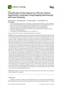
Figure 4. Mosaicked images forforthis band 11 ==blue, blue,band band2 2= =green green Figure 4. Mosaicked images thisstudy: study:(a) (a)three-band three-band RGB RGB image, band band = red; NIR bandimage; image;and and(c) (c)CIR CIR composite composite (NIR, andand band 3 =3red; (b)(b) NIR band (NIR, red redand andgreen) green)extracted extractedfrom fromthe the four-band image, band 1 = blue, band 2 = green, band 3 = red and band 4 = NIR. four-band image, band 1 = blue, band 2 = green, band 3 = and band 4 = NIR.


7 of 23

To generate a mosaicked four-band image, the mosaicked RGB and NIR images were registered to each other using the AutoSync module in ERDAS Imagine (Intergraph Corporation, Madison, AL, USA). The RGB image was chosen as the reference image as it had better image quality than the NIR image. Several tie control points were chosen manually before the automatic registration. Thousands of tie points were generated by AutoSync and a third-order polynomial geometric model as recommended with the number of tie points was used [27]. The root mean square (RMS) error for the registration was 0.49 pixels or 0.2 m. The combined image was resampled to 0.4-m spatial resolution. The color-infrared (CIR) composite of the four-band image is shown in Figure 4. 2.4. Crop Identification Selection of different band combinations and classification methods generally influence classification results. To quantify and analyze these effects on crop identification results, three typical and general image classification methods (unsupervised, supervised and object-based) were selected. Meanwhile, to examine how numbers of LULC classes affect the classification results, six different class groupings were defined as shown in Table 1. It should be noted that the three-band or four-band image was first classified into 10 classes and then the classification results were regrouped into six, five, four, three and two classes. For the ten-class grouping, the impervious class mainly included solid roads and buildings. Bare soil and fallow were grouped in one class and the water class included river, ponds, and pools. Considering soybeans and watermelon accounted for only a small portion of the study area, they were treated as non-crop vegetation with grass and forest in the five-class grouping and as non-crop in the four- and three-class groupings. Table 1. Definition of six different class groupings for image classification. Table 1. Definition of six different class groupings for image classification. Ten-Class impervious bare soil and fallow water grass forest soybean watermelon corn sorghum cotton

Six-Class

non-crop

soybean watermelon corn sorghum cotton

Five-Class non-crop (non-vegetation)

non-crop (vegetation) corn sorghum cotton

Four-Class

Three-class

non-crop non-crop (with soybean and (with soybean watermelon) and watermelon)

corn sorghum cotton

grain

Two-Class

non-crop

crop

cotton

2.4.1. Pixel-Based Classification The unsupervised Iterative Self-Organizing Data (ISODATA) and the supervised maximum likelihood classification were chosen as pixel-based methods in this study. Given the diversity and complexity of the land cover in the study area, the number of clusters was set to ten times of the number of land cover classes. The number of maximum interactions was set to 20 and the convergence threshold to 0.95. Then all of the clusters were assigned to the 10 land cover classes. For the supervised maximum likelihood classification, each class was further divided into 3 to 10 subclasses due to the variability within each of the land cover classes. After supervised classification, these subclasses were merged. For each subclass, 5 to 15 training samples were selected and the total number of training samples was almost equal to the number of clusters in ISODATA. The same training samples were used for supervised classification for both the three-band and four-band images. 2.4.2. Object-Based Classification OBIA has been recognized to have outstanding classification performance for high-resolution imagery. Segmentation and definition of classification rules are the main steps of object-based


8 of 24

2.4.2. Object-Based Classification Remote Sens. 2016, 8, 257

8 of 23

OBIA has been recognized to have outstanding classification performance for high-resolution imagery. Segmentation and definition of classification rules are the main steps of object-based classification. In In order order to toshow showaatransparent transparentprocess processand andobtain obtainananobjective objective result, estimation result, thethe estimation of of scale parameter (ESP) tool was used for chosing segmentation parameters [28] and the classifier scale parameter (ESP) tool was used for chosing segmentation parameters [28] and known as classification classification and and regression regression tree tree(CART) (CART)was wasused usedfor forgenerating generatingclassification classificationrules. rules. Segmentation for object-based classification was performed using the commercial commercial software software eCognition Developer (Trimble Inc., Munich, Germany). The segmentation processing that integrates eCognition Developer (Trimble Inc., Munich, Germany). processing spectral, shape and compactness factors is very important for the subsequent subsequent classification [29], but standardized or widely accepted methods are lacking to determine the optimal scale for different types types of imagery imagery or applications applications [30]. To minimize minimize the influence influence of of contrived contrived factors factors in in this step, some reference segmentation scales can be estimated by the estimation of scale parameter (ESP) tool [28], which which evaluates evaluates variation variation in in heterogeneity heterogeneity of of image image objects objects that that are are iteratively iteratively generated generated at multiple scale appropriate scales. ForFor thisthis study, a scale step step of 50of was to set findtosome scale levels levelsto toobtain obtainthe themost most appropriate scales. study, a scale 50 set was find optimal segmentation scales from 0 to 10,000 with the ESP parameters some optimal segmentation scales from 0 to 10,000 withtool, the and ESPthree tool,segmentation and three segmentation (SP) (1900, 4550 9200) had been estimated. simplify the SP 4550 was for parameters (SP)and (1900, 4550 and 9200) had beenToestimated. To processing, simplify thethe processing, theused SP 4550 image segmentation, which is suitable for most of landfor cover without or was used for image segmentation, which is suitable mostclasses of land cover over-segmentation classes without overunder-segmentation. To further improve the segmentation results, spectral difference segmentation segmentation or under-segmentation. To further improve the segmentation results, spectral with a scalesegmentation of 1000 was performed to merge objects similar spectral objects values. with The difference with a scale of 1000neighboring was performed to with merge neighboring three-band and four-band image segmentation producedimage 970 and 950 image objects, respectively, as similar spectral values. The three-band and four-band segmentation produced 970 and 950 shown in Figure 5. image objects, respectively, as shown in Figure 5.

Figure 5. 5. Image results: (a) (a) three-band image segmentation segmentation with with 970 970 image image objects; objects; and and Figure Image segmentation segmentation results: three-band image (b) four-band image segmentation with 950 image objects. (b) four-band image segmentation with 950 image objects.

The classification pattern of object-based classification like eCongnition is mainly based on a The classification pattern of object-based classification like eCongnition is mainly based on a series of rules from several features. User knowledge and past experience could be transferred to series of rules from several features. User knowledge and past experience could be transferred to some constraint rules for classification [31]. However, it is very unreliable and highly individualized. some constraint rules for classification [31]. However, it is very unreliable and highly individualized. Therefore, the CART algorithm was used for the training of object-based classification rules [32]. Therefore, the CART algorithm was used for the training of object-based classification rules [32]. Because it is a non-parametric rule-based classifier and has a “white box” workflow [30], the structure Because it is a non-parametric rule-based classifier and has a “white box” workflow [30], the structure and terminal nodes of a decision tree is easy to interpret, allowing the user to know the mechanism and terminal nodes of a decision tree is easy to interpret, allowing the user to know the mechanism of of the object-based classification method and evaluate it. the object-based classification method and evaluate it. The CART classifier included in eCongnition could create the decision-tree model based on some The CART classifier included in eCongnition could create the decision-tree model based on some features from training samples. In order to minimize the impact by the selection of different sample features from training samples. In order to minimize the impact by the selection of different sample sets, the sample sets used in the supervised classification was also used. The difference was that the samples sets, the sample sets used in the supervised classification was also used. The difference was that the were turned into image objects. Then these image objects containing the class information were used samples were turned into image objects. Then these image objects containing the class information as the training samples for the object-based classification. There were three main feature types used were used as the training samples for the object-based classification. There were three main feature


9 of 23

types used for modeling: layer spectral features including some vegetation indices (VIs), shape features, and texture features (Table 2) [33–45]. Table 2. List of object features for decision tree modeling. Source

Feature Types

(1) 1 Normalized Difference Vegetation index (NDVI) = (NIR ´ R)/(NIR + R) [33] (2) Ratio Vegetation index (RVI) = NIR/R [34] (3) Difference Vegetation index (DVI) = NIR ´ R [35] ? (4) Renormalized Difference Vegetation Index(RDVI) = NDVI ˆ DVI [36] (5) NDWI = (G ´ NIR)/(G + NIR) [37] (6) Optimization of Soil-adjusted Vegetation Index (OSAVI) = pNIR ´ Rq { pNIR ` R ` 0.16q [38] (7) Soil Adjusted Vegetation Index c´(SAVI) = 1.5¯ˆ pNIR ´ Rq { pNIR ` R ` 0.5q [39] (8) Soil Brightness Index (SBI) = NIR2 ` R2 [40]

VI

References

For Three-Band

Feature Name

ˆ ˆ ˆ ˆ ˆ ˆ

eCognition Geometry Texture

‘

ˆ

‘

ˆ

‘

‘

‘

‘ ‘

‘ ‘

Mean of (17) B,(18) G,(19) R and (20) Brightness Mean of (21) NIR Standard deviation of (22) B,(23) G,(24) R (25) Standard deviation of NIR HIS((26) Hue, (27) Saturation, (28) Intensity)

‘ ‘ ‘ ‘ ‘

‘ ‘ ‘ ‘ ‘

(29) Area, (30) Border length (31) Asymmetry, (32) Compactness, (33) Density, (34) Shape index

‘ ‘

‘ ‘

GLMC ((35) Homogeneity, (36) Contract, (37) Dissimilarity, (38) Entropy, (39) Ang.2nd moment, (40) Mean, (41) StdDev, (42) Correlation)

‘

‘

32

42

(9) B* = B/(B + G + R), (10) G* = G/(B + G + R), (11) R* = R/(B + G + R) (12) Excess Green (ExG) = 2G* ´ R* ´ B* [41], (13) Excess Red (ExR) = 1.4R* ´ G* [42], (14) ExG ´ ExR [43] (15) CIVE = 0.441R ´ 0.811G + 0.385B + 18.78745 [44] (16) Normalized Difference index (NDI) = (G ´ R)/(G + R) [45]

Layer

For Four-Band ‘ ‘ ‘ ‘ ‘

Total Number of Features 1

(n) is the number for each feature, ranging from (1) to (42).

2.5. Accuracy Assessment For accuracy assessment, 200 random points were generated and assigned to each class in a stratified random pattern based on each classification map. At least 10 points were generated for each class. For this study, three classification methods were applied to two types of images, so there were six classification maps. A total of 1200 points were used for accuracy assessment of the six classification maps [30]. The number of points and percentages by class type are given in Table 3. Ground verification of all the points for the LULC classes was performed shortly after image acquisition for this study area. If one or more points fell within a field, the field was checked. Overall accuracy [46], confusion matrix [47], and kappa coefficient [48] were calculated. In order to evaluate the performance of the image types and methods, average kappa coefficients were calculated by class and by method. Table 3. Count and percentage by class type for 1200 reference points. Class Type

Count

Percentage

Class Type

Count

Percentage

Impervious Bare Soil and Fallow Grass Forest Water

55 186 162 106 69

4.6% 15.6% 13.5% 8.8% 5.8%

Soybean Watermelon Corn Sorghum Cotton

29 49 100 115 329

2.4% 4.1% 8.3% 9.6% 27.3%

3. Results 3.1. Classification Results Figure 6 shows the ten-class classification maps based on the three methods applied to the three-band and four-band images, including unsupervised classification for the three-band image (3US), unsupervised classification for the four-band image (4US), supervised classification for the three-band image (3S), supervised classification for the four-band image (4S), object-based classification


10 of 23

for the three-band image (3OB), and object-based classification for the four-band image (4OB). To compare the actual differences between the pixel-based and object-based methods directly [29], no such post-processing operations as clump, sieve, and eliminate were perfomed for the pixel-based classification maps and no generalization was applied to the object-based classification maps either. Remote Sens. 2016, 8, 257 11 of 24

Figure 6. Image classificationresults results (ten-class): (a) unsupervised classification for three-band Figure 6. Image classification (ten-class): (a) unsupervised classification forimage three-band (3US); (b) unsupervised classification for four-band image (4US), (c) supervised classification for threeimage (3US); (b) unsupervised classification for four-band image (4US), (c) supervised classification band image (3S); (d) supervised classification for four-band image (4S); (e) object-based classification for for three-band image (3S); (d) supervised classification for four-band image (4S); (e) object-based three-band image (3OB); and (f) object-based classification for three-band image (4OB). classification for three-band image (3OB); and (f) object-based classification for three-band image (4OB).


11 of 23

Most of the classification maps appear to distinguish different land cover types reasonably well. From a visual perspective, the “salt-and-pepper” effect on the pixel-based maps is the obvious difference with the object-based maps. The object-based maps present a very good visual effect as different cover types are shown by the homogenous image objects. Without considering the accuracy of the maps, the object-based classification maps look cleaner and more appropriate to produce thematic maps. Visually, it is difficult to evaluate the differences between the unsupervised and supervised methods or between the three-band and four-band images. Specifically, the classification results of water and impervious had high consistence. Because of the lack of NIR band, some water areas in the three-band image was classified as bare soil and fallow for all the methods. Sorghum and corn were difficult to distinguish because both crops were at their late growth stages with reduced green leaf area. Corn was close to physiological maturity and above ground biomass was fully senescent, whereas sorghum was in the generative phase and started senescence, but still had significant green leaf material. Although late growth stages casued a reduction in canopy NDVI values for both corn and sorghum, the background weeds and soil exposure also affected the overall NDVI values. All crops and cover types show varying degrees of confusion among themselves. This problem also occurred in the object-based maps, but it does not appear to be as obvious as in the pixel-based maps. 3.2. Accuracy Assessment Table 4 summarizes the accuracy assessment results for the ten-class and two-class classification maps for the three methods applied to the two images. The accuracy assessment results for the other groupings are discussed and compared with the ten-class and two-class results in Section 4.3. Overall accuracy for the ten-class classification maps ranged from 58% for 3US to 78% for 4OB and overall kappa from 0.51 for 3US to 0.74 for 4OB. As expected, the overall accuracy and kappa were higher for the four-band image than for the three-band image for all the three methods. Among the three methods, the object-based method performed better than the two pixel-based methods, and the supervised method was slightly better than the unsupervised method. For the individual classes, the non-plant classes such as water, impervious, and bare soil and fallow had better and stable accuracy results for all the six scenarios with an average kappa of 0.85, 0.82 and 0.74, respectively. Due to variable growing stages and management conditions, the main crop class cotton had a relatively low accuracy with an average kappa of 0.47 for all the scenarios. Although at later growing stages, sorghum and corn had a relatively good accuracy with an average kappa of 0.67 and 0.62, respectively. The main reason was that both crops were at senescence and had less green leaf material, so they could easily be distinguished with other vegetation. Soybean and watermelon had unstable accuracy results among the six scenarios, but their differentiation was significantly improved with the object-based method. The grass and forest in the study area were difficult to distinguish using the pixel-based methods, but they were more accurately separated with the object-based method. For the two broad classes (crop and non-crop), overall accuracy ranged from 76% for 3US to 91% for 4OB and overall kappa from 0.51 for 3US to 0.82 for 4OB. Clearly, overall accuracy and kappa were generally higher for the two-class maps than for the ten-class maps. The two-class classification maps will be useful for some appliccations when total cropping area information is needed.


12 of 23

Table 4. (a–f) Accuracy assessment results. (a) Unsupervised Classification for Three-Band Image (3US) Ten-class 2 CD 4

Non-crop

crop

IM BF GA FE WA SB WM CO SG CT

RD

Two-class

3

Pa

5

Ua

6

IM

BF

GA

FE

WA

SB

WM

CO

SG

CT

%

%

1

11 143 2 0 9 0 0 16 2 3

0 12 71 1 0 0 14 7 35 22

0 1 7 57 0 0 9 0 4 28

0 3 1 1 61 0 0 2 0 1

0 0 0 24 0 0 0 1 2 2

0 5 9 0 1 0 9 6 17 2

0 13 0 0 0 0 0 72 13 2

0 7 9 0 0 0 0 15 79 5

0 49 17 13 1 0 0 29 62 158

80 77 44 54 88 0 18 72 69 48

80 59 61 59 85 NaN 28 49 37 70

44 9 0 0 0 0 0 0 0 2

Kp 7 0.79 0.71 0.38 0.50 0.88 0.0 0.16 0.68 0.62 0.36

Overall kappa=0.51 Overall accuracy=58%

Pa

Ua

Kp

%

%

75

75

0.51

76

77

0.51


(b) Supervised Classification for Three-Band Image (3S) Ten-class CD

Non-crop

crop

Two-class

RD

Pa

Ua

IM

BF

GA

FE

WA

SB

WM

CO

SG

CT

%

%

37 12 4 1 0 0 0 0 1 0

3 152 4 0 4 0 3 9 8 3

0 7 83 5 0 0 10 10 19 28

0 1 20 51 0 1 3 0 0 30

0 6 0 1 56 0 0 4 0 2

0 1 0 0 0 19 0 0 1 8

0 2 19 0 1 0 9 6 9 3

0 8 4 0 0 0 1 63 12 12

0 5 12 0 1 0 2 13 69 13

0 32 14 11 0 3 2 35 48 184

67 82 51 48 81 66 18 63 60 56

93 67 52 74 90 83 30 45 41 65



Kp 0.66 0.77 0.44 0.45 0.80 0.65 0.16 0.58 0.54 0.42

Pa

Ua

Kp

%

%

77

80

0.58

82

80

0.62



13 of 23

Table 4. Cont. (c) Object-Based Classification For Three-Band Image (3OB) Ten-class CD

Non-crop

crop

Two-class

RD

Pa

Ua

IM

BF

GA

FE

WA

SB

WM

CO

SG

CT

%

%

51 2 1 0 0 0 0 1 0 0

7 142 3 2 7 0 7 14 1 3

0 2 91 25 1 0 5 3 5 30

0 1 5 96 0 0 0 1 0 3

1 10 2 3 50 0 0 3 0 0

0 1 2 1 0 21 0 0 0 4

0 0 0 0 0 0 46 0 0 3

0 3 0 0 0 0 0 84 13 0

1 7 13 1 0 0 0 9 80 4

0 28 15 1 1 21 9 17 29 208

93 76 56 91 72 72 94 84 70 63

85 72 69 74 85 50 69 64 63 82


Kp

0.92 0.72 0.51 0.89 0.71 0.71 0.94 0.82 0.66 0.53


Pa

Ua

Kp

%

%

87

87

0.75

88

88

0.75


(d) Unsupervised Classification for Four-Band Image (4US) Ten-class CD

Non-crop

crop

Two-class

RD

Pa

Ua

IM

BF

GA

FE

WA

SB

WM

CO

SG

CT

%

%

50 4 0 0 0 0 0 0 1 0

28 141 1 0 0 0 0 4 4 8

0 11 56 1 0 0 6 6 22 60

0 1 2 44 0 11 13 0 2 33

1 1 0 1 64 0 1 0 1 0

0 0 1 0 0 22 0 0 2 4

0 6 7 0 0 0 15 3 1 17

0 12 5 0 0 0 0 58 15 10

0 6 17 0 0 0 0 9 62 21

0 34 17 0 0 11 12 17 38 200

91 76 35 42 93 76 31 58 54 61

63 65 53 96 100 50 32 60 42 57



Kp

0.90 0.71 0.28 0.39 0.92 0.75 0.28 0.54 0.47 0.44

Pa

Ua

Kp

%

%

70

79

0.48

83

75

0.60

Overall kappa=0.54 Overall accuracy= 77%


14 of 23

Table 4. Cont. (e) Supervised Classification for Four-Band Image (4S) Ten-class CD

Non-crop

crop

Two-class

RD

Pa

Ua

IM

BF

GA

FE

WA

SB

WM

CO

SG

CT

%

%

38 10 2 1 0 0 0 0 0 4

2 141 8 0 0 0 5 14 10 6

0 10 86 3 0 0 15 15 13 20

0 2 18 67 0 0 4 0 1 14

0 1 3 1 64 0 0 0 0 0

0 0 0 1 0 19 0 1 1 7

0 3 6 0 0 0 23 4 2 11

0 7 1 0 0 0 0 69 12 11

0 5 4 0 0 0 4 16 71 15

0 36 20 18 0 2 1 27 29 196

69 76 53 63 93 66 47 69 62 60

95 66 58 74 100 90 44 47 51 69


Kp 0.68 0.71 0.46 0.60 0.92 0.65 0.45 0.65 0.57 0.47

Overall kappa =0.59 Overall accuracy=65%

Pa

Ua

Kp

%

%

79

82

0.61

84

81

0.65


(f) Object-Based Classification for Four-Band Image (4OB) Ten-class CD

Non-crop

crop

RD

Pa

Ua

IM

BF

GA

FE

WA

SB

WM

CO

SG

CT

%

%

51 1 1 1 1 0 0 0 0 0

4 153 8 0 0 0 6 7 0 8

0 2 103 23 0 0 0 3 9 22

0 0 7 92 3 0 0 1 0 3

0 4 0 3 61 0 0 0 0 1

0 1 1 0 0 23 0 0 1 3

0 2 1 0 0 0 44 1 0 1

0 3 2 0 0 0 0 74 20 1

0 3 2 0 0 0 0 7 103 0

0 21 13 1 0 17 0 11 38 228

93 82 64 87 88 79 90 74 90 69

93 81 75 77 94 58 88 71 60 85


Overall kappa=0.74 Overall accuracy=78% 1

Two-class Kp 0.92 0.79 0.59 0.85 0.88 0.79 0.89 0.72 0.88 0.61

Pa

Ua

Kp

%

%

90

91

0.80

92

91

0.83


Bold values correspond to number of points correctly classified. 2 IM = impervious, BF = bare soil and fallow, GA = grass, FE = forest, WA = water, SB = soybean, WM = watermelon, CO = corn, SG = sorghum, CT = cotton. 3 RD = reference data. 4 CD = classification data. 5 Pa = producer’s accuracy, 6 Ua = user’s accuracy. 7 Kp = kappa coefficient.


15 of 23

4. Discussion 4.1. Importance of NIR Band To analyze the importance of the NIR band, some kappa coefficients from Table 4 were rearranged and the average coefficients by image (AKp1) and by method (AKp2) were calculated (Table 5). Table 5. Results of kappa analysis by three methods and two images for (a) Crop and (b) Non-crop.

(a)

Crop SB 1 WM CO SG CT AKp2

(b)

Non-crop IM BF GA FE WA AKp2

Three-Band (Kappa) 3US 0.00 0.16 0.68 0.62 0.36 0.36 3US 0.79 0.71 0.38 0.50 0.88 0.65

Four-Band (Kappa)

3S 3OB AKp1 0.45 0.65 0.71 0.16 0.94 0.42 0.58 0.82 0.69 0.54 0.66 0.61 0.42 0.53 0.44 0.47 0.73 Three-band (Kappa) 3S 0.66 0.77 0.44 0.45 0.80 0.62

3OB 0.92 0.72 0.51 0.89 0.71 0.75

AKp1 0.79 0.73 0.44 0.61 0.80

4US 4S 4OB 0.75 0.65 0.79 0.28 0.45 0.89 0.54 0.65 0.72 0.47 0.57 0.88 0.44 0.47 0.61 0.50 0.56 0.78 Four-band (Kappa)

AKp1 0.73 0.54 0.64 0.64 0.51

4US 0.90 0.71 0.28 0.39 0.92 0.64

AKp1 0.83 0.74 0.44 0.61 0.91

4S 0.68 0.71 0.46 0.60 0.92 0.68

4OB 0.92 0.79 0.59 0.85 0.88 0.81

1 IM = impervious, BF = bare soil and fallow, GA = grass, FE = forest, WA = water, SB = soybean, WM = watermelon, CO = corn, SG = sorghum, CT = cotton, AKp1 = Average kappa coefficient among the three methods for each class with the same image, and AKp2 = Average kappa coefficient among the crop classes or non-crop classes with the same classification methods.

It can be seen from Table 5 that the NIR band improved the kappa coefficients for four of the five crops and for three of the five non-crop classes. The net increases in AKp1 for the four crops were 0.28 for soybean, 0.12 for watermelon, 0.07 for cotton and 0.03 for sorghum, while the decrease in AKp1 for corn was 0.05. Although the classification for soybean was greatly improved, soybean only acounted for a very small portion of the study area which was less than 2.5%. Due to its small area and misclassification, there were unstable classification results for soybean as shown by the unique zero kappa value in Table 4. The contribution of the improvement for watermelon was mainly due to the object-based classification method. The classification for corn got worse mainly due to its later growth stage. Corn had low chlorophyll contents as shown by its flat RGB and reduced water contens as indicated by the relatively low NIR reflectance compared to the other vegetation classes. These observations could be confirmed by the spectral curves shown in Figure 3, which were derived by calculating the average spectral values from each class using the training samples for the supervised classification. The spectral curve of corn had the lowest reflectance at the NIR band among the vegetation classes. In other words, the NIR band was not sensitive to corn at this stage, which had a similar NIR response to the bare soil and fallow fields. In fact, the bare soil and fallow class was one of the main classes for misclassification with corn as shown in Table 4. For the non-crop classes, the NIR band improved the classification for the water, impervious and bare soil classes. This result conforms with the general knowledge that NIR is effective at distinguishing water and impervious. The classes of grass and forest also benefited from the NIR band with the supervised method. To compare the differences between the three-band and four-band images by classification method, average kappa coefficients (AKp2) increased for each of the three methods for the combined crop class and for two of the three methods for the combined no-crop class. If AKp3 is the average of the AKp2 values for the three methods, AKp3 increased from 0.52 for the three-band image to 0.61 for the


16 of 23

four-band image for the crop class, and from 0.67 for the three-band image to 0.71 for the four-band image for the non-crop class. The crop class benefited from the NIR band more than the non-crop class. If AKp4 is the average of the AKp3 values for the two general classes, AKp4 increased from 0.6 for the three-band image to 0.66 for the four-band image. Therefore, the addition of NIR improved the classification results over the normal RGB image. To illustrate the classification results and explain the misclassification between some classes, spectral separability between any two classes in terms of Euclidean distance was calculated by ERDAS. To facilitate discussion, the Euclidean distance was normalized by the following formula: x1 “ px ´ x0 q {max |px ´ x0 q|

(2)

where x is the absolute Euclidean distance any two classes based on the training samples, and x0 is the average of all the two-class Euclidean distances for either the three-band or four-band image, and x1 is the normalized spectral distance ranging from ´1 for the worse separability to 1 for the best separability. Remote Sens. 2016, 8, x 17 of 24

Figure 7. Spectral any two two classes classes for for the the three-band three-band and and four-band four-band images. images. Figure 7. Spectral separability separability between between any

4.2. Importance of Object-Based Method As can be seen from Tables 4 and 5, the selection of the classification methods had a great effect on classification results. To clearly see this effect, the kappa analysis results were rearranged by the classification methods as shown in Table 6. The average kappa coefficients between the three-band and four-band images (AKp5) were calculated for all the crop and non-crop classes for each of the three classification methods. For all the


17 of 23

From the normalized Euclidean distance results shown in Figure 7, the forest and impervious classes had the best separation, while soybean and cotton had the worse separation for both the three-band and four-band images. These results should clearly explain why some of the classes had higher classification accuracy and kappa values than others. In general, the non-crop classes such as forest, water and impervious had high separability with crop classes, while the crop classes had relatively low separability among themselves. Since corn and sorghum are near the bottom of the list, it explains in another way why they were difficult to separate. There are more class pairs above the average spectral separability for the four-band than for the three-band, indicating that the NIR band is a useful for crop identification, especially for plants at their vegetative growth periods. 4.2. Importance of Object-Based Method As can be seen from Tables 4 and 5 the selection of the classification methods had a great effect on classification results. To clearly see this effect, the kappa analysis results were rearranged by the classification methods as shown in Table 6. The average kappa coefficients between the three-band and four-band images (AKp5) were calculated for all the crop and non-crop classes for each of the three classification methods. For all the crop classes, the object-based method performed best with the highest AKp5 values, followed by the supervised and unsupervised methods. Moreover, the object-based method performed better than the other two methods for all the no-crop classes except for water, for which the unsupervised method was the best. Similarly, if AKp6 is the average of the AKp5 values for the five crop classes, the AKp6 values for the crop class were 0.43, 0.51 and 0.76 for the unsupervised, supervised and object-based methods, respectively. The AKp6 values for the non-crop class were 0.65, 0.65 and 0.78 for the three respective classification methods. Clearly, the object-based method was superior to the pixel-based methods. This was because the object-based method used many shape and texture features as shown in Table 2 to create homogeneous image objects as the processing units during the classification, while the pixel-based classification Remoteonly Sens. 2016, 8, xspectral information in each pixel during the classification. Figure 8 18 of 24 the methods used shows decision trees and the number of features involved in the image classification process using the shows the decision trees and the number of features involved in the image classification process using object-based method, which was created automatically by eCongnition. the object-based method, which was created automatically by eCongnition.

Figure 8. Decision tree models for object-based classification. Abbreviations for the 10 classes:

Figure 8. Decision tree models for object-based classification. Abbreviations for the 10 IM=impervious, BF=bare soil and fallow, GA=grass, FE=forest, WA=water, SB=soybean, classes: IM=impervious, BF=bare soil and fallow, GA=grass, FE=forest, WA=water, 1 ID of eachSB=soybean, feature, WM=watermelon, CO=corn, SG=sorghum, and CT=cotton. (n) is the number 1 (n) is the number ID of each feature, WM=watermelon, CO=corn, SG=sorghum, and CT=cotton. ranging from (1) to (42), which is described in Table 2. ranging from (1) to (42), which is described in Table 2. Figure 9 shows the average kappa coefficients and differences for the crop and non-crop classes for the three classification methods. The difference in AKp6 between the crop and non-crop classes reduced from 0.22 for the unsupervised to 0.14 for the supervised and to 0.02 for the object-based method. Evidently, non-crop had a better average kappa coefficient than crop for the pixel-based methods because most of the non-crop classes such as water, impervious, and bare soil and fallow classes had better spectral separability than the other classes. However, both crop and non-crop had


18 of 23

Figure 9 shows the average kappa coefficients and differences for the crop and non-crop classes for the three classification methods. The difference in AKp6 between the crop and non-crop classes reduced from 0.22 for the unsupervised to 0.14 for the supervised and to 0.02 for the object-based method. Evidently, non-crop had a better average kappa coefficient than crop for the pixel-based methods because most of the non-crop classes such as water, impervious, and bare soil and fallow classes had better spectral separability than the other classes. However, both crop and non-crop had essentially the same average kappa coefficient for the object-based classification method. Table 6. Kappa analysis results arranged by classification method for (a) Crop and (b) Non-crop.

(a)

Crop SB 1 WM CO SG CT

Unsupervised 3US 0.00 0.16 0.68 0.62 0.36

4US 0.75 0.28 0.54 0.47 0.44

AKp6 (b)

Non-crop IM BF GA FE WA

Remote Sens. 2016, 8,AKp6 x 1

AKp5 0.38 0.22 0.61 0.55 0.40

Supervised 3S 0.65 0.16 0.58 0.54 0.42

4S 0.65 0.45 0.65 0.57 0.47

AKp5 0.65 0.31 0.62 0.56 0.45

0.43

4US 0.90 0.71 0.28 0.39 0.92

AKp5 0.85 0.71 0.33 0.45 0.90 0.65

3OB 0.71 0.94 0.82 0.66 0.53

4OB 0.79 0.89 0.72 0.88 0.61

0.51

Unsupervised 3US 0.79 0.71 0.38 0.50 0.88

Object-Orient

Supervised 3S 0.66 0.77 0.44 0.45 0.80

4S 0.68 0.71 0.46 0.60 0.92

AKp5 0.75 0.92 0.77 0.77 0.57 0.76

Object-orient

AKp5 0.67 0.74 0.45 0.53 0.86 0.65

3OB 0.92 0.72 0.51 0.89 0.71

4OB 0.92 0.79 0.59 0.85 0.88

AKp5 0.92 0.76 0.55 0.87 0.80 0.78

19 of 24

IM=impervious, BF=bare soil and fallow, GA=grass, FE=forest, WA=water, SB=soybean, WM=watermelon,

CO=corn, SG=sorghum, AKp5=Average kappa coefficient for each class between the three-band between the three-bandCT=cotton, and four-band images, and AKp6=Average of the AKp5 values for the crop and four-band images, and AKp6=Average of the AKp5 values for the crop or non-crop classes. or non-crop classes.

Figure 9. 9. Average Averagekappa kappacoefficient coefficientdifference differencefor forcrop cropand andnon-crop non-cropby bythree threeclassification classificationmethods methods Figure (APk6) and difference of them. Unsupervised classification method (US), supervised classification (APk6) and difference of them. Unsupervised classification method (US), supervised classification method (S), (S),object-based object-basedclassification classificationmethod method(OB). (OB). method

To explain explain the the reason reason for for this, this, the the statistical statistical results results for for the the decision decision tree tree models models used used in in the the To object-basedclassification classificationmethod methodare aresummarized summarizedininTable Table canbebeseen seen from Figure 8 and Table object-based 7.7.It Itcan from Figure 8 and Table 7, 7, the three-band image non-spectral features at a higher frequency than the four-band the three-band image usedused moremore non-spectral features at a higher frequency than the four-band image, image,could whichcompensate could compensate the lacking theband NIR in band the normal RGB image. of which for the for lacking of the of NIR thein normal RGB image. MostMost of the the branches of three-band or four-band image decision tree models for classification the shape branches of three-band or four-band image decision tree models for classification usedused the shape and and texture features forthree-band the three-band andfor 82% the four-band). features weremore used texture features (95% (95% for the and 82% thefor four-band). TheseThese features were used moreone than time with anofaverage of for 1.62 for the andthe 1.15 times for the than timeone with an average 1.62 times thetimes three-band andthree-band 1.15 times for four-band image. four-band image. All these showed the importance and advantage of the non-spectral features for image classification. The non-spectral features are particularly important when there is no sufficient spectral information. As shown in Table 6, the pixel-based methods performed better than object-based method for distinguish water. This is because the spectral information was enough to distinguish water and


19 of 23

All these showed the importance and advantage of the non-spectral features for image classification. The non-spectral features are particularly important when there is no sufficient spectral information. As shown in Table 6, the pixel-based methods performed better than object-based method for distinguish water. This is because the spectral information was enough to distinguish water and non-spectral features could cause a worse result with the object-based method. Thus, the four-band image with the pixel-based methods achieved better classification results for water. Table 7. Statistical results of decision tree models for object-based classification. Properties Number of end nodes (number of branches) Maximum number of tree levels First level to use non-spectral features Number of branches that used non-spectral features Average times non-spectral features were used for each branch Ratio of branches that used non-spectral features (%)

Three-Band

Four-Band

39 10 3 63 1.62 95

33 10 4 38 1.15 82

4.3. Importance of Classification Groupings Thus far, only the ten-class and two-class classification results shown in Table 4 have been discussed. Figure 10 shows the overall accuracy and overall kappa for the six class groupings defined Remote Sens. 2016, 8, on x the six classification types. 20 of 24 in Table 1 based

(a)

(b)

Figure 10. 10. Overall Overall accuracy accuracy (a) (a) and and overall overall kappa kappa (b) (b) for for six based on on six six classification classification Figure six class class groupings groupings based types. Classification Classification methods methods were were represented represented as as unsupervised unsupervised classification classification for for three-band three-band image image types. (3US), unsupervised unsupervised classification classification for for four-band four-band image image (4US), (4US), supervised supervised classification classification for for three-band three-band (3US), image (3S), (3S),supervised supervisedclassification classification four-band image object-based classification for threeimage forfor four-band image (4S),(4S), object-based classification for three-band band image (3OB), and object-based classification for four-band image (4OB). image (3OB), and object-based classification for four-band image (4OB).

The The overall overall accuracy accuracy generally generally increased increased as as the the number number of of classes classes decreased. decreased. However, However, this this was was not not necessarily necessarily the the case case for for the the overall overall kappa. kappa. The The two-class, two-class, five-class five-class and and ten-class ten-class classifications classifications had had higher higher kappa kappa values values than than the the three-class, three-class, four-class four-class and and six-class six-class classifications classifications except except that that the the two-class method had slightly higher kappa values thanthan the ten-class two-classclassification classificationfor forthe theobject-based object-based method had slightly higher kappa values the tenclassifications. Overall classification accuracy simplysimply considers the probability of image pixels pixels being class classifications. Overall classification accuracy considers the probability of image correctly identified in the in classification map. map. Kappa coefficient, by contrast, considers not only the being correctly identified the classification Kappa coefficient, by contrast, considers not only correct classification butbut alsoalso thethe effect of of omission and commission the correct classification effect omission and commissionerrors. errors.By Byusing usingthe the spectral spectral separability separability shown in Figures 3 and 77, itit could could be be found found that that class class groupings groupings with with poor poor spectral spectral separability between subclasses generally had higher kappa values. For example, the five-class separability between subclasses generally had higher kappa values. example, the five-class classifications classifications achieved the second second highest highest kappa kappa value value for for both both the the supervised supervised and and object-based object-based methods. This particular class grouping combined four vegetation classes (grass, forest, soybean and watermelon) with similar spectral characteristics into one class. Approximately two-thirds of the spectral separability values between any two of the four classes were below the average level and these classes were very easy to become confused during the classification process. This confusion was eliminated when these classes were grouped into one class. Therefore, depending on the


20 of 23

methods. This particular class grouping combined four vegetation classes (grass, forest, soybean and watermelon) with similar spectral characteristics into one class. Approximately two-thirds of the spectral separability values between any two of the four classes were below the average level and these classes were very easy to become confused during the classification process. This confusion was eliminated when these classes were grouped into one class. Therefore, depending on the requirements of particular applications, all available classes can be regrouping based on their spectral characteristics into appropriate classes to improve classification results. With such a regrouping, the agronomical use of the classification map is practically reduced for relevant crops, but it could still be used for a LULC census. 4.4. Implications for Selection of Imaging Platform and Classification Method From the above analysis, the additional NIR band and the object-based method both could improve the performance of image classification for crop identification. The imaging system used in this study included a modified camera to capture NIR information. The camera along with the lens, GPS, and modification fees was about $1300. Moreover, the images from the two cameras need to be aligned for analysis. The object-based classification method performed better than the pixel-based methods. However, the object-based method involves complex and time-consuming processing such as segmentation and rule training, and requires experienced operators to use the software. Therefore, how to weigh such factors as the cost, ease of use and acceptable classification results is a real and practical issue for users, especially for those without much remote sensing knowledge and experience. Based on the results from this study, some suggestions are provided for consideration. If users do not have much experience in image processing, a single RGB camera with pixel-based classification can be used. For users with some image processing experience, a dual-camera system with the NIR sensitivity and pixel-based classification methods may be a good combination. For users with sufficient image processing experience, either a single RGB camera or a dual-camera system in conjunction with object-based classification may be an appropriate choice. It is also possible to modify a single RGB camera to have two visible bands and one NIR band [16,49]. This will eliminate the image alignment involved with the dual-camera system. 5. Conclusions This study addressed important and practical issues related to the use of consumer-grade RGB cameras and modified NIR cameras for crop identification, which is a common remote sensing application in agriculture. Through synthetically comparing the performance of the three commonly-used classification methods with the three-band and four-band images over a relative large cropping area, some interesting results have been found. Firstly, the NIR image from the modified camera improved classification results from the normal RGB alone. This finding is consistent with the common knowledge and results from scientific-grade imaging systems. Moreover, the importance of the NIR band appears to be especially evident in the classification results from pixel-based methods. Since pixel-based methods usually are easy to use by users without much experience in remote sensing, imaging systems with more spectral information should be used for these users. Secondly, many non-spectral features such as shape and texture can be obtained from the image to improve the accuracy of image classification. However, object-based methods are more complex and time-consuming and require a better understanding of the classification process, so only advanced users with much experience in image processing could use object-based methods to obtain good results even with RGB images. Moreover, appropriately grouping classes with similar spectral response can improve classification results if these classes do not need to be separated. All in all, the selection of imaging systems, image processing methods, and class groupings needs to consider the budget, application requirements and operating personnel’s experience. The results from this study have demonstrated that the dual-camera imaging system is useful for crop identification and has the


21 of 23

potential for other agricultural applications. More research is needed to evaluate this type of imaging systems for crop monitoring and pest detection. Acknowledgments: This project was conducted as part of a visiting scholar research program, and the first author was financially supported by the National Natural Science Foundation of China (Grant No. 41201364 and 31501222) and the China Scholarship Council (201308420447). The author wishes to thank Jennifer Marshall and Nicholas Mondrik of the College of Science of Texas A & M University, College Station, Texas, for allowing us to use their monochromator and assisting in the measurements of the spectral response of the cameras. Thanks are also extended to Fred Gomez and Lee Denham of USDA-ARS in College Station, Texas, for acquiring the images for this study. Author Contributions: Jian Zhang designed and conducted the experiment, processed and analyzed the imagery, and wrote the manuscript. Chenghai Yang guided the study design, participated in camera testing and image collection, advised in data analysis, and revised the manuscript. Huaibo Song, Wesley Clint Hoffmann, Dongyan Zhang, and Guozhong Zhang were involved in the process of the experiment and ground data collection. All authors reviewed and approved the final manuscript. Conflicts of Interest: The authors declare no conflict of interest. Acknowledgments: Mention of trade names or commercial products in this publication is solely for the purpose of providing specific information and does not imply recommendation or endorsement by the U.S. Department of Agriculture.

References 1. 2.

3. 4. 5. 6. 7. 8.

9.

10.

11.

12. 13.

Mulla, D.J. Twenty five years of remote sensing in precision agriculture: Key advances and remaining knowledge gaps. Biosyst. Eng. 2013, 114, 358–371. [CrossRef] Bauer, M.E.; Cipra, J.E. Identification of agricultural crops by computer processing of ERTS MSS data. In Proceedings of the Symposium on Significant Results Obtained from the Earth Resources Technology Satellite-1, New Carollton, IN, USA, 5–9 March 1973; pp. 205–212. Colomina, I.; Molina, P. Unmanned aerial systems for photogrammetry and remote sensing: A review. ISPRS J. Photogramm. Remote Sens. 2014, 92, 79–97. [CrossRef] Zhang, C.; Kovacs, J.M. The application of small unmanned aerial systems for precision agriculture: A review. Precis. Agric. 2012, 13, 693–712. [CrossRef] Watts, A.C.; Ambrosia, V.G.; Hinkley, E.A. Unmanned aircraft systems in remote sensing and scientific research: Classification and considerations of use. Remote Sens. 2012, 4, 1671–1692. [CrossRef] Araus, J.L.; Cairns, J.E. Field high-throughput phenotyping: The new crop breeding frontier. Trends Plant Sci. 2014, 19, 52–61. [CrossRef] [PubMed] Quilter, M.C.; Anderson, V.J. Low altitude/large scale aerial photographs: A tool for range and resource managers. Rangel. Arch. 2000, 22, 13–17. Hunt, E., Jr.; Daughtry, C.; McMurtrey, J.; Walthall, C.; Baker, J.; Schroeder, J.; Liang, S. Comparison of remote sensing imagery for nitrogen management. In Proceedings of the Sixth International Conference on Precision Agriculture and Other Precision Resources Management, Minneapolis, MN, USA, 14–17 July 2002; pp. 1480–1485. Wellens, J.; Midekor, A.; Traore, F.; Tychon, B. An easy and low-cost method for preprocessing and matching small-scale amateur aerial photography for assessing agricultural land use in burkina faso. Int. J. Appl. Earth Obs. Geoinf. 2013, 23, 273–278. [CrossRef] Oberthür, T.; Cock, J.; Andersson, M.S.; Naranjo, R.N.; Castañeda, D.; Blair, M. Acquisition of low altitude digital imagery for local monitoring and management of genetic resources. Comput. Electron. Agric. 2007, 58, 60–77. [CrossRef] Hunt, E.R., Jr.; Cavigelli, M.; Daughtry, C.S.; Mcmurtrey, J.E., III; Walthall, C.L. Evaluation of digital photography from model aircraft for remote sensing of crop biomass and nitrogen status. Precis. Agric. 2005, 6, 359–378. [CrossRef] Chiabrando, F.; Nex, F.; Piatti, D.; Rinaudo, F. UAV and RPV systems for photogrammetric surveys in archaelogical areas: Two tests in the piedmont region (Italy). J. Archaeol. Sci. 2011, 38, 697–710. [CrossRef] Nijland, W.; de Jong, R.; de Jong, S.M.; Wulder, M.A.; Bater, C.W.; Coops, N.C. Monitoring plant condition and phenology using infrared sensitive consumer grade digital cameras. Agric. For. Meteorol. 2014, 184, 98–106. [CrossRef]


14. 15.

16.

17. 18. 19.

20.

21. 22. 23.

24. 25. 26.

27.

28. 29.

30.

31. 32. 33.

22 of 23

Murakami, T.; Idezawa, F. Growth survey of crisphead lettuce (Lactuca sativa L.) in fertilizer trial by low-altitude small-balloon sensing. Soil Sci. Plant Nutr. 2013, 59, 410–418. [CrossRef] Yang, C.; Westbrook, J.K.; Suh, C.P.C.; Martin, D.E.; Hoffmann, W.C.; Lan, Y.; Fritz, B.K.; Goolsby, J.A. An airborne multispectral imaging system based on two consumer-grade cameras for agricultural remote sensing. Remote Sens. 2014, 6, 5257–5278. [CrossRef] Miller, C.D.; Fox-Rabinovitz, J.R.; Allen, N.F.; Carr, J.L.; Kratochvil, R.J.; Forrestal, P.J.; Daughtry, C.S.T.; McCarty, G.W.; Hively, W.D.; Hunt, E.R. Nir-green-blue high-resolution digital images for assessment of winter cover crop biomass. GISci. Remote Sens. 2011, 48, 86–98. Artigas, F.; Pechmann, I.C. Balloon imagery verification of remotely sensed phragmites australis expansion in an urban estuary of New Jersey, USA. Landsc. Urban Plan. 2010, 95, 105–112. [CrossRef] Yang, C.; Hoffmann, W.C. Low-cost single-camera imaging system for aerial applicators. J. Appl. Remote Sens. 2015, 9, 096064. [CrossRef] Wang, Q.; Zhang, X.; Wang, Y.; Chen, G.; Dan, F. The design and development of object-oriented uav image change detection system. In Geo-Informatics in Resource Management and Sustainable Ecosystem; Springer-Verlag: Berlin/Heidelberg, Germany, 2013; pp. 33–42. Diaz-Varela, R.; Zarco-Tejada, P.J.; Angileri, V.; Loudjani, P. Automatic identification of agricultural terraces through object-oriented analysis of very high resolution dsms and multispectral imagery obtained from an unmanned aerial vehicle. J. Environ. Manag. 2014, 134, 117–126. [CrossRef] [PubMed] Lelong, C.C.D. Assessment of unmanned aerial vehicles imagery for quantitative monitoring of wheat crop in small plots. Sensors 2008, 8, 3557–3585. [CrossRef] Liebisch, F.; Kirchgessner, N.; Schneider, D.; Walter, A.; Hund, A. Remote, aerial phenotyping of maize traits with a mobile multi-sensor approach. Plant Methods 2015, 11. [CrossRef] [PubMed] Labbé, S.; Roux, B.; Bégué, A.; Lebourgeois, V.; Mallavan, B. An operational solution to acquire multispectral images with standard light cameras: Characterization and acquisition guidelines. In Proceedings of the International Society of Photogrammetry and Remote Sensing Workshop, Newcastle, UK, 11–14 September 2007; pp. TS10:1–TS10:6. Lebourgeois, V.; Bégué, A.; Labbé, S.; Mallavan, B.; Prévot, L.; Roux, B. Can commercial digital cameras be used as multispectral sensors? A crop monitoring test. Sensors 2008, 8, 7300–7322. [CrossRef] Visockiene, J.S.; Brucas, D.; Ragauskas, U. Comparison of UAV images processing softwares. J. Meas. Eng. 2014, 2, 111–121. Pix4D. Getting GCPs in the Field or through Other Sources. Available online: https://support.pix4d.com/ hc/en-us/articles/202557489-Step-1-Before-Starting-a-Project-4-Getting-GCPs-in-the-Field-or-ThroughOther-Sources-optional-but-recommended- (accessed on 26 December 2015). Hexagon Geospatial. ERDAS IMAGINE Help. Automatic Tie Point Generation Properties. Available online: https://hexagongeospatial.fluidtopics.net/book#!book;uri=fb4350968f8f8b57984ae66bba04c48d;breadcrumb =23b983d2543add5a03fc94e16648eae7-b70c75349e3a9ef9f26c972ab994b6b6-0041500e600a77ca32299b66f1a 5dc2d-e31c18c1c9d04a194fdbf4253e73afaa-19c6de565456ea493203fd34d5239705 (accessed on 26 December 2015). Dr˘agu¸t, L.; Tiede, D.; Levick, S.R. Esp: A tool to estimate scale parameter for multiresolution image segmentation of remotely sensed data. Int. J. Geogr. Inf. Sci. 2010, 24, 859–871. [CrossRef] Duro, D.C.; Franklin, S.E.; Dubé, M.G. A comparison of pixel-based and object-based image analysis with selected machine learning algorithms for the classification of agricultural landscapes using Spot-5 HRG imagery. Remote Sens. Environ. 2012, 118, 259–272. [CrossRef] Myint, S.W.; Gober, P.; Brazel, A.; Grossman-Clarke, S.; Weng, Q. Per-pixel vs. Object-based classification of urban land cover extraction using high spatial resolution imagery. Remote Sens. Environ. 2011, 115, 1145–1161. [CrossRef] Laliberte, A.S.; Fredrickson, E.L.; Rango, A. Combining decision trees with hierarchical object-oriented image analysis for mapping arid rangelands. Photogramm. Eng. Remote Sens. 2007, 73, 197–207. [CrossRef] Breiman, L.; Friedman, J.; Stone, C.J.; Olshen, R.A. Classification and Regression Trees; Wadsworth, Inc.: Monterey, CA, USA, 1984. Rouse, J.W., Jr.; Haas, R.; Schell, J.; Deering, D. Monitoring vegetation systems in the great plains with ERTS. In Proceedings of the Third ERTS-1 Symposium NASA, NASA SP-351, Washington, DC, USA, 10–14 December 1973; pp. 309–317.


34. 35. 36. 37. 38. 39. 40.

41. 42. 43. 44.

45. 46. 47. 48. 49.

23 of 23

Jordan, C.F. Derivation of leaf-area index from quality of light on the forest floor. Ecology 1969, 50, 663–666. [CrossRef] Richardson, A.J.; Everitt, J.H. Using spectral vegetation indices to estimate rangeland productivity. Geocarto Int. 1992, 7, 63–69. [CrossRef] Roujean, J.L.; Breon, F.M. Estimating par absorbed by vegetation from bidirectional reflectance measurements. Remote Sens. Environ. 1995, 51, 375–384. [CrossRef] McFeeters, S. The use of the normalized difference water index (NDWI) in the delineation of open water features. Int. J. Remote Sens. 1996, 17, 1425–1432. [CrossRef] Rondeaux, G.; Steven, M.; Baret, F. Optimization of soil-adjusted vegetation indices. Remote Sens. Environ. 1996, 55, 95–107. [CrossRef] Huete, A.R. A soil-adjusted vegetation index (SAVI). Remote Sens. Environ. 1988, 25, 295–309. [CrossRef] Kauth, R.J.; Thomas, G. The tasselled cap—A graphic description of the spectral-temporal development of agricultural crops as seen by landsat. In Proceedings of the Symposia on Machine Processing of Remotely Sensed Data, West Lafayette, IN, USA, 29 June–1 July 1976; pp. 41–51. Woebbecke, D.; Meyer, G.; Von Bargen, K.; Mortensen, D. Color indices for weed identification under various soil, residue, and lighting conditions. Trans. ASAE 1995, 38, 259–269. [CrossRef] Meyer, G.E.; Hindman, T.W.; Laksmi, K. Machine vision detection parameters for plant species identification. Proc. SPIE 1999, 3543. [CrossRef] Camargo Neto, J. A Combined Statistical-Soft Computing Approach for Classification and Mapping Weed Species in Minimum-Tillage Systems. Ph.D. Thesis, University of Nebraska, Lincoln, NE, USA, 2004. Kataoka, T.; Kaneko, T.; Okamoto, H. Crop growth estimation system using machine vision. In Proceedings of the 2003 IEEE/ASME International Conference on Advanced Intelligent Mechatronics, Kobe, Japan, 20–24 July 2003; pp. 1079–1083. Woebbecke, D.M.; Meyer, G.E.; Von Bargen, K.; Mortensen, D.A. Plant species identification, size, and enumeration using machine vision techniques on near-binary images. Proc. SPIE 1993, 1836, 208–219. Story, M.; Congalton, R.G. Accuracy assessment-a user’s perspective. Photogramm. Eng. Remote Sens. 1986, 52, 397–399. Stehman, S.V.; Czaplewski, R.L. Design and analysis for thematic map accuracy assessment: Fundamental principles. Remote Sens. Environ. 1998, 64, 331–344. [CrossRef] Rosenfield, G.H.; Fitzpatrick-Lins, K. A coefficient of agreement as a measure of thematic classification accuracy. Photogramm. Eng. Remote Sens. 1986, 52, 223–227. Hunt, E.R.; Hively, W.D.; Fujikawa, S.J.; Linden, D.S.; Daughtry, C.S.; McCarty, G.W. Acquisition of NIR-green-blue digital photographs from unmanned aircraft for crop monitoring. Remote Sens. 2010, 2, 290–305. [CrossRef] © 2016 by the authors; licensee MDPI, Basel, Switzerland. This article is an open access article distributed under the terms and conditions of the Creative Commons by Attribution (CC-BY) license (http://creativecommons.org/licenses/by/4.0/).