University of Pennsylvania
ScholarlyCommons Departmental Papers (CIS)
Department of Computer & Information Science
4-1-2011
Removing Abstraction Overhead in the Composition of Hierarchical Real-Time System Sanjian Chen University of Pennsylvania,
[email protected]
Linh T.X. Phan University of Pennsylvania,
[email protected]
Jaewoo Lee University of Pennsylvania,
[email protected]
Insup Lee University of Pennsylvania,
[email protected]
Oleg Sokolsky University of Pennsylvania,
[email protected]
Proceedings of the 17th IEEE Real-Time and Embedded Technology and Applications Symposium (RTAS 2011), Chicago, April 12-14, 2011 This paper is posted at ScholarlyCommons. http://repository.upenn.edu/cis_papers/463 For more information, please contact
[email protected].
Removing Abstraction Overhead in the Composition of Hierarchical Real-Time Systems∗ Sanjian Chen Linh T.X. Phan Jaewoo Lee Insup Lee Oleg Sokolsky Department of Computer and Information Science, University of Pennsylvania Email: {sanjian, linhphan, jaewoo, lee, sokolsky}@cis.upenn.edu
Abstract—The hierarchical real-time scheduling framework is a widely accepted model to facilitate the design and analysis of the increasingly complex real-time systems. Interface abstraction and composition are the key issues in the hierarchical scheduling framework analysis. Schedulability is essential to guarantee that the timing requirements of all components are satisfied. In order for the design to be resource efficient, the composition must be bandwidth optimal. Associativity is desirable for open systems in which components may be added or deleted at run time. Previous techniques on compositional scheduling are either not resource efficient in some aspects, or cannot achieve optimality and associativity at the same time. In this paper, several important properties regarding the periodic resource model are identified. Based on those properties, we propose a novel interface abstraction and composition framework which achieves schedulability, optimality, and associativity. Our approach eliminates abstraction overhead in the composition. Keywords-Real-time embedded systems, compositional scheduling, bandwidth-optimal interface, abstraction overhead.
I. I NTRODUCTION Real-time embedded systems are composed of computing resources, real-time tasks, and scheduling policies. Such systems are becoming highly complex due to increasing computational demand. However, the amount of resources available in most real-time applications, e.g., wireless sensor networks and automobiles, are constrained by other design factors such as size, weight, and power. Therefore, resource-efficient solutions are crucial for real-time embedded systems. Component-based design has been widely accepted as a paradigm to facilitate the design of complex real-time systems [1]–[3]. In the component-based approach, a complex real-time system is decomposed into multiple simple components, each of which contains a workload consisting of a real-time task set and a scheduling policy. Schedulability analysis is then performed within each component, and an interface is abstracted for each component. The interface of a component represents the collective resource demand of the workload without revealing the detailed information about the task set and the scheduling policy. A real-time interface is often represented by a resource model, which is an abstract characterization of a resource supply pattern, and systemlevel analysis is done by interface composition. Componentbased design is incorporated into the compositional scheduling framework, where components are arranged in a tree so that *This research was supported in part by NSF CNS-0931239, NSF CNS0930647, NSF CNS-0834524, and NSF CNS-0720518.
the workload of a component is either a real-time task set generated by applications, or a set of interfaces of the subcomponents. In this paper, we distinguish those two kinds of components in a scheduling tree as: leaf components, whose workloads consist of real-time task sets generated by applications, and intermediate components, whose workloads consist of interfaces of the sub-components. Figure 1 gives an example of hierarchical scheduling frameworks. Compositional scheduling framework design requires that properties established for each component are preserved at all levels of the tree. A basic property for all real-time systems is that components should be schedulable, i.e., the timing requirements of the workloads should be satisfied under the scheduling policies. In the scheduling tree, the decomposition and integration of components should maintain schedulability in the sense that each component is schedulable if its interface is schedulable by its immediate parent component. In this paper, the interfaces are represented as periodic resource models (PRMs) as introduced in [4], [5]. A PRM (Π, Θ) guarantees Θ units of resource supply for every Π time units Θ . The on a uniprocessor platform, and its bandwidth is Π semantics of PRMs are supported by many existing real-time schedulers, and a PRM can be generically transformed into a periodic real-time task, which is important for the analysis of component-based hierarchical scheduling frameworks. The minimum bandwidth needed by the root component represents the overall resource requirement of the system. For the framework to be resource efficient, the root bandwidth should be minimized. In this paper, we address the optimality issue in terms of bandwidth, i.e., to find the minimumbandwidth interface for the root component. In a PRM-based hierarchical system, finding the optimal root interface can be broken down into two sub-problems: identifying bandwidthoptimal PRMs for each leaf component, and minimizing the compositional overhead. The first problem has been addressed in previous studies, such as [2]. For the latter problem, the component-abstraction overhead has been defined in [2] as UP /UW − 1, where UP and UW are bandwidth of the interface and workload of a component, respectively. In this paper, we propose an approach to eliminate this abstraction overhead incurred by the composition. Preemption overhead is not addressed in the current framework. In open real-time systems, components may be added or deleted at run time. An example is the integrated medical device systems in which devices may be activated and deac-
tivated according to patients’ physiological states that change over time. Schedulability of open systems can be analyzed more efficiently if the composition is associative, i.e., for a given set of leaf components, the interface of the root component does not depend on the order in which the leaf components are composed. With associativity, when a component C0 is added or deleted, the new optimal root interface can be directly calculated from the interface of C0 and the previous root interface. In contrast, without associativity, in order to obtain the new optimal root interface, the interface abstraction and composition need to be redone for every component in the system. Related Work. Compositional scheduling frameworks have garnered growing attention in the real-time community [1]– [18]. A two-level scheduling framework was first introduced by Deng and Liu [19], and the schedulability analysis has been done for both fixed-priority schedulers [20] and dynamicpriority schedulers [21], [22]. Mok and Feng [6], [23] proposed a bounded-delay resource model. Component interface abstraction and composition techniques for the bounded-delay resource model were later developed in [8]. None of these approaches, however, is associative. The PRM was introduced as an alternative interface representation in [2], [4], [5]. The interface abstraction and composition for PRMs have been addressed under fixedpriority and dynamic-priority schedulers in [2], [4], [5], [7], [9], [10]. Again, none of the composition methods is associative. The Explicit Deadline Periodic (EDP) model has been proposed in [16] as an extension to the original PRM, but the composition is not associative either. In addition, there have been studies [13]–[15] on incremental design based on interface theory [24], [25]. An interface representation with multiple choices of periods and an associative composition technique were proposed in [1]. However, the schedulability condition used by [1] is sufficient but not necessary, which incurs additional abstraction overhead in the composition. In previous studies on PRM-based compositional framework analysis [2], the sub-interfaces are composed by a 2-step approach: first, each sub-interface is transformed into a real-time task; then the composed interface is computed as a resource model that can schedule those tasks. At the composition step it was assumed that the first jobs of the tasks may be released at arbitrary time instances. However, the incremental analysis proposed in [1] implicitly dropped this assumption as the proposed composition method is correct only if the first job release of each task is synchronized with the start time of the resource supply. Neither the synchronization assumption nor its impact on bandwidth optimality was explicitly elaborated on in [1]. In this paper, we propose the synchronized release times assumption for interfaces and show that the arbitrary release times assumption made in the previous study is not only unnecessary but also incurs additional component abstraction overhead in the composition. Contributions. Our main contributions include: • We identify several important properties regarding the supply bound function of a PRM. Based on those proper-
Root Component Interface: I 0
C0
Policy: A0
W0 = {I1 , I 2 }
Interface: I1
C1
Interface: I 2
C2 Policy: A1
W1 = {( p1 , e1 ),..., ( pn , en )}
Leaf Component
Policy: A2
W2 = {I 3 , I 4 }
Intermediate Component
C3 Fig. 1.
C4
Compositional scheduling framework.
ties, we define a function called Γ which generates a set of PRMs from any given single PRM Ω0 , each of which has the same bandwidth as Ω0 and guarantees schedulability. Using Γ, we develop a succinct interface that represents an infinite number of candidate PRMs with only a few variables. • We propose a new interface abstraction and composition framework that achieves schedulability, optimality, and associativity. The composition incurs no abstraction overhead. • Based on inferences drawn from [1], we show that the arbitrary release times assumption for the sub-interfaces in the workloads of intermediate components is unnecessary. We further show that the start times of all the interfaces can be aligned without changing the schedulability of the corresponding components. The analysis is performed on the interface level, and the proposed framework is generally applicable to any real-time system in which the workload and resource can be characterized by a demand-bound function and a supply-bound function, respectively. II. BACKGROUND AND O UR A PPROACH The real-time task sets discussed in this paper are characterized by the demand-bound function dbf(t), which gives the maximum possible resource demand of a single task or a task set within any time interval of length t [26], [27]. For example, a well-known workload model is periodic tasks, which are sequences of jobs released in a periodic fashion. For periodic, independent, and preemptable tasks, it is known that the earliest-deadline-first (EDF) algorithm is an optimal dynamic-priority scheduling policy and the rate-monotonic (RM) algorithm is an optimal fixed-priority scheduling policy [28]. The demand-bound function of a periodic task set T = {T1 = (p1 , e1 ), . . . , Tn = (pn , en )} scheduled under EDF is given by [26] as Equation 1, where pi and ei denote the period and the worst-case execution time of Ti , respectively.
usbf Ω sbf Ω
3Θ
lsbf Ω
2Θ
t1k = k Π + 2(Π − Θ ) Θ
t2k = k Π + (Π − Θ )
Π − Θ 2(Π − Θ )
Fig. 2.
t1k
t
t t2k
sbf, lsbf, and usbf of a PRM Ω = (Π, Θ) [5]
The demand-bound function for a task Ti in the periodic task set T scheduled under RM is given by [27] as Equation 2, in which HPT (i) is the tasks in T that have higher priorities than Ti . n
dbfT (t) =
t
∑ b pi cei
(1)
i=1
dbfT (t, i) = ei +
∑
d
Tk ∈HPT (i)
t eek pk
(2)
A real-time component consists of a real-time workload, a scheduling policy, and a real-time interface. Definition 2.1 (Real-time Component): A real-time component C is defined as C = hW, I, Ai, wherein W is either a set of real-time tasks or a set of interfaces of sub-components, I is an interface, and A is a scheduling policy. The interface I represents the collective resource demand of W in order for W to be schedulable under A. In this paper, we focus on PRM-based interfaces. The supply bound function sbf(t), which gives the minimum supply of a PRM Ω over any time interval t,j is givenkby [2] as Equation 3, where x = 2(Π − Θ) and y = t−(Π−Θ) . The functions lsbfΩ and usbfΩ , Π the tight linear lower and upper bounds for sbfΩ , are given by [2] as Equations 4 and 5. sbfΩ (t) =
( yΘ + max {0,t − x − yΠ} t ≥ Π − Θ 0 Otherwise
lsbfΩ (t) = max(
(3)
Θ (t − 2(Π − Θ)), 0) Π
(4)
Θ (t − (Π − Θ)), 0) Π
(5)
usbfΩ (t) = max(
Figure 2 shows the sbf, lsbf and usbf of a PRM Ω = (Π, Θ). As shown in the figure, the starvation time of Ω, the longest time interval during which there is no resource supply in the worst case, is 2(Π − Θ), i.e., ∀t ≤ 2(Π − Θ), sbfΩ (t) = 0. From Equations (3), (4), and (5), it can be calculated that lsbf and usbf intersect sbf at time points defined by t1k = kΠ+2(Π−Θ) and t2k = kΠ + (Π − Θ), in which k ∈ N, respectively. A component C = hW, I, Ai is schedulable if and only if any resource model Ω represented in I satisfies the timing requirements of W under A. The schedulability condition for
a periodic task set scheduled under EDF and RM are given in [2]: Theorem 2.2 (Schedulability of EDF/RM [2]): A real-time workload W = {T1 = (p1 , e1 ), . . . , Tn = (pn , en )} is schedulable by a resource model Ω under EDF, if and only if ∀0 < t ≤ LCMW dbfW (t) ≤ sbfΩ (t), where LCMW is the least common multiple of pi for all Ti ∈ W . W is schedulable by Ω under RM, if and only if ∀Ti ∈ W ∃ti ∈ [0, pi ] dbfW (ti , i) ≤ sbfΩ (ti ) For both EDF and RM, the schedulability is checked based on the comparison between the dbf and sbf. It immediately follows that: Lemma 2.3: Given two PRMs Ω1 = (Π1 , Θ1 ) and Ω2 = (Π2 , Θ2 ), if ∀t, sbfΩ1 (t) ≥ sbfΩ2 (t), then for a workload W which consists of periodic tasks, Ω1 can schedule W under EDF/RM if Ω2 can schedule W under EDF/RM. Proof: Suppose Ω2 can schedule W under EDF. Then, ∀t, dbfW (t) ≤ sbfΩ2 (t) ≤ sbfΩ1 (t). Hence Ω1 can schedule W . The same reasoning applies for RM. This lemma defines a partial order of scheduling capability between two PRMs. If the condition stated in the lemma holds, then Ω1 is said to be better than Ω2 . It should be noted that the partial order applies to any real-time systems in which the schedulability is expressed in terms of the sbf being the upper bound of a resource demand characteristic function of the workload. The analysis in Section III is based on the partial order defined here and does not make any assumptions on how a dbf is calculated from specific scheduling policies and task models. Therefore our work is applicable to a wide range of real-time systems. We define the notion of bandwidth B as follows. The Θ bandwidth of a resource model Ω = (Π, Θ) is B = Π . In our framework, an interface is represented by a set of PRMs that share the same bandwidth, which is referred to as the bandwidth of the interface. In a leaf component, the bandwidth of a workload W is equal to the total bandwidth of the subinterfaces. In a leaf component, the bandwidth of a workload W = {(p1 , e1 ), . . . , (pn , en )} is B = ∑i epii . Abstraction overhead in composition is eliminated if for any intermediate component C = hW, I, Ai, the bandwidth of I is equal to the bandwidth of W. Our Approach. Given a hierarchical real-time system in which the workloads of all the leaf components are known, assume the schedulability condition is expressed in terms of the sbf being the upper bound of the dbf, we do the following: •
•
• •
For each leaf component, abstract its resource demand by an interface such that the component itself is schedulable if its interface is schedulable by the parent component. For each intermediate component, compose its subinterfaces into one single interface while preserving schedulability. Justify the schedulability, optimality, and associativity of the proposed framework. Evaluate the approach by comparing it with previous techniques.
III. I NTERFACE A BSTRACTION AND C OMPOSITION In this section, we propose our approaches for interface abstraction and composition. We first identify several key properties regarding the supply bound function of a PRM and develop the schedulability condition for synchronous periodic tasks where all tasks and resource models share the same period and are first released at the same time. Based on these results, we then propose our interface abstraction and composition framework and show that it achieves schedulability, optimality, and associativity. A. Bandwidth Equivalent Interface Class Recall Lemma 2.3, which defines a partial order between two PRMs. It is trivially true that for any fixed period Π, a PRM (Π, Θ) with greater bandwidth always has a better scheduling capability. However, to achieve bandwidth optimality, it is desirable to enhance the scheduling capability of a resource model without increasing its bandwidth. Thus, an interesting question is: given a PRM Ω = (Π, Θ), are there other PRMs with the same bandwidth but better than Ω? This section gives a necessary and sufficient answer to the above question, which – to the best of our knowledge – has not been addressed before. Intuitively, for a fixed bandwidth, a PRM with a shorter period could be better than one with a longer period. Suppose Ωl = (Πl , Θl ) and Ωs = (Πs , Θs ) are two PRMs with the same bandwidth. If Πs > Πl , then Ωs is not better than Ωl . This is trivially true because the starvation time of a PRM (Π, Θ) is Θl Θs Θ ). Since Π , if Πs > Πl then the 2(Π − Θ) = 2Π(1 − Π =Π s l starvation time of Ωs is longer than that of Ωl . Therefore, a s necessary condition for Ωs to be better than Ωl is 0 < Π Πl ≤ 1. Note that Πs > 0 and Πl > 0 trivially hold here. Lemma 3.1 1 s addresses the 0 < Π Πl ≤ 2 case. Lemma 3.1: Given two PRMs Ωs = (Πs , Θs ) and Ωl = Θl Θs 1 s (Πl , Θl ) with the same bandwidth, i.e., Π =Π , if 0 < Π Πl ≤ 2 , s l then ∀t, sbfs (t) ≥ sbfl (t), i.e., Ωs is better than Ωl . Proof: We show that ∀t, lsbfs (t) ≥ usbfl (t), and then it follows sbfs (t) ≥ lsbfs (t) ≥ usbfl (t) ≥ sbfl (t) Θl Θs We have Π =Π so Θl = ΠΠl Θs s . Thus ∀t, s l lsbfs (t) − usbfl (t) Θs Θ = (t − 2(Πs − Θs )) − l (t − (Πl − Θl )) Πs Πl Θs = ((Πl − Θl ) − 2(Πs − Θs )) Πs Θs Π Θs = ((Πl − l ) − 2(Πs − Θs )) Πs Πs Θs Πl = ( (Πs − Θs ) − 2(Πs − Θs )) Πs Πs Θs Πl = ( − 2)(Πs − Θs ) Πs Πs
(6)
Πl 1 s 0< Π Πl ≤ 2 ⇒ Πs ≥ 2 and Πs ≥ Θs , therefore ∀t lsbfs (t) − usbfl (t) ≥ 0, and thus sbfs (t) ≥ lsbfs (t) ≥ usbfl (t) ≥ sbfl (t). Note that in this proof, we exploit the fact that although by Θs definition lsbfs (t) = max( Π (t −2(Πs −Θs )), 0) and usbfl (t) = s Θl Θs max( Πl (t −(Πl −Θl )), 0), it suffices to show ∀t, Π (t −2(Πs − s
Θl Θs )) ≥ Π (t − (Πl − Θl )), because ∀x, y ∈ R, max(x, 0) ≥ l max(y, 0) if x ≥ y. 1 s From Lemma 3.1, if 0 < Π Πl ≤ 2 , then Ωs is better than Ωl . Πs If Πl = 1, then Ωs = Ωl , and by definition, Ωs is better than s Ωl . We already showed if Π Πl > 1, then Ωs is not better than s Ωl . Therefore, the only unknown case is 21 < Π Πl < 1, which is addressed by Lemmas 3.2 and 3.3. We show that when Πs Πs 1 Πl ∈ ( 2 , 1), Ωs is better than Ωl if and only if the ratio Πl is k+1 k+1 in the set { 2k+1 , k ∈ N}. Note that { 2k+1 , k ∈ N} gives a nonk+1 1 increasing series {1, 23 , 35 , 74 , . . .} with limit lim = . k→+∞ 2k + 1 2 Lemma 3.2: Given two PRMs Ωs = (Πs , Θs ) and Ωl = Θl Θs (Πl , Θl ) with the same bandwidth, i.e., Π =Π , if ∃k ∈ N s l Πs k+1 such that Πl = 2k+1 , then ∀t, sbfs (t) ≥ sbfl (t), i.e., Ωs is better than Ωl . Proof: From Figure 2, it is clear that the sbf curve consists of two types of segments: horizontal and sloped. Let A denote the points where usbfl intersects sbfl and P denote the points where lsbfs intersects sbfs . 1 s From Equation 6, when Π Πl > 2 , ∀t lsbfs (t) < usbfl (t). And since Πs ≤ Πl , obviously ∀t usbfl (t) ≤ usbfs (t). Therefore usbfl lies between lsbfs and usbfs , and it must intersect sbfs . Let Q and R denote the points where sbfs intersects the horizontal and sloped segments of usbfl , respectively. k+1 s Since Π Πl = 2k+1 , we introduce two auxiliary variables B Θl Θs and c: B = Π =Π and Πs = c(k + 1), Πl = c(2k + 1). It can s l be derived from Equations 3, 4, and 5 that type A, P, Q, and R points are defined by following equations:
lsbfs (t) = max(B(t − 2c(k + 1)(1 − B)), 0)
(7)
usbfl (t) = max(B(t − c(2k + 1)(1 − B)), 0)
(8)
tA = c(2k + 1)(1 − B) + nc(2k + 1)
(9)
tP = 2c(k + 1)(1 − B) + mc(k + 1)
(10)
tQ = tP − c(1 − B)
(11)
tR = tP + cB
(12)
where m, n ∈ N. Based on the relationship of the four sets of points (A, P, Q, and R), especially the relative position of type A points and “QPR corners” cut by usbfl , there are three possible scenarios, as illustrated in Figure 3. The key part of the proof is the following observation: first, if sbfs and sbfl interleave with each another, i.e., ∃t 0 such that sbfs (t 0 ) < sbfl (t 0 ), then the interleaving point (t 0 , sbfl (t 0 )) can only lie within the region between lsbfs and usbfl , because lsbfs (t 0 ) ≤ sbfs (t 0 ) < sbfl (t 0 ) ≤ usbfl (t 0 ). Furthermore, if such a t 0 exists, one can always identify an interleaving scenario shown in Figure 3(a), which is shown by the following case study. Note that sbf is non-decreasing, and the slope of nonhorizontal sections is 1. If t 0 lies on a slope (t20 in Figure 3(a)), then let tA be the coordinate of the nearest type A point such that tA ≥ t20 . From t20 to tA , sbfl keeps increasing at a slope of 1, which is the maximum slope that an sbf can increase at. Since
sbfs
sbfs
sbfs
R
R
R
lsbf s
lsbf s
sbfl A
lsbf s
A
Q
Q P usbfl
Q
P
A usbfl
sbfl
P
usbfl
sbfl ' 1 P
tQ t2' t A t t
tR
tQ
tA
t
tP
tR
tQ
t
(b) tA ≤ tQ < tP < tR
(a) tQ < tA < tR
Fig. 3.
tA ≥ tR or tA ≤ tQ ⇔ tA − tP ≥ cB or tA − tP ≤ c(B − 1) Hence we have: ∀t, sbfs (t) ≥ sbfl (t) if and only if ∀m, n ∈ N, either tA − tP ≥ cB or tA − tP ≤ c(B − 1). We now show this condition is satisfied.
(13)
Note that n, m, k ∈ N, let x = n(2k + 1) − m(k + 1) − 1 ∈ Z, then tA − tP = c(x + B). Since x ∈ Z, either x ≥ 0 or x ≤ −1. If x ≥ 0, tA − tP = c(x + B) ≥ cB; if x ≤ −1, tA − tP = c(x + B) ≤ c(B − 1). From our previous conclusion, ∀t, sbfs (t) ≥ sbfl (t) Given Lemmas 3.1 and 3.2, the only remaining case that 1 s we need to check is when the ratio Π Πl ∈ ( 2 , 1) but is not in k+1 1 k+1 the set { 2k+1 , k ∈ N}. In this case, since lim = , k→+∞ 2k + 1 2 s the ratio Π Πl should lie between two consecutive elements in 0
(k +1)+1 k+1 the series { 2k+1 , k ∈ N}, i.e., ∃k0 , 2(k 0 +1)+1
sbfs (t20 ) + (tA − t20 ) ≥ sbfs (tA ). If t 0 lies on a horizontal segment (t10 in Figure 3(a)), then let tA be the coordinate of the nearest type A point such that tA ≤ t10 . Obviously sbfl (t10 ) = sbfl (tA ). Since sbfl (t10 ) > sbfs (t10 ) and sbfs is non-decreasing, sbfl (tA ) > sbfs (t10 ) > sbfs (tA ). In either case, one can identify a type A point (tA , sbfl (tA )) such that sbfl (tA ) > sbfs (tA ). From Figure 3, sbfl (tA ) > sbfs (tA ) yields an interleaving scenario shown in Figure 3(a), i.e., from Equations 9 to 12, ∃m, n ∈ N such that tQ < tA < tR . Conversely, if the interleaving scenario in Figure 3(a) happens, then it is trivially true that Ωs is not better than Ωl since sbfl (tA ) > sbfs (tA ). Therefore, Ωs is not better than Ωl if and only if there exists one combination of (tA ,tP ,tQ ,tR ) such that tQ < tA < tR , i.e., the interleaving scenario happens. Equivalently, Ωs is better than Ωl if and only if for any combination of (tA ,tP ,tQ ,tR ), either tA ≥ tR or tA ≤ tQ . From Equations 9 to 12, tQ and tR are fully defined by tP , B, and c.
tA − tP = c(2k + 1)(1 − B) + nc(2k + 1) − (2c(k + 1)(1 − B) + mc(k + 1)) = nc(2k + 1) − mc(k + 1) − c(1 − B) = c[n(2k + 1) − m(k + 1) − 1 + B]
tP
With
an auxiliary variable ε ∈ R, such condition is equivalent to Πs k0 +ε 2k0 +2 Πl = 2k0 +1 and 2k0 +3 < ε < 1. Lemma 3.3 addresses this case. Lemma 3.3: Given two PRMs Ωs = (Πs , Θs ) and Ωl = Θl Θs (Πl , Θl ) with the same bandwidth, i.e., Π =Π , if ∃k ∈ N s l Πs k+ε 0 such that and 2k+2 < ε < 1, such that = , then ∃t 2k+3 Πl 2k+1 0 0 sbfs (t ) < sbfl (t ), i.e., Ωs is not better than Ωl . Proof: The structure of the proof is similar to the proof of Lemma 3.2. Define the auxiliary variables B and c as: B = Θs Πs , Πs = c(k + ε), Πl = c(2k + 1). It can be derived that, lsbfs (t) = max(B(t − 2c(k + ε)(1 − B)), 0)
(14)
usbfl (t) = max(B(t − c(2k + 1)(1 − B)), 0)
(15)
tA = c(2k + 1)(1 − B) + nc(2k + 1)
(16)
tP = 2c(k + ε)(1 − B) + mc(k + ε)
(17)
tQ = tP − c(1 − B)(2ε − 1)
(18)
tR = tP + cB(2ε − 1)
(19)
where m, n ∈ N. Following from the observation we made in the previous proof, if there exists tA and tP such that c(B − 1)(2ε − 1) < tA − tP < cB(2ε − 1), then sbfs interleaves with sbfl , and furthermore sbfs (tA ) < sbfl (tA ), i.e., Ωs is not better than Ωl . Next, we show that this condition is satisfied when m = 2k + 1, n = k + 1, i.e., m = 2k + 1, n = k + 1 gives a combination of (tA ,tP ,tQ ,tR ) such that c(B − 1)(2ε − 1) < tA −tP < cB(2ε − 1). First, we show that tA − tP < cB(2ε − 1): tA − tP − cB(2ε − 1) = c(2k + 1)(1 − B) + (k + 1)c(2k + 1) − 2c(k + ε)(1 − B) − (2k + 1)c(k + ε) − cB(2ε − 1) = c[(2k + 1)(1 − ε) + (1 − 2ε)] = c[(2k + 1)(1 − ε) − (2ε − 1)]
(20)
2k + 2 2k + 1 0, the function Γ(Πx )Sgives a set of positive real numbers k+1 Γ(Πx ) = {Π|0 < ΠΠx ≤ 12 } {Π|∃k ∈ N, ΠΠx = 2k+1 }. Theorem 3.5 directly follows from Lemmas 3.1, 3.2, and 3.3. Theorem 3.5: Given two PRMs Ω = hΠ, Θi and Ω0 = hΠ0 , Θ0 i with the same bandwidth, Ω0 is better than Ω if and only if Ω0 ∈ E(Ω), where E(Ω) is a set of PRMs: Π0 0 E(Ω = hΠ, Θi) = {Ω0 = hΠ0 , Θ0 i| Π Θ = Θ0 and Π ∈ Γ(Π)}. Note that by Definition 3.4, Πx ∈ Γ(Πx ) (when k = 0) and therefore, Ω ∈ E(Ω). In the rest of this paper, the set E(Ω) is referred to as the equivalent set of Ω, i.e., if Ω can schedule a component, then any PRM from E(Ω) can also schedule the component, and all PRMs in E(Ω) have the same bandwidth. B. Component Interface Generation The interface of a leaf component is generated by a 2-step procedure: first, a single bandwidth optimal PRM Ω0 = (Π0 , Θ0 ) is identified; and second, E(Ω0 ) is derived as the interface of the leaf component. The first step involves choosing a minimum bandwidth PRM that can schedule a given leaf component, which has been addressed by previous studies, such as [2]. Here, we focus on the second step, and subsequently, the composition of interfaces (c.f. Section III-C). In our framework, the interface of a leaf component is defined as below: Definition 3.6 (Model-Set Interface): The interface I of a leaf component C = hW, I, Ai is defined to be I = E(Ω0 = hΠ0 , Θ0 i), where Ω0 = (Π0 , Θ0 ) is a bandwidth-optimal PRM that guarantees the schedulability of C. Observe that each interface as defined above can be fully represented by the bandwidth, which is shared by all PRMs in the interface, and the set of periods of all PRMs. We define the “Bandwidth-Periods” representation, which is used for both leaf and intermediate component interfaces in our framework. Definition 3.7 (Bandwidth-Periods Interface): The interface I of a component C = hW, I, Ai is defined to Θ0 be I = hB, Pi, in which B = Π and P is the set of periods 0 of all feasible PRMs, e.g., for a leaf component, P = Γ(Π0 ), where Ω0 = hΠ0 , Θ0 i is a bandwidth-optimal PRM that guarantees the schedulability of C. To transform a bandwidth-periods interface I = hB, Pi into a model-set one, we simply construct a PRM for each period pi in P as (pi , B ∗ pi ), as illustrated in Example 1. Obviously,
3
2
1
0
0
10
Fig. 4.
20
30
40
50
sbf(5,5∗0.12) and sbf(3,3∗0.12)
if a leaf component C is schedulable by PRMs, then Π0 > 0, meaning there exists a PRM Ω0 that can schedule C. Example 1 (Interface Generation): Given a leaf component C = hW, I, EDFi whose workload consists of two periodic realtime tasks W = {(35, 2), (50, 3)}. First, using the techniques introduced in [2], given Π = 5, one can find the optimal single PRM Ω0 = (5, 0.6) with bandwidth of 0.12 (the bandwidth of W is 0.1171). Then, the interface is I = hB, Pi, where B = 0.12 and P = Γ(5). For example, 3 ∈ Γ(5), so that the PRM Ω0 = (3, 3 ∗ 0.12) ∈ E(Ω0 ). From Theorem 3.5, ∀t, sbf(3,3∗0.12) (t) ≥ sbf(5,5∗0.12) (t), which is verified by numerical calculation as shown in Figure 4. C. Interface Composition In the scheduling hierarchy, leaf components present their interfaces to higher level intermediate components. Each intermediate component then composes its sub-interfaces into a new interface. The interface for an intermediate component is also a set of PRMs that share the same bandwidth. Interfaces are composed bottom-up in the scheduling tree until the root component’s interface is obtained. The root component then select one specific PRM from its own interface. The period Π of the selected PRM is propagated to all components in the tree so that each component can choose the specific PRM with period Π from its own interface. The interface composition of an intermediate component is done by taking the intersection of the period sets and summing up the bandwidth of the sub-interfaces, as given below. Definition 3.8 (Interface Composition): The interface I of an intermediate component C = hW, I, Ai is given by I = hB, Pi T where B = ∑ni Bi , P = ni Pi , where each Ii = hBi , Pi i is a subinterface in W , i.e., W = {I1 , . . . , In }. In this definition, the composed interface I is only feasible T / Theorem 3.9 shows that the intersection is if P = ni Pi 6= 0. always non-empty, under the reasonable assumption that each leaf component is schedulable.
Theorem 3.9 (Non-Empty Intersection): Given a scheduling hierarchy in which the interfaces of leaf components are {I0 = hB0 , Γ(Π0 )i, . . . , In = hBn , Γ(Πn )i}. Assume each leaf component i is schedulable so that ∀i, Πi > 0; then for any intermediate component C j , its interface I j = hB j , Pj i, which / is obtained by Definition 3.8, is non-empty, i.e., Pj 6= 0. Proof: Let {I j0 = hB j0 , Γ(Π j0 )i, . . . , I jm = hB jm , Γ(Π jm )i} denotes the interfaces of the leaf components in the subtree rooted at C j . Apply the composition in DefinitionT3.8 to each intermediate component, and it is clear that Pj = m x=0 Γ(Π jx ). From Definition 3.4, ∀0 < w ≤ 12 Π jx w ∈ Γ(Π jx ). Let Π0 = 1 0 2 min(Π j0 , . . . , Π jm ). Then ∀0 ≤ x ≤ m and ∀0 < w ≤ Π , w ≤ 1 0 0 Π ≤ 2 Π jx , and therefore w ∈ Γ(Π jx ). So ∀0 < w ≤ Π , w ∈ Pj , / i.e., Pj 6= 0. The period Π picked by the root component is propagated to all components in the tree, and that means each interface Ii = hBi , Pi i is reduced to a single PRM Ωi = (Π, Π ∗ Bi ). In the composition step, the period set of a parent component is obtained by taking the intersection of the period sets of all its children, therefore the value Π picked by the root component is within the period set of every interface, i.e., ∀i, Π ∈ Pi . This guarantees the PRM Ωi is already in the interface Ii , and thus it is a valid candidate resource model for component Ci . Then for a leaf component Ci , Ωi can schedule its workload because it is in the interface. For each intermediate component C j = hW j , I j , A j i, the subinterfaces in its workload are reduced to single PRMs once the root component has determined the resource period, i.e., W j = {I j1 , . . . , I jn } = {Ω j1 , . . . , Ω jn }. To show the schedulability, we need to prove that Ω j can schedule W j = {Ω j1 , . . . , Ω jn }. Notice that Ω j and Ω j1 , . . . , Ω jn have the same period Π, which is picked by the root component. Each Ω jk = (Π, Θ jk ) ∈ W j is taken as a periodic real-time task T jk = (Π, Θ jk ) by C j . Then each intermediate component C j needs to schedule a task set {T j1 = (Π, Θ j1 ), . . . , T jn = (Π, Θ jn )} using resource model Ω j = (Π, Θ j ). From Definition 3.8, we know Θ j = ∑k Θ jk . Lemma 3.10 shows that such a schedule is feasible under any work-conserving scheduling policy, by exploiting the assumption that the first jobs of the tasks {T j1 , . . . , T jn } are released at the same time instance t0 , and the resource supply of Ω j also starts at t0 . This synchronization assumption will be justified and further discussed in Section IV-A. Lemma 3.10: Given a set of periodic real-time tasks with identical period T = {(p, e1 ), · · · , (p, en )}, the PRM Ω = (p, ∑i ei ) can schedule T under any work-conserving scheduling algorithm, under the assumption that the first jobs of all tasks are released at the same time instance t0 and the resource supply of Ω also starts at t0 . Proof: Without loss of generality, let t0 = 0. Then within each period [kp, (k + 1)p] for any k ∈ N, Ω only needs to schedule the jobs released at kp and due by (k + 1)p, because jobs are only released at time instances 0, p, 2p, . . . , kp. The total amount of resources provided by Ω within [kp, (k + 1)p] is ∑i ei , which is equal to the total resource demand of T within that time interval. Under a work-conserving policy, resources provided by Ω cannot be wasted if there are unfinished jobs.
Therefore, all jobs released at kp can be finished within [kp, (k + 1)p]. Apply this reasoning for all k ∈ N, and it is clear that Ω can schedule T . The following theorem states that schedulability is guaranteed in our framework. Theorem 3.11 (Schedulability): The interface generation and composition proposed in Definitions 3.7 and 3.8 guarantee the schedulability, in the sense that as long as the root component is schedulable, all components in the hierarchy are schedulable. Proof: We will prove this through top-down induction on the height of the scheduling tree h. This statement in the theorem is denoted as P(h), and P(h) = True if the statement is true for a scheduling tree with height h. Base case: h = 1. The scheduling tree has only one intermediate component, the root component. From Definition 3.8 and Lemma 3.10, the root component can schedule all its sub-components under any work-conserving policy. Therefore P(1) = True. Induction step: Assume ∀i ≤ k, P(i) = True. Consider a scheduling tree with h = k + 1; since P(1) = True, root component C0 can schedule all its children C1 , . . . ,Cn with depth = 1. By ∀i ≤ k, P(k) = True, each depth = 1 component Ci can schedule all the components in the sub-tree rooted at Ci because the height of the sub-tree is no more than k. Therefore P(k + 1) = True. In Definition 3.8, the interface I of an intermediate comT ponent is taken by B = ∑i Bi and P = i Pi . Here it is unnecessary to calculate the equivalent set for each PRM in the T composed interface I = h∑i Bi , i Pi i, because the Γ function has the following closure property such that for any PRM T Ω ∈ I = h∑i Bi , i Pi i, the equivalent set E(Ω) ⊆ I. Theorem 3.12 (Closure Property of Γ Function): Given any T n positive real numbers p1 , . . . , pn , let Pi = Γ(pi ) and P = i Pi , ∀p0 ∈ P, Γ(p0 ) ⊆ P. Proof: First we will prove by case study that ∀x > 0, ∀y ∈ Γ(x), Γ(y) ⊆ Γ(x). S 0 0 k+1 Recall that Γ(x) = {x0 |0 < xx ≤ 12 } {x0 |∃k ∈ N, xx = 2k+1 }. Case 1: y = x, Γ(y) = Γ(x) ⊆ Γ(x). k+1 Case 2: ∃k ∈ N+ , such that y = 2k+1 x. In order to prove Γ(y) ⊆ Γ(x), we need to show that ∀z ∈ Γ(y), z ∈ Γ(x). k+1 • z = y = 2k+1 x, z = y ∈ Γ(x). k0 +1 k0 +1 k+1 • ∃k0 ∈ N+ , z = 2k0 +1 y = 2k0 +1 2k+1 x. Note that ∀k ∈ k+1 2 + k+1 N+ , 2k+1 − 23 = 1/3−k/3 2k+1 ≤ 0 so ∀k ∈ N , 2k+1 ≤ 3 . There0 k +1 k+1 22 4 1 fore z = 2k 0 +1 2k+1 x ≤ 3 3 x = 9 x < 2 x, and thus z ∈ Γ(x). 1 1 k+1 1 • z ≤ 2 y = 2 2k+1 x < 2 x, therefore z ∈ Γ(x). Case 3: y ≤ 12 x, then ∀z ∈ Γ(y), z ≤ y ≤ 12 x, so z ∈ Γ(x) and Γ(y) ⊆ Γ(x) T Since P = i Pi and p0 ∈ P, ∀i, p0 ∈ Pi = Γ(pi ). Apply the previous conclusion, let x = pi and y = p0 , and we have ∀i, Γ(p0 ) ⊆ Γ(pi ) = Pi . Therefore Γ(p0 ) ⊆ P. From Definition 3.8, the bandwidth of each intermediate component is the sum of the bandwidth of its sub-components. Therefore our approach removes the abstraction overhead during the composition, and the composition is associative,
since addition and intersection are both associative operations. Furthermore, the bandwidth of the root component is equal to the sum of the bandwidth of all leaf components, and thus our approach is bandwidth optimal. There properties are formally proved below. Theorem 3.13 (Bandwidth Optimality): The interface generation and composition proposed in Definitions 3.7 and 3.8 guarantee the resulting bandwidth of the root component in a scheduling tree is equal to the sum of the bandwidth of the interfaces of all leaf components. Therefore the proposed scheduling framework is bandwidth optimal, in the sense that given a set of leaf components, assume the single optimal PRM of each leaf component can be identified, any feasible PRM-based scheduling framework requires at least as much root-level bandwidth as our framework. Proof: First we proved that in our approach, the interface of root component C = hW, I, Ai for any scheduling tree is T I = h∑i Bi , i Pi i, in which {C1 = hW1 , hB1 , P1 i, A1 i, . . . ,Cn = hWn , hBn , Pn i, An i} are the leaf components. We will denote such a predicate as P(h). Proved by induction on the height of scheduling tree h: Base case: h = 1. The root component C is the immediate parent of all leaf components. P(1) is trivially true by Definition 3.8. Induction step: Assume ∀i ≤ k, P(i) = True. Given any scheduling tree with height k + 1, consider all the components with depth 1: {C10 = hW10 , hB0i , Pi0 i, A01 i, . . . ,Cm0 = hWm0 , hB0m , Pm0 i, A0m i}. Since the height of any component in {C10 , . . . ,Cm0 } is at most k, the induction assumption applies. ∀i, Ii0 = h ∑ B j , j∈Si
\
Pj i
j∈Si
in which Si denotes the leaf components of the sub-tree S rooted at Ci . By the tree property, i Si is the set of all T leaf components and ∀i 6= j, Si S j = Φ. Therefore, from Definition 3.8, C = hW, I, Ai = h{I10 , . . . , Im0 }, h∑
∑ B j,
i j∈Si
= h{I10 , . . . , Im0 }, h∑ Bi , i
\\ i j∈Si
\
Pj i, Ai (24)
Pi i, Ai
i
in which {C1 = hW1 , hB1 , P1 i, A1 i, . . . ,Cn = hWn , hBn , Pn i, An i} are the leaf components of the tree. The optimality is proved by contradiction. Given a set of leaf components {C1 = hW1 , hB1 , P1 i, A1 i, . . . ,Cn = hWn , hBn , Pn i, An i}, suppose there is a scheduling tree in which the bandwidth of interface at root component is strictly less than ∑i Bi , then there is at least one component C0 = hW 0 , I 0 , A0 i in the tree such that the bandwidth of I 0 is strictly less than bandwidth of its workload W 0 , which makes W 0 unschedulable. Theorem 3.14 (Associativity): The interface generation and composition proposed in Definitions 3.7 and 3.8 guarantee the associativity.
Proof: This is trivially true since both intersection of period sets and addition of bandwidth are associative operations. IV. M ETHODOLOGY E VALUATION AND C OMPARISON TO P REVIOUS W ORK In this section, we evaluate our approach by comparing it with two previous techniques: the PRM-based compositional scheduling framework proposed in [2] and the incremental analysis framework introduced by [1]. The compositional analysis in [2] assumes that the tasks in the workload of an intermediate component can start at arbitrary times, just like the tasks in the workload of a leaf component. This assumption was implicitly dropped by the incremental analysis proposed by [1], but the underlying issue has not been elaborated on in [1]. In this section, we show that this assumption may incur additional bandwidth overhead during composition, and that it is, in fact, unnecessary. The incremental analysis in [1] assumes a single PRM for each leaf component is identified under the lsbf-based schedulability condition, which is sufficient but not necessary, and it incurs more abstraction overhead than the sbf-based condition. Our approach allows the single PRM to be identified under the sbf-based schedulability condition. A. Aligned Offsets Assumption for Intermediate Components For a periodic task Ti = (pi , ei ), let offset ai denote the release time of the first job of Ti , i.e., the jobs of Ti are released at time instants ai , ai + pi , . . . , ai + k ∗ pi . Similarly, for a PRM Ω = (Π, Θ), let offset aΩ denote the time instant at which Ω starts providing resource, i.e., Ω guarantees at least Θ units of resource supply over any time interval [aΩ + kΠ, aΩ + (k + 1)Π]. Given a set of real-time tasks W = {(p1 , e1 ), . . . , (pn , dn )}, dbfW (t) is the worst-case demand over any time interval with length t, regardless of the offsets {a1 , . . . , an }. In the scheduling tree, the workload of an intermediate component is composed of a set of periodic tasks, which are transformed from the interfaces of sub-components. On the other hand, the workload of a leaf component consists of realtime tasks of applications. To differentiate these two kinds of workloads, we call the tasks in the workloads of intermediate components interface tasks, in contrast to system tasks by which we refer to those in the workloads of leaf components. Since the offsets of system tasks are not determined by schedulers, for the schedulability analysis of a leaf component, it is necessary to assume the offsets {a1 , . . . , an } have arbitrary values and that the resource model should be able to schedule the workload for any offsets {a1 , . . . , an }. In order to achieve schedulability under arbitrary offsets, the bandwidth of Ω is usually higher than the bandwidth of W . For example, in Figure 1, let W1 = {T1 = (5, 1), T2 = (5, 1)} be scheduled under the EDF policy and assume arbitrary offsets for T1 and T2 . Given Π = 5, the bandwidth optimal PRM for W1 is Ω = (5, 3.5). As shown in Figure 5, the sbfΩ curve intersects the dbfW1 curve at t = 5, i.e., if Θ < 3.5, then sbfΩ (5) will be
20 dbf(5,1),(5,1)(t)
18
sbf(5,3.5)(t) 16
sbf(5,2)(t)
14 12 10 8 6 4 2 0
0
5
10
Fig. 5.
15
20
25
30
sbf(5,3.5) , sbf(5,2) , and dbf{(5,1),(5,1)} Π=5
Π =5
Ω = {5,3.5}
t =0
t = 10
p=5 T1 = {5,1}
T2 = {5,1}
Fig. 6.
worst-case alignment under arbitrary offsets assumption.
less than dbfW1 (5). In this case, the bandwidth of Ω and W1 are 0.7 and 0.4, respectively, i.e., the overhead is 0.3. Such overhead is caused by the arbitrary offsets assumption and starvation times of PRMs. Figure 6 illustrates the worst-case scenario in which Ω = (5, 3.5) is tight for W1 . The starvation of Ω happens when the resource is supplied in the first Θ time units in one period and in the last Θ time units of the next period. For Ω = (5, 3.5), the starvation length is 2 ∗ (5 − 3.5) = 3. If two jobs of T1 and T2 are released at the beginning of the starvation interval, which is t = 3.5, then within time interval [3.5, 8.5], Ω can only guarantee 5 − 3 = 2 units of resource supply, which is equal to the resource demand of T1 and T2 during [3.5, 8.5]. In [2], it is assumed that interface tasks may also have arbitrary offsets. Therefore, the interfaces of intermediate components and those of leaf components are derived under the same schedulability condition. In that case, the bandwidth overhead incurred by the arbitrary offsets assumption also applies to the interface composition of intermediate components. For example, in Figure 1, let W2 = {I3 = (5, 1), I4 = (5, 1)} and A2 = EDF; under the arbitrary offsets assumption, W2 is just the same as W1 . And therefore the composed interface is I2 = (5, 3.5). However, the arbitrary offsets assumption for interface tasks is unnecessary. For an intermediate component, the interface tasks in its workload are not tasks generated by applications but abstract transformations of resource models for the sub-
components. For an intermediate component, the scheduling of the interface tasks is the process of allocating resources top down to the sub-components. Therefore, for an intermediate component, the scheduler can determine the offset of each interface task. Theorem 4.1 shows that the schedulability property is still preserved while dropping the arbitrary offsets assumption for interface tasks. Theorem 4.1 (Offset of Interface Tasks): Given a scheduling hierarchy in which the schedulability is checked by an sbf-dbf based condition, for any intermediate component Ci = hWi , Ii , Ai i, suppose its corresponding interface task is (ai , Πi , Θi ), where ai is the offset and Ωi = (Πi , Θi ) is a PRM in Ii . If Ωi can schedule Wi under some offset a0i , then Ωi can schedule Wi under any offset ai , i.e., changing the offset of an interface task does not affect the schedulability of the sub-components of Ci . Proof: The proof is based on the fact that by definition, sbfΩ (t) gives the worst-case resource supply of Ω over any time interval of length t. The worst-case supply is identified by sliding a window of length t in the timeline, therefore it does not depend on when Ω starts. Hence, for any ai and a0i , sbf(ai ,Πi ,Θi ) (t) = sbf(a0i ,Πi ,Θi ) (t). Since the schedulability is checked by an sbf-dbf based condition and changing ai does not change the sbf, it immediately follows that changing the offset of an interface task does not affect the schedulability of the sub-components. Taking the W2 = {I3 , I4 } and A2 = EDF in Figure 1 for example, we show that the workload of C3 is schedulable regardless of the offset of I3 . If C3 is a leaf component, then I3 is derived from an sbf-dbf based schedulability condition, and Theorem 4.1 applies. If C3 is an intermediate component, then the offsets of the workload W3 and the offset of I3 are aligned, in which case the schedulability is guaranteed by Lemma 3.10. This shows that the offsets of all interface tasks can be aligned without changing the schedulability of all the components. The schedulability under the proposed interface abstraction and composition technique has been formally proved in Theorem 3.11. For example, in Figure 1, let W2 = {I3 = (5, 1), I4 = (5, 1)} and A2 = EDF, I2 = (5, 2) suffices to schedule W2 , under the assumption that the offsets of I2 , I3 , and I4 are aligned. In contrast, under the arbitrary offsets assumption, at least I2 = (5, 3.5) is needed to schedule W2 , as discussed before. Note that in our framework, under the aligned offsets assumption and identical interface period condition, the starvation scenario illustrated in Figure 6 will not happen. The incremental schedulability analysis framework proposed in [1] composes two interfaces I1 = (Π, Θ1 ) and I2 = (Π, Θ2 ) by simply adding up the Θ’s, i.e., the composed interface is I = (Π, Θ1 + Θ2 ). In order for such composition to be correct, the arbitrary offsets assumption must be dropped, which has not been explicitly stated in [1]. B. Comparison with Incremental Analysis In incremental schedulability analysis [1], the interfaces of leaf components are derived under the lsbf-based schedulabil-
25 dbf{(5,1),(5,1)} sbf (5,3.5)
20
lsbf (5,3.5) lsbf
(5,3.82)
15
10
5
0
0
5
Fig. 7.
10
15 t
20
25
30
schedulability under sbf vs. lsbf
ity condition, e.g., for EDF it is ∀t, lsbf(t) ≥ dbf(t). Such a condition is sufficient but not necessary, and it incurs more bandwidth overhead than the sbf-based condition, which for EDF is ∀t, sbf(t) ≥ dbf(t). This is because the lsbf is a lower bound of an sbf. As an example, given two system tasks W = {(5, 1), (5, 1)} scheduled under EDF, and let the period of the resource model be Π = 5, from the previous section it is known that Ω = (5, 3.5) is optimal under the sbfbased schedulability condition ∀t, sbf(t) ≥ dbf(t) and arbitrary offsets assumption. If instead, ∀t, lsbf(t) ≥ dbf(t) is used for checking the schedulability, at least a PRM (5, 3.82) will be needed. The sbf and dbf curves are shown in Figure 7. In our approach, the optimal PRM can be derived under the sbfbased schedulability condition, and therefore it reduces the bandwidth overhead for leaf components. V. C ONCLUSION In this paper, we have identified several important properties regarding the supply bound function of a PRM. Based on those properties, we have proposed a new interface abstraction and composition framework which achieves schedulability, optimality, and associativity. Our approach eliminates the abstraction overhead in composition. The proposed framework is applicable to a wide range of real-time systems. One of our future research directions is extending this framework to take into account preemption overhead. R EFERENCES [1] A. Easwaran, I. Shin, O. Sokolsky, and I. Lee, “Incremental schedulability analysis of hierarchical real-time components,” in Proc. the 6th ACM & IEEE International conference on Embedded software (EMSOFT’06), 2006. [2] I. Shin and I. Lee, “Compositional real-time scheduling framework with periodic model,” ACM Transactions on Embedded Computing Systems, 2008. [3] A. Easwaran, I. Lee, and O. Sokolsky, “Interface algebra for analysis of hierarchical real-time systems,” in Foundations of Interface Technologies, FIT’08, Satellite workshop of ETAPS’08, 2009. [4] G. Lipari and E. Bini, “Resource partitioning among real-time applications,” in Proc. 15th Euromicro Conference on Real-Time Systems (ECRTS’03), 2003.
[5] I. Shin and I. Lee, “Periodic resource model for compositional real-time guarantees,” in Proc. the 24th IEEE International Real-Time Systems Symposium (RTSS’03), 2003. [6] X. A. Feng and A. K. Mok, “A model of hierarchical real-time virtual resources,” in Proc. the 23rd IEEE Real-Time Systems Symposium (RTSS’02), 2002. [7] S. Saewong, R. R. Rajkumar, J. P. Lehoczky, and M. H. Klein, “Analysis of hierar hical fixed-priority scheduling,” in Proc. the 14th Euromicro Conference on Real-Time Systems (ECRTS’02), 2002. [8] I. Shin and I. Lee, “Compositional real-time scheduling framework,” in Proc. the 25th IEEE Real-Time Systems Symposium (RTSS’04), 2004. [9] L. Almeida and P. Pedreiras, “Scheduling within temporal partitions: response-time analysis and server design,” in Proc. The 4th ACM international conference on Embedded software (EMSOFT’04), 2004. [10] R. I. Davis and A. Burns, “Hierarchical fixed priority pre-emptive scheduling,” in Proc. the 26th IEEE International Real-Time Systems Symposium (RTSS’05), 2005. [11] S. Matic and T. A. Henzinger, “Trading end-to-end latency for composability,” in Proc. the 26th IEEE International Real-Time Systems Symposium (RTSS’05), 2005. [12] R. I. Davis and A. Burns, “Resource sharing in hierarchical fixed priority pre-emptive systems,” in Proc. the 27th IEEE International Real-Time Systems Symposium (RTSS’06), 2006. [13] E. Wandeler and L. Thiele, “Interface-based design of real-time systems with hierarchical scheduling,” in Proc. the 12th IEEE Real-Time and Embedded Technology and Applications Symposium (RTAS’06), 2006. [14] T. A. Henzinger and S. Matic, “An interface algebra for real-time components,” in Proc. the 12th IEEE Real-Time and Embedded Technology and Applications Symposium (RTAS’06), 2006. [15] L. Thiele, E. Wandeler, and N. Stoimenov, “Real-time interfaces for composing real-time systems,” in Proc. the 6th ACM & IEEE International conference on Embedded software (EMSOFT’06), 2006. [16] A. Easwaran, M. Anand, and I. Lee, “Compositional analysis framework using edp resource models,” in Proc. the 28th IEEE International RealTime Systems Symposium (RTSS’07), 2007. [17] M. Behnam, I. Shin, T. Nolte, and M. Nolin, “SIRAP: A synchronization protocol for hierarchical resource sharing in real-time open systems,” in Proc. the 7th ACM & IEEE International Conference on Embedded Software (EMSOFT’07), 2007. [18] N. Fisher, M. Bertogna, and S. Baruah, “Resource-locking durations in edf-scheduled systems,” in Proc. the 13th IEEE Real Time and Embedded Technology and Applications Symposium (RTAS’07), 2007. [19] Z. Deng and J. W.-S. Liu, “Scheduling real-time applications in an open environment,” in Proc. the 18th IEEE Real-Time Systems Symposium (RTSS’97), 1997. [20] T.-W. Kuo and C.-H. Li, “A fixed-priority-driven open environment for real-time applications,” in Proc. the 20th IEEE Real-Time Systems Symposium (RTSS’99), 1999. [21] G. Lipari and S. Baruah, “Efficient scheduling of real-time multi-task applications in dynamic systems,” in Proc. the Sixth IEEE Real Time Technology and Applications Symposium (RTAS’00), 2000. [22] G. Lipari, J. Carpenter, and S. Baruah, “A framework for achieving interapplication isolation in multiprogrammed hard-real-time environments,” in Proc. the 21st IEEE Real-Time Systems Symposium (RTSS’00), 2000. [23] A. Mok, X. Feng, and D. Chen, “Resource partition for real-time systems,” in Proc. the 7th IEEE Real-Time Technology and Applications Symposium (RTAS’01), 2001. [24] L. de Alfaro and T. A. Henzinger, “Interface automata,” in Proc. the 9th Annual Symposium on Foundations of Software Engineering, 2001. [25] ——, “Interface theories for component-based design,” in Proc. the 1st International Workshop on Embedded Software, 2001. [26] S. Baruah, R. Howell, and L. Rosier, “Algorithms and complexity concerning the preemptive scheduling of periodic, real-time tasks on one processor,” Real-Time Syst., 1990. [27] J. Lehoczky, L. Sha, and Y. Ding, “The rate monotonic scheduling algorithm: exact characterization and average case behavior,” in Proc. the 10th IEEE Real-Time Systems Symposium (RTSS’89), 1989. [28] J. Liu, Real-Time Systems. Prentice Hall, 2000.