Rendering Parametrizable Planetary Atmospheres with Multiple

Rendering Parametrizable Planetary Atmospheres with Multiple Scattering in Real-Time Oskar Elek Faculty of Mathematics and Physics Charles University Prague / Czech Republic

Abstract In the field of physically-based rendering of natural phenomena, rendering of atmospheric light scattering takes a very important place. Real-time rendering of the sky and planetary atmospheres in general is essential for all outdoor computer games, various simulators, virtual worlds and even for animated movies. In our work we present an accurate and fast method for real-time rendering of parametrizable planetary atmospheres. This is achieved by precomputing the complex volumetric scattering equations into a set of compact lookup tables. The correct atmospheric colour values are then fetched from these in a fragment shader during rendering. The method is capable of rendering planetary atmospheres on today’s graphics hardware at the speed of hundreds of frames per second. Keywords: atmospheric light scattering, natural phenomena, GPU programming, participating media, procedural textures

1

Introduction

Physically-based rendering of natural phenomena is perhaps one of the most popular areas in the field of computer graphics. Rendering of planetary atmospheres is very important amongst these, because the light and colour of the Earth’s atmosphere is well-known to every human, as it accompanies us during all our lives. Thus any rendering system that strives for realistic display of any general outdoor scene needs to incorporate a beliveable method for rendering a planetary atmosphere. This includes many applications, for example 3D computer games, flight and driving simulators, virtual worlds an so on. Applica-

tions like GoogleEarth, NASA WorldWind or for instance SecondLife use very simplistic and physically unrealistic models for rendering of the Earth’s atmosphere. 3D computer games are more advanced in this direction, but they still use either static cubemaps or physically-based but still substantially simplified algorithms. In this paper we present a method for physically-based real-time rendering of general planetary atmospheres. This is achieved by breaking the procedure down into two steps: precomputation and rendering. During the precomputation step, a set of lookup tables is created by evaluating the light scattering equations in participating medium accounting for both single and multiple scattering. Apart from some acceptable simplifications of the problem, the accent here is on numerical and physical accuracy. The rendering step then utilises this precomputed dataset by fetching the correct atmospheric colour values during the fragment-shading phase. The atmosphere is described by several parameters, where some of them can be changed dynamically during the rendering. By changing these, one can achieve a completely different look of the generated atmosphere, which enables simulation of atmospheres of other planets, not only of Earth. The next sections are organised as follows. Section 2 gives an overview of existing work on this topic. Section 3 gives a physical introduction into light scattering and then presents the mathematical model for the calculation of atmospheric light scattering. Section 4 contains the description of the precomputation of atmospheric light scattering and then decribes the rendering method. Finally Section 5 gives implementation details and concludes our work.

2

Related Work

Simulation of planetary atmosphere appearance has been the point of interest in the field of computer graphics for a long time. The absence of sufficently powerful graphics hardware for this purpose implied that for a long time only non-interactive methods have been used to display atmospheric light scattering effects. One of the first papers on this topic was [6]. Nishita et al. presented here a set of equations for calculation of single-scattering in the atmosphere; this model is used until today, although it does not enable for changing the atmosphere’s density. They also proposed a method for calculating ambient illuminance of the ground and figured out the way to precompute some terms from the model, speeding up the rendering process. Their volumetric raymarching implementation was however capable of rendering of the Earth’s atmosphere only from space. This work has been directly succeeded by [5]. The new method based on division of the skydome into a set of cells was theoretically capable of computing arbitrary number of light scattering orders, but was usable only up to the second order of scattering, because of the algorithm’s comsumption of computational resources. Their implementation now allowed for rendering of the Earth’s atmosphere also from inside of it. A method for displaying the sky from the ground was presented in [3]. It used an approach based on the simulation of radiative transfer in the body of the skydome, which made the method capable of simulating arbitrary number of scattering orders. The method also accounted for many specific physical parameters, enabling the simulation of a wide range of atmospheric conditions. The method’s only downside were, despite various optimalizations, its large computational requirements. A completely different approach was used in [9]. Preetham et al. presented here an analytic solution for calculation of the colour of the Earth’s sky. However, as has been pointed out in [12], the model was behaving incorrectly under some specific conditions and in some cases even yielded negative intensity values. Secondly, there is a number of interactive or real-time methods, that are made possible by using various approximations and exploiting high computational power of today’s graphics hardware. All of the following approaches are capable of rendering the Earth’s atmosphere from both outside and inside of it. In 2004, O’Neil in his article [7] presented an approximative real-time method for rendering the Earth’s atmosphere based on the model from Nishita et al. [6]. Here he suggested usage of 2D lookup tables for storing the optical depth and predicted that the whole single-scattering integral should be precomputable into a monolythic 3D lookup table with very high precision. A year later, in [8] he took a different direction than he predicted himself and presented a set of ad hoc analytic functions for calculating the atmosphere’s colour. These he evaluated in a vertex shader,

Symbol / Term λ θ FR,M (θ ) βR,M (λ ) NR,M II (λ ) ρR,M (h) tR,M (S, λ ) (k) ISR,M (PO ,V, L, λ )

Description wavelength of light scattering angle Rayleigh/Mie phase function Rayleigh/Mie scattering coefficient Rayleigh/Mie molecular number density incident spectral intensity Rayleigh/Mie density function transmittance (optical length) k-th order scattering intensity

Table 1: Definitions of symbols and terms keeping a real-time characteristics of his approach. In 2006, Wenzel [11] presented a fast method that was periodically precalculating the single-scattering integral into a 2D texture. He implemented this method in the CryEngine2, making the first known implementation of physically plausible atmospheric light scattering model in a game engine. In the work of Schafhitzel et al. [10], the authors figured out the way to precompute the single-scattering equations into a 3D lookup table, as suggested by O’Neil [7]. This was the first time the single-scattering equations were fully precomputed, although as has later shown up, the 3D textre still lacked one dimension. This paper forms the starting point for our work. Recently in 2008, Bruneton and Neyret presented [1] a work that also built up on the paper of Schafhitzel et al. [10]. Here they presented a first real-time method that accounted for multiple scattering and also their precomputed lookup table was 4-dimensional, truly accounting for all viewing directions and observer positions at any daytime, while we use a smaller but simplified 3dimensional table with empirical approximation of the viewing azimuth. Our method shares many similarities with theirs, mainly the algorithm for multiple scattering computation is practically identical, although it is independently developed.

3

Light Scattering Fundamentals

In this section we at first shortly explain the physical background of atmospheric light scattering. Despite being available on the Internet and in books, we state it here for sake of consistency. The second part of this section then describes the mathematical model that is utilised by our method.

3.1

Physical basis

Light scattering is a physical phenomenon, during which light is deviated from the direction it was originally coming from. This can occur for example on a molecule of

some substance or on a small particle of matter. The major implication of this is that light may be coming from the direction in which there is no light source. Atmospheric light scattering is the very reason why the atmosphere manifests colour. We recognise various types of light scattering, but here we will focus only on elastic light scattering, because this is the type that occurs on particles typically contained in planetary atmospheres. The important property of elastic light scattering is that during the scattering event, no energy loss occurs. We recognise two types of elastic light scattering relevant for computer graphics — Rayleigh scattering and Mie scattering1 . Rayleigh scattering occurs on particles that conform to the following criterion: d

λ 2π

(1)

where d is particle diameter2 . To such sizes correspond for example oxygen, nitrogen or carbon dioxide molecules. When the particles’ sizes grow up to and over λ , a smooth transition to Mie scattering happens. This involves various aerosol particles in atmosphere, as well as small solid particles, such as tiny ice crystals and fine dust particles. The major behavioural difference between Rayleigh and Mie scattering is that while the intensity of Rayleight scattering depends on the wavelength of scattered light, the intensity of Mie scattering does not. It is then obvious that while the blue colour of daily sky and reddish hues during twilight are caused by Rayleigh scattering, the greyish tones of clouds, fog or halos around the sun are caused by Mie scattering. We also have to define the terms single- and multiple scattering. The distinction is very simple — singlescattering means that only one scattering event is taken into account, and accordingly, in multiple scattering it is accounted for an arbitrary number of scattering events in general. Since both Rayleigh and Mie scattering are elastic, simulation of multiple scattering is strongly needed, because light in the atmosphere can undergo many scattering events as a consequence of no energy loss during these. However, based on our experience, it is sufficent to take into account only the first 6 – 7 orders of light scattering, because the higher orders are very weak, as photons eventually either fly away into open space or get absorbed by the planetary body.

3.2

Mathematical model

The physically-based model we present here builds on the work of Nishita et al. [6] and on knowledge from [4]. Its 1 There

is also a third type, Rayleigh-Gans scattering, but because this is the transitive type between Rayleigh and Mie scattering, we do not discuss it here 2 For the definition of frequently used symbols and terms, please refer to Table 1

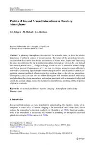
Figure 1: Rayleigh (top, linear scale, d = 20nm, λ = 450nm) and Mie (bottom, logarithmic scale, d = 4µm, λ = 450nm) phase functions for θ ∈ h0, πi. The corresponding polar plots are shown as well.

major advantage is that it is directly useful for procedural evaluation in programming languages such as C++. 3.2.1

Phase function

Phase function denotes an angular dependency of scattered light in respect to the original direction of incoming light. It is a 1D function that takes as its parameter the scattering angle θ (the angle between the incoming light ray and the scattered light ray) and returns the relative amount of scattered light under that particular angle. For Rayleigh scattering, the phase function is defined as 3 FR = (1 + cos2 (θ )). 4

(2)

The function is symmetrical around the axis of incindent light and follows from wave properties of electromagnetic radiation (see Figure 1). On the other hand the Mie phase function FM (θ ) is very complex and can not be calculated by a single analytic equation. It generally contains a strong forward lobe and many side and backward lobes and changes with the diameter of the scattering particle. However, after the size of the scattering particle exceeds the wavelength of scattered light, a strong prevalence of the dominating forward lobe arises. Thanks to this, it can be approximated by Henyey-Greenstein function further improved by Cornette and Shanks [2]: FM (θ , g) =

3(1 − g2 ) (1 + cos2 (θ )) 2 2(2 + g ) (1 + g2 − 2g cos(θ ))3/2

(3)

where g ∈ (−1; 1) is an assymetry factor denoting the width of the forward lobe (see Figure 3). 3.2.2

L Pc

Scattering coefficient

(1)

Is

Let’s define a Rayleigh/Mie particle polarisability constant αR,M as 2π 2 (n2e − 1)2 (4) αR,M = 3Ne2R,M where ne is the index of refraction of the Earth’s atmosphere at sea level and NeR,M is the Rayleigh/Mie particles’ molecular number density of the Earth’s atmosphere at sea level. This constant is calculated from measured parameters of the Earth’s atmosphere and denotes how well the particle scatters the light. The Rayleigh and Mie scattering coefficients βR (λ ) and βM () are then defined as NR αR λ4 βM () = 4πNM αM

βR (λ ) = 4π

The Rayleigh/Mie scattering intensity IsR,M expresses the amount of light deviated by a given angle θ during a scattering event at point P (see Figure 2 for illustration). It depends on spectral wavelength λ and is expressed by the following equation: (7)

where II (λ ) is the spectral intensity of incident light and ρR,M (h) is the Rayleigh/Mie density function. This function expresses the decrease of atmospheric density in dependence on h, the altitude of P over the ground. It is defined as follows: h ρR,M (h) = exp(− ) (8) HR,M where HR ≈ 8000m and HM ≈ 1200m are the Rayleigh and Mie scale heights. These express the altitude where the density of an appropriate type of particles scales down by a 1/e term. 3.2.4

Transmittance

Transmittance, or optical length, tR,M (S, λ ) expresses the amount of attenuated light with wavelength λ after it passes the distance S in a Rayleigh/Mie scattering medium. It is defined by the equation Z S

tR,M (S, λ ) = βR,M (λ )

0

ρR,M (s0 )ds0 .

(9)

Attenuation is the consequence of out-scattering in participating medium.

Pb

V

P

θ

atmosphere

h

s

PO ~ Pa

planet

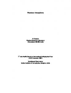
Figure 2: A schematic view of the atmosphere 3.2.5

Single-scattering

The single-scattering equation describes the intensity of (1) light ISR,M (PO ,V, L, λ ) that reaches an observer PO looking in the direction V , after exactly one scattering event: ISR,M (PO ,V, L, λ ) = II (λ )FR,M (θ ) ·

(6)

Scattering intensity

IsR,M (λ , θ , P) = II (λ )ρR,M (h)FR,M (θ )βR,M (λ )

δ

(k)

Is

(1)

(5)

where NR,M denotes molecular number density of Rayleigh/Mie particles in the desired atmosphere. Note that βM () is λ -independent. 3.2.3

N

s'

Z Pb Pa

βR,M (λ ) · 4π

(10)

ρR,M (h) exp(−tR,M (PPc , λ ) − tR,M (Pa P, λ ))ds

where L is the direction to the light source and h is the altitude of sample point P, which is parameterized by s. Pa and Pb are the first and the last point where the density of the atmosphere is nonzero (when the observer is situated inside the atmosphere, then Pa = PO ). Pc is the intersecting point of L with the upper atmospheric boundary when starting in P (see Figure 2 for illustration). FR,M (θ ) can be excluded from the integration, because we assume that all light rays coming from the light source are parallel. (1) Finally, the total intensity of single-scattered light IS is obtained by the sum (omitting parameters for shortness): (1)

(1)

(1)

IS = ISR + ISM .

3.2.6

(11)

Multiple scattering

The key to make calculation of multiple scattering possible (on consumer hardware) is to avoid the most primitive way of doing it. This way corresponds to a multidimensional integral which is in fact a global illumination equation in a participating medium. The higher scattering orders would be obtained here by nested recursive integration, the evaluation of which would take a very long time. The solution to this is the formulation of the reccurent formula that would somehow take advantage of the previously calculated data. At first we define a gathered scattered light of k-th order (k) GR,M (P,V, L, λ ) at some point in the atmosphere P in the direction V when the light source is in the direction L as (k)

GR,M (P,V, L, λ ) =

Z 4π

(k)

FR,M (θ )ISR,M (P, ω, L, λ )dω (12)

where θ is the scattering angle between V and ω and (k) ISR,M (P, ω, L, λ ) is the scattered light intensity of kth order. This formula denotes the amount of gathered light,

which has undergone exactly k scattering events, reflected (in-scattered) into the direction −V at P. We can now define the scattered light intensity of kth (k) order ISR,M (PO ,V, L, λ ) at the observer position PO in the direction V as (k)

ISR,M (PO ,V, L, λ ) = ·

Z Pb Pa

βR,M (λ ) · 4π

(13) (a)

(k−1) GR,M (P,V, L, λ )ρR,M (h) exp(−tR,M (Pa P, λ ))ds

where the notation stays similar to Equation 10. Again the total intensity of the kth order of scattered light is ex(k) (k) (k) pressed as IS = ISR + ISM . If we now define K as the number of desired calculated scattering orders, we get the total scattering intensity as K

(k)

IS = ∑ IS .

(14)

i=1

4

Method description

4.1

Precomputation

The rendering part of our algorithm is intended to be run on graphics hardware. Since this is not capable of working with textures of more than three dimensions, it is important to keep the dimensionality of our lookup table in this limit. Also it is necessary to keep the sampling resolutions in all dimensions within reasonable limits, so the size of the lookup table does not grow too large. 4.1.1

Parameterization

The precomputation of Equation 14 for every observer position PO [x, y, z], every view direction V [x, y, z] and every light source direction L[x, y, z] would require a 9dimensional table, which is by far unaffordable. It’s necessary to take advantage of some symmerties as well as make a few assumptions: • (1) The star (light source) is so far away that all light rays from it can be considered parallel

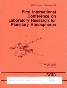
Figure 3: The plot of Cornette’s FM for g = −0.95 (a) and the correct sampling of Mie scattering after deferring evaluation of FM (b)

Thanks to the assumptions (2) and (4), we can reduce PO , V and L into 4 scalar parameters — altitude h ∈ h0; Htop i (where Htop is the upper atmosphere boundary altitude), view↔zenith angle φ ∈ h0; πi, sun↔zenith angle δ ∈ h0; πi and sun↔view azimuth ω ∈ h0; πi. Although it is possible to emulate 4D table with 3D table, we decided to omit azimuth ω from precomputation, because of the following reasons: • The main product of incorporation of ω into precomputation is the presence of the planet’s shadow during the sunset in those parts of the sky where there is no direct illumination. This shadow is however only weakly visible (due to multiple scattering) and in most times it is masked by the horizon. • The size of the precomputed table is decreased several times thanks to this. However, this omitting also causes uniformity of the atmospheric colour in respect to ω, because all view directions now have implicitly ω = 0. The solution to this is described in Section 4.1.2. Our task is now to remap parameters of our lookup table h, φ and δ into the 3D texture coordinate space UVW , i.e. to design a remapping function f : h0; Htop i × h0; πi × h0; πi −→ h0; 1i × h0; 1i × h0; 1i. For this purpose we partially adopted the remapping functions from [1]: q (h2 − R2p )/(R2a − R2p ) U =

• (2) The planet is perfectly spherical (neglecting terrain morphology for now) • (3) The density of the atmosphere is changing in respect to altitude (according to ρR,M (h)) but not in respect to latitude and longitude (currently the strongest limitation — it binds us to one type of atmosphere, until the precomputation step is repeated) • (4) The atmosphere is a spherical shell and its colour is symmetrical around the plane between L and the zenith vector in PO

(b)

V

= (1 + cos(φ ))/2

W

= (1 − e−2.8 cos(δ )−0.8 )/(1 − e−3.6 )

where R p and Ra are the planet and the atmosphere radius, respectively. 4.1.2

Phase function

Thanks to the assumption (1) we can not only exclude evaluation of FR,M from integration in Equation 10, but we can even defer its evaluation into a fragment shader. This has two advantages.

Firstly, it partially solves the problem with the absence of ω in our parameterization, because now it is accounted for at least in calculation of FR,M (because ω is contained within the angle between V and L). Even though ω is not contained in the rest of the computations, the uniformity of atmosphere colour in respect to it now does not appear so strongly. Secondly, it solves the problem of undersampled Mie scattering. The gradient of Mie-scattered light is very high when the angle between V and L is close to zero because of the behaviour of Cornette’s approximation of FM (see Figure 3 for its visualization). Deferring calculation of FM gives us a very fine per-fragment sampling precision. Deferred phase function for Rayleigh scattering causes unnatural look of the atmosphere, because the standard Rayleigh phase function has its maxima at 0◦ and 180◦ angles and its minimum at 90◦ angle (see Figure 1). Normally, this behaviour is neutralised by multiple scattering, but here the phase function is applied also on higher scattering orders. For this purpose we derived an ad hoc Rayleigh phase function   8 7 1 + cos(θ ) (15) FR (θ ) = 10 5 2

Figure 4: Comparison of single-scattering (left column) and multiple scattering (right-column) from identical views.

that looks more natural, as it has its minimum at 180 degrees. The darkest area of the sky during the sunset is then on the opposite side of the sky than the sun.

4.2

4.1.3

Multiple scattering

Calculation of higher scattering orders by direct evaluation of Equation 13 would cause the same exponential computational complexity (in regard to the number of scattering orders K) as the forward recursive computation. The key to success is the fact that Equation 13 is formulated in the way that it allows an incremental computa(1) tion of scattering orders, one at the time. At first the IS is computed exactly, according to Equation 11 and the results of this computation are stored in the lookup table as described in Section 4.1.1. Then we can compute the desired number of higher scattering orders — for calculation of (k) the IS we use Equation 13, where G(k−1) is calculated by fetching scattering intensity values from the already computed lookup table for (k − 1)th scattering order. When we have all desired scattering orders computed, we just sum them according to Equation 14 into a single lookup table. 4.1.4

Ambient illumination

Scattered light indeed causes ambient illumination on the planetary surface and it is necessary to account for this in order to conserve energy in the simulated system. The intensity of the ambient illumination on the planetary surface due to scattered light IA (L, λ ) for the light source direction L can be expressed by Z

IAR,M (L, λ ) =

2π

(N • ω)ISR,M (0, ω, L, λ )dω

(16)

where N is the surface normal. This can be precomputed into a 1D lookup table by fetching intensity values from the main scattering 3D lookup table.

Rendering

As has been said, the rendering part is intended to be processed by graphics hardware. All lookup tables are represented by textures that are utilisable by GPU. The atmosphere is represented by a single tesselated sphere and is always rendered with front face primitive culling enabled. All important computations are carried out in a fragment shader, which also fetches values from the precomputed lookup textures. Fetching from the main lookup texture is performed by calculating an inverse function from the remapping projection f .

4.2.1

Planetary surface

For rendering the planetary surface we have to account for direct illumination, indirect illumination and in case of water surfaces, for reflected skylight. For calculation of the direct illumination, the incident light at the top of the atmosphere must be attenuated by the optical length on its path through the atmosphere, because of out-scattering: II0 (Ps , L, λ ) = II (λ ) exp(−(tR + tM )(Ps Pc , λ ))

(17)

where II0 (Ps , L, λ ) is the direct illumination intensity at surface point Ps , L is the light direction and Pc is the intersection of L with the upper atmosphere boundary (see Figure 5). To avoid costly real-time calculation of transmittance, it is also possible to precompute it into a 2D lookup table

N R

piece of the puzzle, we can now express the total amount of light reflected from the planetary surface that reaches the observer as

L Pc

Pa PO

IP (PO ,V, L, λ ) =

IW IP

φ φ

IA

Ps

I'I

+IC (λ )(IAR + IAM )(L, λ ) + (20) ˆ +aF(ϕ)(I WR + IWM )(Ps ,V, L, λ ) ) ·

atmosphere

· exp(−(tR + tM )(PO Ps , λ ))

planet

Figure 5: A scheme illustrating the calculation of the light reflected from the planetary surface parameterized by the observer altitude h and zenith angle µ. Each record (texel) in this table then stores tR,M (PPc ), where the point P has an altitude h and Pc is the intersection of the ray that starts at P under a zenith angle µ, with the upper atmosphere boundary. Obtaining the indirect illumination is trivial here, having precomputed the abmient intensity lookup texture. Only one texture fetch is necessary here for obtaining IAR,M (L, λ ). If Ps is located on a water surface, we must also account for the reflection of the sky. Thanks to the nature of the scattering lookup table, we can easily fetch the sky reflection IWR,M (Ps ,V, L, λ ) from here, without resorting to any costly multi-pass technique. At first we calculate the reflection vector R at Ps . Then we set h = 0, ϕ to the zenith angle of R and δ to the zenith angle of L at Ps . Then we fetch the main scattering lookup table by evaluating the inverse remapping function. For obtaining the reflected amount of light, one should use the Fresnel reflectance term for unpolarised light. However, this is not necessary for non-absorbing or weakly absorbing substances like water, as the imaginary part of their index of refraction is zero or very small, respectively3 . For this reason and also for the sake of decreasing the computational requirements, we use the following approximation: ˆ F(ϕ) = max(0.03, (1 − cos(ϕ))5 )

(18)

where ϕ is again the zenith angle of R. This simple and cheap formula fits very well with the actual Fresnel reflectance of water. Finally, to calculate the total intensity of light reaching the observer situated at PO , we have to calculate the transmittance from Ps to PO . Such value is however not stored in our lookup table for transmitance, because it stores the transmittance value from some altitude always to the top of the atmosphere. To obtain tR,M (PO Ps , λ ) we must perform two transmittance texture lookups: tR,M (PO Ps , λ ) = tR,M (Pa Ps , λ ) − tR,M (Pa PO , λ )

( IC (λ )(N • L)II0 (Ps , L, λ ) +

(19)

where Pa is the intersection of the inverted view ray −V with the upper atmosphere boundary. Having this last 3 The imaginary part of the index of refraction of water is in the orders from 10−10 to 10−8 in the visible spectrum

where IC is the diffuse colour of the planet’s surface at Ps and a is the surface albedo at Ps . For water surfaces, IC is generally blue and can be regarded as a rough substitution for the calculated intensity of underwater scattering. We do not discuss here the rendering of a complex terraing morphology, since this has not been amongst the topics of our work. If you are interested in how to utilise the main scattering lookup table precomputed for a perfectly spherical planet in a terrain renderer, please refer to [1], or [10]. 4.2.2

Star disc rendering

In order to keep the scene looking natural, it is necessary to also render a star (light source) disc. It is however sufficent to use a simple textured billboard for this purpose — this billboard then always has to be rendered in the light source direction. Shading of the disc is then identical with the calculation of the direct surface illumination (Equation 17), only the II (λ ) term is changed with the colour fetched from the billboard texture (although these should be similar) and the observer current position PO is substituted for the surface point Ps .

5

Results and Conclusions

Our implementation uses a single-thread CPU-based program for the precomputation algorithm and a GPU-based renderer. The precomputation could be also carried out by a GPU, but we have chosen CPU-implementation because of its flexibility and higher numerical precision. The used resolutions of the lookup textures are 32 × 256 × 32 × 64bpp for the main scattering 3D texture, 512 × 512 × 64bpp for the transmittance 2D texture, 4096 × 32 × 32bpp for the phase function 2D texture and 256 × 64bpp for the ambient 1D texture. Their size together is 5MB. For numerical sampling of all integrals a trapezoidal evaluation rule with 30 evenly distributed samples for each integral was used. Using higher sampling rates does not improve the apparent quality of the calculated data. The hardware configuration used for testing was a desktop PC with Intel Core 2 Duo 1.86 Ghz CPU, NVidia GeForce 8800GT graphics adapter and 2GB DDR2 RAM. The precomputation time for the entire dataset was about 3 hours for 6 scattering orders when using the aforementioned sampling rates. The performance of our rendering application is always in real-time framerates. For

the screen resolution of 1024 × 768 the average measured framerate was 180 FPS and the minimal framerate was 85 FPS. For the screen resolution of 2560 × 2048 the average measured framerate was 62 FPS and never dropped below 33 FPS. The scene in both measurement cases contained approximately 530,000 vertices. For the results of our method, see Figure 4, Figure 6 and the title page.

References [1] Bruneton E., Neyret F.: Precomputed Atmospheric Scattering, in Comput. Graph. Forum: Proceedings of the 19th Eurographics Symposium on Rendering 2008, volume 27, number 4, pages 1079–1086, 2008 [2] Cornette W. M., Shanks J. G.: Physical Reasonable Analytic Expression for The Single-Scattering Phase Function, in Applied Optics Vol. 31, No. 16, pages 3152–3160, 1992 [3] Haber J., Magnor M., Seidel H.-P.: Physically-Based Simulation of Twilight Phenomena, in ACM Transactions on Graphics, Vol. 24, No. 4, pages 1353–1373, 2005 [4] H. C. van de Hulst: Light Scattering by Small Particles, Dover Publications, New York, ISBN 0-48664228-3, 1981 [5] Nishita T., Dobashi Y., Kaneda K., Yamashita H.: Display Method of the Sky Color Taking into Account Multiple Scattering, in Pacific Graphics ’96, pages 66–79, 1996 [6] Nishita T., Sirai T., Tadamura K., Nakamae E.: Display of The Earth Taking into Account Atmospheric Scattering, in Siggraph ’93: Proceedings of the 20th annual conference on Computer graphics and interactive techniques, pages 175–182, 1993 [7] O’Neil S.: Real-Time Atmospehric Scattering, http://www.gamedev.net/reference/ articles/article2093.asp, 2004

Figure 6: Examples of different atmospheres’ parameterizations. Left column: 5-times sparser atmosphere than the Earth’s, right column: 5-times denser atmosphere than the Earth’s. Top to bottom: global view, fisheye view from altitude 20km, sunset from altitude 1km.

Conclusion We have presented a method for real-time rendering of parameterizable planetary atmospheres. At first we have shown a physically-based mathematical model for calculation of atmospheric light scattering, accounting for both single and multiple scattering. Secondly, we have described the procedure for precomputing this model into a set of lookup tables. Then we have shown how to utilise these lookup textures in a real-time renderer for rendering of the planet and its atmospheric shell. Finally we have verified our method with a functional implementation.

6

Acknowledgements

I would like to thank Petr Kmoch for his kind guidance during the creation of this work.

[8] O’Neil S.: Accurate Atmospheric Scattering, Addison-Wesley Professional, in GPU Gems 2: Programming Techniques for High-Performance Graphics and General-Purpose Computation, pages 253– 268, 2005 [9] Preetham A. J., Shirley P., Smits B.: A Practical Analytic Model for Daylight, in Siggraph ’99: Proceedings of the 26th annual conference on Computer graphics and interactive techniques, pages 91–100, 1999 [10] Schafhitzel T., Falk M., Ertl T.: Real-Time Rendering of Planets with Atmospheres, in Journal of WSCG, volume 15, 2007 [11] Wenzel C.: Real-time atmospheric effects in games, in ACM Siggraph 2006’s International Conference on Computer Graphics and Interactive Techniques: Advanced real-time rendering in 3D graphics and games, pages 113–128, 2006 [12] Zotti G., Wilkie A., Purgathofer W.,: A Critical Review of the Preetham Skylight Model, in WSCG 2007 Short Communications Proceedings I, pages 23–30, 2007