Renormalization Group and Ward Identities in regularized QED4 with

Renormalization Group and Ward Identities in regularized QED4 with large photon mass Vieri Mastropietro Universit` a di Roma “Tor Vergata” via della Ricerca Scientifica, I-00133, Roma

Abstract. We analyze, by Renormalization Group methods, a regularized version of Euclidean QED4 with any value, including zero, of the fermion mass and a large photon mass. We will prove that the Schwinger functions are expressed by convergent series and verify the Ward Identities up to corrections which are small for momentum scales far from the ultraviolet cut-off. Keywords QED; Ward Identities; Renormalization Group; Constructive QFT. PACS numbers 12.20.-m; 11.10.Gh

1. Introduction 1.1 Ward Identities and Renormalization Group The gauge invariance of classical Electrodynamics leads to well known difficulties in its quantization, and the standard method to overcome them consists to add to the action a gauge-fixing term ξ(∂ µ Aµ )2 ; particularly convenient is the choice ξ = 1/2 so that the photon propagator aquires the simple form δ µ,ν v(p) with v(p) = (p2 + M 2 )−1 , where M is a photon mass which can be added to make the infrared problems less severe. The formal Euclidean generating function of QED4 then becomes A

¯

eW (Jµ ,φ,φ) =

Z

− ¯ dψdψdAe

R

¯x (−γµ ∂µ +γµ Aµ,x )ψx +J A Aµ,x +φx ψ ¯x +φ ¯x ψx ] dx[ 14 Fµ,ν,x Fµ,ν,x + 21 (∂µ Aµ,x )2 + 21 M 2 Aµ,x Aµ,x +ψ µ,x

(1.1) and the gauge invariance of the classical theory is replaced by a weaker invariance charapterized by the validity of an infinite set of non trivial identities between the correlations, called Ward Identities (WI) [W],[T], like −ipµ hAµ,p ψk ψ¯k−p i = ev(p)[hψk−p ψ¯k−p i − hψk ψ¯k i]

(1.2)

and similar ones with any number of fields, obtained from (1.1) with the change of variables ψ → e iχx ψx , ψ¯x → ψ¯x e−iχx . The WI can be also obtained by Feynman graph expansions, using that the fermionic propagator verify 1 1 1 1 − = 6p (1.3) 6 k 6 k+ 6 p 6 k (6 k+ 6 p) or using an operatorial approach, from the relation ∂µ hjzµ ψx ψ¯y i = h∂µ jzµ ψx ψ¯y i + δ(z0 − x0 )h[jz0 , ψx ]ψ¯y i − δ(z0 − y0 )hψx [jz0 , ψ¯x ]i = δ(z − x)hψx ψ¯y i − δ(z − y)hψx ψ¯y i (1.4) where the delta functions arise from the derivative of the θ-functions of the time order product and in the last step one uses the conservation of the current ∂µ jzµ = 0 and the commutation relation δ(z0 − x0 )[jz0 , ψx ] = δ(z − x)ψx . Of course all such derivations of the WI are purely formal, and indeed the correlations appearing in the r.h.s. or the l.h.s. of (1.2) are plagued by ultraviolet divergences. In order to construct a quantum gauge theory like 19/maggio/2007; 14:57

1

QED one has to regularize the theory introducing cut-offs, and then prove that, with a proper choice of the bare parameters, the cut-offs can be be removed and the correlations not only verify the Osterwalder-Schroeder axioms, but also the infinite set of WI associate to the gauge symmetry. By using regularizations respecting (1.3), like the dimensional one, a classical inductive computation shows that the Ward Identities, understood as identities valid order by order in the perturbative expansion, are preserved through the renormalization procedure, see for instance [IZ]. More complex is to prove a similar statement with the momentum regularizations used in the Wilsonian Renormalization Group approach to QFT, introduced in [P] and [G], which has on its side the merit to be suitable in principle for the non-perturbative construction of QFT models. For finite values of the cut-offs, the momentum regularizations violate (1.3) and produce additional terms in the WI, so that one has to show that WI are finally restored removing the cut-offs. This was proved in [FHRW], as an order by order statement, by using the Gallavotti-Nicolo’ tree formalism with two different regularizations, namely a momentum and a Pauli-Villar loop regularization; later on in [H] a similar statement was proved by using only momentum regularizations, assuming a non-vanishing photon mass. The renormalizability of QED4 and the restoration of the WI removing the cut-offs was also obtained in [KK1] and [KK], respectively with massive or massive photons, using the Polchinski method. The interplay between WI and Wilsonian Renormalization Group in gauge theory has been also extensively analyzed in the physical literature, see for instance [B], [BAM]. In all the above analysis, QED is studied at a perturbative level, writing the n-point functions as formal power series whose convergence cannot be proved and which are probably not convergent at all; the WI are proved as order by order identities among formal series expansions. It is generally believed that a non-perturbative construction of QED4 , with no cut-offs, is possible only considering it as part of the Electroweak theory, which is asymptotically free. A non-perturbative construction of QED4 with an ultraviolet cut-off was achieved in [DH]: the fermionic fields can be integrated out obtaining an effective boson theory which can be studied by cluster expansion techniques. Under the assumption of massless photons and that the fermionic mass is much larger than the electric charge, it was shown that the theory is asymptotically free in the infrared, that is that the behaviour of the photon n-point functions is the same as in the free case. The properties of the WI were however not analyzed; indeed they appear quite involved to study once that the fermionic degree of freedom are integrated out. In this paper a regularized version of QED4 is analyzed at a non-perturbative level following the opposite route, that is by integrating out the photon fields; in this way a purely fermionic theory is obtained which can be considered a non-local version of the Jona-Lasinio model. We assume a large photon mass, but our results are valid also for a small or even vanishing fermionic mass; note that the electron mass-charge ratio in adimensional units is O(10−20 ) so that the requirement of large mass with respect to charge is quite unrealistic. The use of a fermionic formalism makes possible the study of the WI. We will show that the WI are verified up to corrections which are small for momentum scales far from the ultraviolet cut-off, provided that the charge renormalization is taken into account. Such results will be proved by an extension of the methods previously adopted in d = 2 QFT [M],[BFM] (and based on [BM],[BM1]), where they allow the removal of the ultraviolet cut-off and the complete construction of a non-trivial theory. 1.2 Main results. We consider the following generating function Z R A ¯ eWN,L (J ,φ) = P (dψ)P (dA)e

¯x (Aµ,x γµ )ψx +J A Aµ,x +φx ψ ¯x +φ ¯x ψx ] dx[eψ µ,x

(1.5)

where -)in Λ = [0, L] × [0, L] × [0, L] × [0, L] a lattice Λa is introduced whose sites are given by the space-time points xµ = nµ a, µ = 0, 1, 2, 3 with L/a integer and nµ = −L/2a, 1, . . . , L/2a − 1. We also consider the set D of space-time momenta k with kµ = (mµ + 21 ) 2π L and with mµ = 0, 1, . . . , L/a − 1. -)The γ-matrices verify {γµ , γν } = −2δµ,ν and are chosen as       0 iI 0 −σα I 0 0 α 5 γ = , γ = , γ = . (1.6) iI 0 σα 0 0 −I

19/maggio/2007; 14:57

2

and σ α , α = 1, 2, 3, are the σ-matrices   0 1 1 σ = , 1 0

2

σ =



0 −i i 0



,

3

σ =



1 0 0 −1



.

(1.7)

-)With each k ∈ D we associate two Grassmann spinors ψk , ψ¯k , and we define the functional integration Dψ as the linear functional on the Grassmann algebra generated be the variables ψk , ψ¯k such that, given a monomial Q Q(ψ) in the variables ψk , ψ¯k ,Rits value its zero except in the case Q(ψ) = k∈D ψk ψ¯k , up to a permutation of P P Q 1 −ikx ¯ ψk and ψ¯x = L14 k∈D eikx ψ¯k the variables; in such a case k∈D e k∈D ψk ψk = 1. We define ψx = L4 and the fermionic integration is ZN X ¯ −1 ψk χN (k)(i 6 k + mI)ψk ] (1.8) P (dψ (≤N ) ) = N −1 Dψ exp[− 4 L k∈D

where 6 k = γµ kµ and χN (k) is a non-vanishing smooth cut-off function, never vanishing and selecting momenta |k| ≤ γ N ; a specific choice will be done in the following section. The propagator corresponding to (1.8) is 1 X −i 6 k + mI −ik(x−y) g(x − y) = 4 e χN (k) (1.9) L k2 + m 2 k∈D

¯ µ ψ and j 5 = ψγ ¯ µ γ5 ψ. We will call jµ = ψγ µ -)For any x ∈ Λa , Aµ,x is an euclidean boson field defined by the Gaussian measure P (dA) with covariance vµ,ν (x − y) = δµ,ν v(x − y). We will consider the case v(x − y) =

1 X −ip(x−y) χN (p) e 2 L4 p2 + M N

(1.10)

p∈D

with MN = γ N M . The Schwinger functions are defined by hψx1 ; ...; ψxn ; ψ¯y1 ; ..; ψ¯yn ; Aµ1 ,z1 ; ...; Aµm ,zm i = We will prove the following result.

¯ N,L(J A , φ) ∂ 2n+m W A A ¯ ∂φx1 ...∂φxn ∂ φy1 ...∂φyn ∂Jµ1 ,z1 ...∂Jµm ,zm J=φ=0

(1.11)

Theorem.There exists ε0 , independent from m, N , such that the Schwinger functions (1.11) are analytic in |e| ≤ ε0 and verify the Ward Identity, for |p|, |k|, |k − p| ≤ κ −ipµ hAµ,p ; ψk ψ¯k−p i = e0 v(p)[hψk−p ψ¯k−p i − hψk ψ¯k i](1 + O(eκγ −N ))

(1.12)

where e0 = e(1 − c+ e2 + O(e4 )) where c+ is a constant given by (4.4),(4.6) below. In the massless case m = 0 the following chiral Ward Identity holds 5 (1.13) −ipµ hjµ,p ; ψk ψ¯k−p i = a(hψk−p ψ¯k−p i − hψk ψ¯k i)[1 + O(e(κγ −N )θ )] with a = 1 + O(e2 ) and θ > 0 is a constant. Remarks 1)(1.12) says that the WI (1.2) is verified up to corrections O(e(κγ −N )θ ) , provided that the bare charge e is replaced by the dressed charge e0 ; a similar statement holds for all the other WI and it could be proved by a straightforward extension of the analysis in this paper. 2)As a consequence of (2.4), (1.12) can be written as a conservation equation −ipµ hjµ,p ; ψk ψ¯k−p i = a ¯(hψk−p ψ¯k−p i − hψk ψ¯k i)[1 + O(e(κγ −N )θ )] 19/maggio/2007; 14:57

3

(1.14)

¯ µ ψ and the axial current as e0 ψγ ¯ µ γ 5 ψ, we see that with a ¯ = 1 − c+ e2 + O(e4 ); if we define the current as e0 ψγ (1.14) and (1.12) are compatible with the current conservation (up to small corrections) but not with the axial current conservation; this is the well known anomaly in QED4 . 3)Our results hold also for the Jona-Lasinio model, whose Schwinger functions are given by (1.11) with v(x − y) = λδ(x − y), assuming λ = O(γ −2N ). 4)The value of the bare photon mass MN should be chosen to make vanishing the photon mass at physical scales; a second order perturbative computations says that the renormalization of the photon mass is O(γ N e). While it has the N -dependence we assumed in (1.10), the choice M = O(e) is outside the range of validity of our theorem. 5)In the N → ∞ a non-interacting (trivial) theory is found, with fermionic wave function renormalization (1) ZN = 1 + O(e) and current renormalization ZN = 1 + O(e).

2. Renormalization Group analysis 2.1 Multiscale Integration We will consider for notational simplicity the m = 0 case; the massive case poses no additional difficulty and it can be analyzed in a similar way up to some trivial modifications (see for instance [BFM] for the d = 2 case). Integrating the bosonic variables A one can rewrite (1.5) as a purely fermionic theory e

¯ N,L (J A ,φ) W

=

Z

1

P (dψ)e 2

R

¯x γµ ψx +J A ][eψ ¯y γµ ψy +J A ]+ dxdyv(x−y)[eψ µ,x µ,y

R

¯x +φ ¯x ψx ] dx[φx ψ

(2.1)

R P where dx is a shorthand for a4 x∈Λa . We will find more convenient to consider the following generating function, writing λ = e 2 /2 eWN,L(J,φ) =

Z

P (dψ (≤N ) )e−V

where V (N ) = −λ

Z

(N )

(ψ)+

R

¯x γµ ψx + dxJµ,x ψ

R

¯x +φ ¯x ψx ] dx[φx ψ

dxdyv(x − y)(ψ¯x γµ ψx )(ψ¯y γµ ψy )

(2.2)

(2.3)

Of course the correlations obtained from (2.2) are trivially related to the correlations from (2.1) (see for instance (2.4)); for instance ev(p)hjµ,p ; ψk ψ¯k+p i = hAµ,p ; ψk ψ¯k+p i (2.4) WN,L is invariant under the Euclidean transformation ψ 0 (x0 ) = S(Λ)ψ(x)

−1 ¯ ψ¯0 (x0 ) = ψ(x)S(Λ)

x0ν = Λµ,ν xν

with S(Λ)γ ν S(Λ)−1 = (Λ−1 )µ,ν γν . The local quadratic invariant terms are then only ψ¯x ψx and ψ¯x 6 ∂ψx . We describe in more detail our choice of the cut-off fuction χN (k). Let χ0 ∈ C ∞ (R+ ) be a non-negative, non-increasing smooth function such that χ0 (t) =



1 if 0 ≤ t ≤ 1 0 if t ≥ γ0 ,

for any choice of γ0 : 1 < γ0 ≤ γ; and we define, for any integer k

19/maggio/2007; 14:57



fk (k) = χ0 γ −k |k| − χ0 γ −k+1 |k| 4

(2.5)

−1 and fk (k) are functions with support γ k−1 ≤ |k| ≤ γ k+1 , so that CN (k) = N +1 cut-off function vanishing for |k| ≥ γ . We define N X

ε χN (k) = CN (k)−1 =

PN

k=−∞

fk (k) is a compact support

fkε (k)

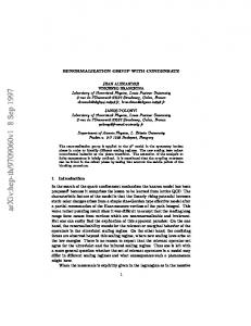
k=−∞ ε ε where fkε (k) = fk (k) for −∞ ≤ k ≤ N − 1, while fN (k) is a C ∞ function of |k|, such that fN (k) = fN (k) for γ N −1 ≤ |k| ≤ γ N , fN (k) > 0 for |k| ≥ γ N and, if |k| ≥ γ N +1 , 0 < |k| ≤ e−|k| .

Fig. 1

γN

|k|

γ N +1

Fig 1: Graphical representation of χN (k) The functional integral is analyzed through a multiscale integration procedure; the starting point is to write the fermionic propagator as N X g(x − y) = g (h) (x − y) (2.6) h=−∞

with, by integrating by parts, for any positive integer K |g (h) (x − y)| ≤ γ 3h

CK 1 + (γ h |x − y|)K

(2.7)

In a similar way the following bound for the boson propagator is obtained: |v(x − y)| ≤ γ 2N

CK 1 + (γ N |x − y|)K

(2.8)

By well known properties of Grassmann integrals (see for instance [GM]) we can write Z Z R R (≤N ) (≤N ) (≤N ) (≤N ) (N ) (≤N ) ¯x ¯x ¯x ψx )+ dxJµ,x ψ γ µ ψx + dx[φx ψ +φ ] WN,L (J,φ) (≤N −1) e = P (dψ ) P (dψ (N ) )e−V (ψ

(2.9)

−1 ε where P (dψ (N ) ) and P (dψ (≤N −1) ) are Grassmann integrations given by (1.9) with CN (k) replaced by fN (k) PN −1 −1 (N ) and CN −1 (k) = k=−∞ fj (k) respectively (and ZN replaced by 1). We can integrate the field ψ obtaining

e

WN,L (J,φ)

=e

−L4 EN +SN (φ,J)

Z

P (dψ (≤N −1) )e−V

(N −1)

(ψ (≤N −1) )+B(N −1) (ψ,J,φ)

(2.10)

¯ as where V (N −1) is the effective potential which can be written , if ψ ε is ψ or ψ, V (N −1) (ψ (≤N −1) ) =

XZ

(N −1)

dx1 ...dx2l W2l

(x1 , .., x2l )

2l Y

ψx(εii ≤N −1)

(2.11)

i=1

l,m

and B (N −1) is the effective source, which can be written as (N −1)

B (N −1) (ψ, J, φ) = B1 19/maggio/2007; 14:57

(N −1)

(ψ (≤N −1) , J) + B2

5

(N −1)

(ψ (≤N −1) , φ) + B3

(ψ (≤N −1) , J, φ)

(2.12)

(N −1) (N −1) (N −1) where B1 contains all the terms linear in J, B2 all the terms linear in φ or φ¯ and B3 is the rest. We split the effective potential V (N −1) as LV (N −1) + RV (N −1) , where R = 1 − L and L is a linear operator (N −1) (N −1) acting on functions like (2.11). Its action on the kernels W2l is LW2l = 0 if l > 1,while if l = 1

L

Z

(N −1)

dxdyW2

Note that by parity a scalar so that

R

(N )

dyW2

(x, y)ψ¯x ψy =

Z

(N −1)

dxdyW2

(x, y)[ψ¯x ψx + (xµ − yµ )ψ¯x ∂µ ψx ]

(2.13)

R (N ) (x, y) = 0 and by Euclidean invariance dy(xµ − yµ )W2 (x, y) = γµ S with S Z (2.14) LV (N −1) = zN −1 dxψx 6 ∂ ψ¯x

(N −1)

Analogously B1 (ψ (≤N −1) , J) is given by an expression similar to (2.11), sum of momonials with l Grassmann (N −1) (N −1) fields and a single γµ Jµ fields, integrated over kernels W2l,1 . We define the L operation as LW2l,1 = 0 if l > 1 and if l = 1 Z Z (N −1) (N −1) (z, x, y)γµ Jµ,z ψ¯z ψz (2.15) L dxdydzW2,1 (z, x, y)γµ Jµ,z ψ¯x ψy = dxdydzW2,1 and again by Euclidean invariance (N −1) LB1 (ψ, J)

It is convenient to write R Z

(N −1)

dxdydzW2,1

Z

=

(1) ZN −1

(N −1)

dxdydzW2,1

(z, x, y)γµ Jµ,z [(xµ − zµ )

Z

Z

dzJµ,z ψ¯z γµ ψz

(2.16)

(z, x, y)γµ Jµ,z ψ¯x ψy =

1

dt∂µ ψ¯x(t) ψz + (yµ − zµ )

0

Z

1

dtψ¯x ∂µ ψy(t) ]

(2.17)

0

where x(t) = x + t(z − x) and y(t) = y + t(z − y) are called interpolated points; a similar expression holds for (2.13). (N −1) B2 (ψ (≤N −1) , φ) has the form   i Z ∂ (N −1) ∂ (N −1) (N ) (≤N −1) (≤N −1) (N ) ¯ ¯ ¯ = dx φx ψx + ψx φx + dxdy φx g (x − y) V + ¯ V g (x − y)φx ∂ψy ∂ ψy (2.18) (N −1) (N −1) (N −1) and the L operation is defined decomposing in (2.18) V as LV + RV using the definition in (N −1) (2.13). Finally we define LB3 = 0. We write then Z (N −1) 4 WN,L (J,φ) −L4 EN +SN (φ,J) e =e P (dψ (≤N −1) )e−V = e−L EN +SN (φ,J) (N −1) B2 (ψ, φ)

Z

P (dψ

Z

(≤N −2)

h

)

Z

P (dψ

(N −1)

)e

−LV (N −1) −RV (N −1)

=e

−L4 EN −1 +SN −1 (φ,J)

Z

P (dψ (≤N −2) ))e−V

(N −2)

(2.19)

and the procedure can be iterated; after the fields ψ (N −2) , ..., ψ (k+1) we arrive to expressions similar to (2.11) P (i) with N − 1 replaced by k, and in the analogous of (2.18) g (N ) (y − y) is replaced by N i=k+1 g (x − y). 2.2 The tree expansion At the end of the iterative procedure we obtain

WN,L(J, φ) = −L4 EN +

X

mφ +nJ ≥1 19/maggio/2007; 14:57

6

S2mφ ,nJ (φ, J)

(2.20)

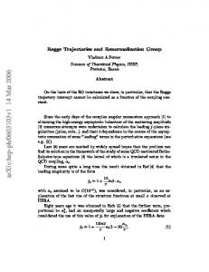
where EN and S2mφ ,nJ (φ, J) can be written as sum of trees defined in the following way.

Fig. 2

v r

v0

h

h+1

N

hv

N +1

Fig 2: an example of tree τ 1) Let us consider the family of all trees which can be constructed by joining a point r, the root, with an ordered set of n ≥ 1 points, the endpoints of the unlabeled tree, so that r is not a branching point. n will be called the order of the unlabeled tree and the branching points will be called the non trivial vertices. The unlabeled trees are partially ordered from the root to the endpoints in the natural way; we shall use the symbol < to denote the partial order. Two unlabeled trees are identified if they can be superposed by a suitable continuous deformation, so that the endpoints with the same index coincide. It is then easy to see that the number of unlabeled trees with n end-points is bounded by 4n . We shall consider also the labeled trees (to be called simply trees in the following); they are defined by associating some labels with the unlabeled trees, as explained in the following items. 2) We associate a label h ≤ N − 1 with the root and we denote Th,n the corresponding set of labeled trees with n endpoints. Moreover, we introduce a family of vertical lines, labeled by an an integer taking values in [h, N + 1], and we represent any tree τ ∈ Th,n so that, if v is an endpoint or a non trivial vertex, it is contained in a vertical line with index hv > h, to be called the scale of v, while the root is on the line with index h. The tree will intersect the vertical lines in set of points different from the root and the end-points; these points will be called trivial vertices. The set of the vertices of τ will be the union of the endpoints, the trivial vertices and the non trivial vertices. Note that, if v1 and v2 are two vertices and v1 < v2 , then hv1 < hv2 . Moreover, there is only one vertex immediately following the root, which will be denoted v0 and can not be an endpoint; its scale is h + 1. There is the constraint, for the end-points of scale hv , that hv = hv0 + 1, if v 0 is the first non trivial vertex immediately preceding v. 3) There R are two kind Rof end-points, normal and special. With each normal endpoint of scale h v we associate zhv −1 dxψ¯x 6 ∂ψx or λ dxdyv(x − y)(ψ¯x γµ ψx )(ψ¯y γµ ψy ) and we call it respectively z or λ end-point. We will P ¯ 4,¯v . There are two types of special call m ¯ 4,v the number of λ end-points with scale hv + 1, and m4,v = v¯≥v m R (1) R dxJµ,x ψ¯x γµ ψx and dx[φ¯x ψx + φx ψ¯x ] endpoints, called of type φ and J and to which is associated Z hv −1

respectively. Given v ∈ τ , we shall call nφv and nJv the number of endpoints of type φ and J following v in the tree. 4) We introduce a field label f to distinguish the field variables appearing in the terms V associated with the endpoints. The set of field labels associated with the endpoint v will be called Iv . Analogously, if v is not an endpoint, we shall call Iv the set of field labels associated with the endpoints following the vertex v; x(f ) will denote the space-time point of the field variable with label f . We call trivial tree a tree containing only the root 19/maggio/2007; 14:57

7

and an endpoint. Defining V (k) (ψ (≤k) , J, φ) = V (k) (ψ (≤k) ) + B (k) (ψ (≤k) , J, φ), we can write 2 V (k) (ψ (≤k) , J, φ) + L4 Ek+1 =

∞ X X

V (k) (τ )

(2.21)

n=1 τ ∈Tk,n

where, if v0 is the first vertex of τ and τ1 , .., τs (s = sv0 ) are the subtrees of τ with root v0 , V¯ (k) is defined inductively by the relation, k ≤ N − 1 V (k) (τ ) =

(−1)s+1 T ¯ (k+1) Ek+1 [V (τ1 ); ..; V¯ (k+1) (τs )] s!

(2.22)

T where Ek+1 is the truncated expectation and V¯ (k+1) (τ ) = RV (k+1) (τ ) if the subtree τi contains more then one end-point, while if τi contains only one end-point V¯ (k+1) (τ ) is equal to (zN = 0) Z Z (≤k+1) (≤k+1) ¯ 6 ∂ψx ; λ dxdyv(x − y)(ψ¯x(≤k+1)) γµ ψx(≤k+1) )(ψ¯y(≤k+1) γµ ψy(≤k+1) ) zk+1 dxψx (1)

if it is a normal end-point, or (ZN = 1) Z (1) Zk+1 dxJµ,x ψ¯x(≤k+1)) γµ ψx(≤k+1)) ;

Z

dx[φ¯x ψx(≤k+1)) + φx ψ¯x(≤k+1)) ]

if it is a special end-point. We will use the following well known representation of the fermionic truncated expectation, see for instance Q (h)ε(f ) [GM], if P is a set of indices and ψ˜(h) (P ) = f ∈P ψx(f ) EhT (ψ˜(h) (P1 ); ψ˜(h) (P2 ); ...; ψ˜(h) (Ps )) =

XY T

l∈T

g (h) (xl − yl )]

Z

dPT (t) det Gh,T (t)

(2.23)

where T is a set of lines forming an anchored tree graph between the clusters of points x(f ) f ∈Pi , that is T is a set of lines, which becomes a tree graph if one identifies all the points in the same cluster. Moreover t = {ti,i0 ∈ [0, 1], 1 ≤ i, i0 ≤ s}, dPT (t) is a probability measure with support on a set of t such that ti,i0 = ui ·ui0 for some family of vectors ui ∈ Rs of unit norm. Finally Gh,T (t) is a (n − s + 1) × (n − s + 1) matrix, whose elements are given by (h) (2.24) (xij − yi0 j 0 ) Gh,T ij,i0 j 0 = ti,i0 g and xij is the one of the points in Pj . In the following we shall use (2.23) even for s = 1, when T is empty, by interpreting the r.h.s. as equal to 1, if |P1 | = 0, otherwise as equal to det Gh = EhT (ψ˜(h) (P1 )). By using (2.21), (2.23) and the definition of the R operation, we get a simple expression for V (h) (τ ), for any τ ∈ Th,n . We associate with any vertex v of the tree a set Pv , the external fields of v. The set Pv includes both the field variables of type ψ which belong to one of the λ, z, J endpoints following v and are not yet contracted at scale hv (in the iterative integration procedure), to be called normal external fields, and those which belong to an endpoint of type λ, z, J and are contracted with a field variable belonging to an endpoint v˜ of type φ through a propagator g (hv˜ −1) , to be called special external fields of v. These subsets must satisfy various constraints. First of all, if v is not an endpoint and v1 , . . . , vsv are the sv vertices immediately following it, then Pv ⊂ ∪i Pvi . We shall denote Qvi the intersection of Pv and Pvi ; this definition implies that Pv = ∪i Qvi . The subsets Pvi \Qvi , whose union will be made, by definition, of the internal fields of v, have to be non empty, if sv > 1, that is if v is a non trivial vertex. Moreover, if the set Pv0 contains only special external fields, that is if |Pv0 | = nφ , and v˜0 is the vertex immediately following v0 , then |Pv0 | < |Pv˜0 |. Given τ ∈ Th,n , there are many possible choices of the subsets Pv , v ∈ τ , compatible with all the constraints; we shall denote Pτ the family of all these choices and P the elements of Pτ . Then we can write, calling 19/maggio/2007; 14:57

8

S Pv0 = Pva0 Pvb0 where Pva0 correspond to the normal external fields and Pvb0 to the special external fields (spinor indices are omitted) V¯ (k) (τ ) =

X X X Z

dxv0 Wτ,P,T,α (xv0 )[

where Y

Wτ,P,T,α (xv0 ) =

v not e.p.

l∈Tv

1

dtl 0

Z

1 0

ψx(f )

f ∈Pva0

P∈Pτ T ∈T α∈AT

hYZ

ε(f )(≤k)

Y

][

Y

ε(f )(≤k)

g (hv˜ −1) (x(f ) − y(f ))φy(f )

1 sv !

Y

J(xf )]

f

f ∈Pvb0

Z

][

(2.25)

dPTv (tv ) · det Ghαv ,Tv (tv )

i Y Y (1) Y − + Z hv ] zhv ][ (r)bα λv(r)][ dsl ∂˜qα (fl ) ∂˜qα (fl ) [(xl (tl )−yl (sl ))bα (l) ∂ ml g (hv ) (xl (tl )−yl (sl ))] [ ∗ v∈vλ

v∈vz∗

∗ v∈vZ

(2.26) and x0 (t), y0 (t) are the interpolated points (see (2.17)) produced in the renormalization, AT is a set of indices necessary to label the terms produced by the R operation, T is the set of the tree graphs on x v0 , obtained by putting together an anchored tree graph Tv for each non trivial vertex v and adding lines connecting the ∗ space-time points belonging to the set xv for each endpoint v; vλ∗ , vz∗ , vZ are the λ, z and Z (1) endpoints of τ , − + hv ,Tv fl and fl are the labels of the two fields forming the line l and Gα (tv ) is the matrix with elements −

+

hv ,Tv qα (fl ) qα (fl ) Gα,ij,i ∂ ∂ 0 j 0 = tv,i,i0 ∂

− m(fi,j )+m(fi+0 ,j 0 ) (hv )

g

(xij − yi0 j 0 ) .

(2.27)

with (fij− , fi+0 j 0 ) not belonging to T . By construction, there is a constant C such that, ∀T ∈ Tτ , |AT | ≤ C n ; moreover, for any α ∈ AT , qα (l) = 0, 1, 2,bα(l) = 0, 1, 2 and by the definition of R the following inequality is satisfied i ih Y h Y Y γ −z(Pv ) , (2.28) γ −hα (l)bα (l) ≤ γ hα (f )qα (f ) v not e.p.

l∈T

f ∈Iv0

where hα (f ) = hv0 −1 if f ∈ Pv0 , otherwise it is the scale of the vertex where the field with label f is contracted; hα (l) = hv , if l ∈ Tv and ( 2 if |Pv | = 2, nφv = 0, 1 nJv = 0 , z(Pv ) = 1 if |Pv | = 2 and nJv = 1, nφv = 0 , (2.29) 0 otherwise. In order to derive (2.25) one has to follow an iterative procedure writing the R operation as in (2.17) and decomposing the ”zero” factors (xµ − zµ ) alongRthe propagators in T and the interactions v(r). Note that, from R (2.6), dr|r||g (h) (r)| ≤ Cγ −2h , and from (2.7), dr|r||v(r)| ≤ Cγ −3N ; hence each zero factor produces an extra γ −h or γ −N ≤ γ −h in the bounds. An important property that one has to check is that the zero factors do not accumulate, that is bα ≤ 3; such procedure has been extensively described in §3 of [BM] to which we refer for more details. We will use now the following bound | det Ghαv ,Tv (tv )| ≤ C γ3

hv 2

(

P sv

i=1

|Pvi |−|Pv |−2(sv −1)) hv

γ

Psv

i=1

P sv

i=1

|Pvi |−|Pv |−2(sv −1)

[qα (Pvi \Qvi )+m(Pvi \Qvi )] γ −hv

P

l∈Tv

[qα (fl+ )+qα (fl− )+m(fl+ )+m(fl− )]

(2.30)

The proof is based on the well known Gram-Hadamard inequality, stating that, if M is a square matrix with elements Mij of the form Mij =< Ai , Bj >, where Ai , Bj are vectors in a Hilbert space with scalar product < ·, · >, then Y | det M | ≤ ||Ai || · ||Bi || . (2.31) i

where || · || is the norm induced by the scalar product. 19/maggio/2007; 14:57

9

Let H = Rs ⊗H0 , where H0 is the Hilbert space of complex four dimensional vectors F (k) = (F1 (k), . . . , F4 (k)), Fi (k) being a function on the set D, with scalar product < F, G >=

4 X 1 X ∗ Fi (k)Gi (k) . L4 i=1

(2.32)

k

If hv ≤ 0, it is easy to verify that (h )

(h )

(h )

v v ,Tv Ghij,i (xij − yi0 j 0 ) =< ui ⊗ Ax(fv − ),ω(f − ) , ui0 ⊗ Bx(fv + 0 j 0 = ti,i0 g − ω ,ω + l

ij

l

i0 j 0

ij

),ω(fi+0 j 0 )

>,

(2.33)

where ui ∈ Rs , i = 1, . . . , s, are the vectors such that ti,i0 = ui · ui0 , and  if ω = 1,  (ik0 + k3 , 0, k1 − ik2 , 0, 0, 0, 0, 0), fh (k)  (0, k1 + ik2 , 0, ik0 − k3 , 0, 0, 0, 0), if ω = 2, (h) ikx · Ax,ω (k) = e (0, 0, 0, 0, ik + k , 0, −k + ik , 0), if ω = 3,  |k| 0 3 1 2  (0, 0, 0, 0, 0, −k1 − ik2 , 0, ik0 + k3 ), if ω = 4,  (1, 1, 0, 0, 0, 0, 0, 0), if ω = 1, p   f (k) (0, 0, 1, 1, 0, 0, 0, 0), if ω = 2. h (h) Bx,ω (k) = eiky · (0, 0, 0, 0, 1, 1, 0, 0), if ω = 3,  |k|  (0, 0, 0, 0, 0, 0, 1, 1), if ω = 4. p

By using (2.26) and (2.30) and | Z Y

v not e.p.



R

(2.34)

(1)

drv(r)| ≤ Cγ −2N and assuming |zk | ≤ C|λ|,|Zk − 1| ≤ C|λ| we find

dxv0 |Wτ,P,T (xv0 )| ≤ L4 γ −h[−4+

3|Pv0 | −2m4,v0 +nJ v0 ] 2

 1 Psv |Pvi |−|Pv | −[−4+ 3|Pv | −2m4,v +nJv +zv ] Y −2N m ¯ 4,v 2 ] [ γ C i=1 γ sv ! v

where for the integration over the interpolated points we proceed as discussed in §3.15 of [BM]. Finally by using the identity Y Y ¯ 4,v γ h2m4,v0 γ (hv −hv0 )2m4,v = γ hv 2m v

(2.35)

(2.36)

v

we finally obtain Z

dxv0 |Wτ,P,T (xv0 )| ≤ L4 γ −h[−4+

3|Pv0 | +nJ v0 ] 2

C n |λ|n¯

Y

v not e.p.



 1 −[−4+ 3|Pv | +nJv +zv ] Y −2(N −hv )m ¯ 4,v 2 [ γ ] γ sv ! v

(2.37)

2.3 Bound for the effective potential We bound the contribution to the effective potential, which is given by 2 ˜k+1 V (k) (ψ (≤k) , J, φ) + L4 E =

∞ X X

n=1

V (k) (τ )

(2.38) ,

∗ τ ∈Tk,n

∗ where Tk,n is the set of trees with nφ = nJ = 0; note that in such a case 4 − 3|P2 v | + zv > 0. Regarding the sum over T , it is empty if sv = 1. If sv > 1 and Nvi ≡ |Pvi | − |Qvi |, the number of anchored trees with di lines branching from the vertex vi can be bounded, by using Caley’s formula, by (see for instance [GM]) (sv − 2)! d N d1 ...Nvssvv ; (d1 − 1)!...(dsv − 1)! v1 19/maggio/2007; 14:57

10

P sv Q P hence the number of addenda in T ∈T is bounded by v not e.p. sv ! C i=1 |Pvi |−|Pv | . In order to bound the sums over the scale labels and P we first use the inequality O(e(κγ −N )θ )

Y

γ −[−4+

3|Pv | +zv ] 2

≤[

Y

1

γ − 40 (hv˜ −hv˜0 ) ][

v ˜

v not e.p.

Y

γ−

|Pv | 40

]

(2.39)

v not e.p.

where v˜ are the non trivial vertices, and v˜0 is the non trivial vertex immediately preceding v˜ or the root. The 1 factors γ − 40 (hv˜ −hv˜0 ) in the r.h.s. of (2.39) allow to bound the sums over the scale labels by C n . Finally the sum over P can be bounded by using the following combinatorial inequality. Let {p v , v ∈ τ } a set P sv of integers such that pv ≤ i=1 pvi for all v ∈ τ which are not endpoints; then Y

X

pv

γ − 40 ≤ C n .

(2.40)

v not e.p. pv

We have finally to show that zh is bounded for any h. By construction zh verifies an equation of the form zh−1 = zh + βz(h) (zh+1 , .., zN , λ)

(2.41)

(h)

and βz (zh+1 , .., zN , λ) is sum of trees with at least one end-point of type λ, as the trees with only z end-points ¯ the scale of are vanishing at zero momenta, for the compact support properties of the propagators. Calling h ¯ a λ end-point, the factor γ −2(N −h) in (2.37) and the fact that 4 − 3|P2 v | + zv > 0 implies that, for a suitable constant θ > 0 |βz(h) (zh+1 , .., zN , λ)| ≤ C|λ|γ 2θ(h−N ) (2.42) and by iteration |zh | ≤

N X

|βz(h) | ≤ C|λ|

(2.43)

k=h (h)

This implies that the kernels W2l of the effective potential verify the bound 1 L4

Z

(h)

dx|W2l (x)| ≤ C l γ −h(−4+3l) |λ|l−1

(2.44)

2.4 Bounds for the correlations 5 We have obtained an expression for hjµ,p ; ψk ψ¯k−p i of the form hjµ,p ; ψk ψ¯k−p i =

∞ N −1 X X

X

X

n=0 j0 =−∞ τ ∈Tj0 ,n (1)

Gτ (p, k) ,

P∈P |Pv0 |=2

(1)

Note first that Zh = 1 + O(λ)), as also the beta function for Zh verifies the bound (2.42). Let us define, for any k 6= 0, hk = min{j : fj (k) 6= 0} and suppose that p, k, p − k are all different from 0. It follows that, given τ , if h− and h+ are the scale indices of the ψ fields belonging to the endpoints associated with φ+ and φ− , while hJ denotes the scale of the endpoint of type J, G2,1 τ (p, k) can be different from 0 only if h− = hk , hk + 1, h+ = hk−p , hk−p + 1 and hJ ≥ hp − logγ 2. Moreover, if Tj0 ,n,p,k R denotes the set of trees satisfying the previous conditions and τ ∈ Tj0 ,n,p,k , |Gτ (p, k)| can be bounded by dzdx|Gτ (z; x, y)|. Hence we get, if dv = −4 + 3|P2 v | + nJv + zv |hjµ,p ; ψk ψ¯k−p i| ≤ Cγ −hk γ −hk−p

∞ N −1 X X

X

n=0 j0 =h−1 τ ∈Tj0 ,n,p,k

19/maggio/2007; 14:57

11

X

P∈P |Pv0 |=2

(C|λ|)n

Y

v not e.p.

γ −dv .

(2.45)

Given τ ∈ Tj0 ,n,p,k , let v0∗ the higher vertex preceding all three special endpoints and v1∗ ≥ v0∗ the higher vertex preceding either the two endpoints of type φ (to be called vφ,+ and vφ,− ) or one endpoint of type φ and the endpoint of type J (to be called vJ ). It turns out that dv > 0, except for the vertices belonging to the path C ∗ connecting v1∗ with v0∗ , where, if |Pv | = 2 and nJv = 1, dv = 0. Hence, we can sum over the scale and Pv labels of ∗ ∗ τ , only if we fix the scale indices h∗0 and h∗1 of v0∗ and v1∗ , after multiplying by γ −δ(h1 −h0 ) , δ being any positive ∗ ∗ number. Of course, we have also to perform the sum over h∗0 , h∗1 of γ δ(h1 −h0 ) , which is divergent, if we proceed exactly in this way. In order to solve this problem, we note that, if v ∈ / C ∗ , dv − 1/4 > 0. Hence, before performing the sums over −dv the scale and Pv labels, we can extract from each γ factor associated with the vertices belonging to the paths connecting the three special endpoints with v0∗ or v1∗ , a γ −1/4 piece, to be used to perform safely the sums over h∗0 , h∗1 in the following way. (1) Let us consider first the family Tj0 ,n,p,k of trees such that the two special endpoints following v1∗ are vφ,+ and vφ,− and let us suppose that |k| ≥ |k − p|. In this case, before doing the sums over the the scale and P v labels, we fix also the scale hJ of vJ . We get, if h∗J ≡ max{hp + 2, h∗0 + 1}, if dv = −4 + 3|P2 v | + nJv + zv : ∞ N −1 X X

n=0 j0 =h−1 ∗

hk−p

h1 X

X

≤C

X

X

∗

∗

γ −dv ≤

v not e.p.

P∈P (1) τ ∈Tj ,n,p,k |Pv |=2 0 0

+∞ X

Y

(C|λ|)n

∗

1

∗

∗

γ δ(h1 −h0 ) γ − 4 [(hk −h1 )+(hk−p −h1 )+(hJ −h0 )]

(2.46)

∗ ∗ h∗ 1 =−∞ h0 =−∞ hJ =hJ

and the r.h.s. can be bounded by, multiplying and dividing by γ δ(hk −hp ) ∗

hk−p 0 δ(hk −hp )

Cγ

X

γ

h1 X

∗ ∗ 1 δ(h∗ 1 −hk ) − 4 [(hk −h1 )+(hk−p −h1 )

γ

h∗ 1 =−∞

∗

1

∗

∗

γ δ(hp −h0 ) γ − 4 (hJ −h0 )

(2.47)

h∗ 0 =−∞

so that the r.h.s. of (2.47) is bounded by Cγ δ(hk −hp ) , if δ ≤ 1/8. If |k − p| ≥ |k|, we get a similar result, with hk−p in place of hk . (2,+) Let us consider now the family Tj0 ,n,p,k of trees such that the two special endpoints following v1∗ are vJ and ∗ ¯ 0 = min{hk−p, h∗ }: vφ,+ . We get, if hJ ≡ max{hp + 2, h∗1 + 1} and h 1 ∞ N −1 X X

X

n=0 j0 =h−1 τ ∈T (1,+)

≤C

hk X

¯

h0 X

X

(C|λ|)n

∗

∗

γ −dv ≤

v not e.p.

P∈P j0 ,n,p,k |Pv0 |=2

+∞ X

Y

1

∗

∗

∗

γ δ(h1 −h0 ) γ − 4 [(hk −h1 )+(hk−p −h0 )+(hJ −h1 )]

(2.48)

∗ ∗ h∗ 1 =−∞ h0 =−∞ hJ =hJ

and it is easy to prove that, if δ ≤ 1/8, the r.h.s. of (2.48) is bounded by Cγ δ(hk −hk−p ) , if |k| ≥ |k − p|, by a (2,−) constant, otherwise. The family Tj0 ,n,p,k of trees such that the two special endpoints following v1∗ are vJ and vφ,− can be treated in a similar way and one obtains a bound Cγ δ(hk−p −hk ) , if |k − p| ≥ |k|, or a constant, otherwise. By putting together all these bounds, we get, for any positive δ ≤ 1/8: |hjµ,p ; ψk ψ¯k−p i| ≤

 δ  δ  δ  δ |k| |k − p| |k| |k − p| Cδ [ + + + ] |k||k − p| |p| |p| |k − p| |k|

(2.49)

with Cδ → ∞ as δ → 0. Note that the contributions from all trees with at least a λ end-point admit a similar bound with an extra Q ¯ 4,v in (2.37). This means that the only non vanishing γ −θ(N −hk ) , for the presence of the factor v γ −2(N −hv )m 19/maggio/2007; 14:57

12

trees, at fixed k, p and in the limit N → ∞, are the ones with one Z (1) end-point and any number of Z endpoints; the corresponding Feynman graphs are chain graphs. For similar reasons, only trees with no λ end-points contribute in the limit N → ∞ at finite k to hψk ψ¯k i.

3. Ward Identities 3.1 Ward Identities with cut-offs With the transformations ψ¯x → ψ¯x e−iαx

ψx → eiαx ψx the generating function becomes Z R eWN,L (J,φ) = P (dψ (≤N ) )e−

(3.1)

¯x (eiαx D (≤N ) e−iαx −D (≤N ) )ψ − −V +( dxψ x

e

R

¯x e−iαx +e−iαx φ ¯x ψx ] dx[φx ψ

(3.2)

P ε (k)i 6 kψk . In deriving the above expression we have used that that the where D(≤N ) ψx = L14 k e−ikx CN Jabobian corresponding to the transformation (3.1) is 1; in fact Z

Dψ[

Y

x∈A+

ψ¯x ][

Y

y∈A−

ψy ] =

1 L4|A+ |

X

e

k1 ...k|A+ |

i

P|A+ | i=1

ki xi

1 L4|A− |

X

p1 ...p|A− |

e

−i

P|A− | i=1

p i yi

Z

|A− |

|A+ |

Dψ[

Y

i=1

ψ¯ki ][

Y

ψpi ]

i=1

(3.3) By definition of Grassman variables the only nonvanishing term in the sum in the r.h.s. correspond to an addend + A− with all the k, p distinct; moreover one can have a nonvanishing term only if {ki }A i=1 = {pi }i=1 = D, and this + − A is possible only if the xi , yi are all different and such that {xi }A i=1 = {yi }i=1 = Λa , so that Z Z Y Y Y Y Y ψ¯x ][ Dψ[ ψy ] = Dψ [ eiαx ψ¯ω,x ][ e−iαx ψx ] (3.4) x∈A+

ω x∈A+

y∈A−

x∈A−

We use write the exponent of (3.2) as Z Z Z (≤N ) (≤N ) (≤N ) ¯ (≤N ) ¯ ¯ ¯ dx[ψx D (αx ψx )−αx ψx D ψx ] = dxαx [(D ψx )ψx + ψx (D ψx )] = dxαx [6 ∂(ψ¯x ψx )+αx δjx ] (3.5)

where δjx =

1 X i(k+ −k− )x e C(k+ , k− )ψ¯k+ ψk− L8 + −

(3.6)

k 6=k

and −1 + − C(k+ , k− ) = (χ−1 N (k ) − 1)i 6 k− − (χN (k ) − 1)i 6 k+

(3.7)

Differentiating with respect to αx both sides of (3.2), and setting αx = 0 we find and finally making a derivative with respect to φx , φy and passing to Fourier transform − + − −ipµ hjpµ ; ψ¯k+p ψ¯L,k iN,L = hψ¯k+ ψk− iN,L − hψ¯k+p ψk+p iN,L − hδjp ; ψ¯k+p ψk iN,L

(3.8)

By comparing (3.8) with (1.4), we see that they differ form the presence of the last term in (3.8), which take into account of the presence of the ultraviolet cut-off and it is indeed of the same order of magnitude of the other correlations in (3.8). We will prove in the following section the following identity hδjp ; ψ¯k+p ψk iN,L = −νN hjp ; ψ¯k+p ψk iN,L + RN,L(p; k)

(3.9)

where νN = −i 6 p(c+ e2 + O(e4 )), for a suitable constant c+ and RN (k, p) is a small correction, as it verifies the − same bound as pµ hjpµ ; ψ¯k+p ψ¯L,k i up to an extra factor γ −θ(N −hk) , if hk is the scale of k. In order to do this we write RN,L (p, k) as ∂3 ˆ N,L |J=φ=φ=0 RN,L (p; k) = W ¯ ∂Jp ∂φk ∂ φ¯k−p 19/maggio/2007; 14:57

13

ˆ

eWN,L (J,φ) =

Z

P (dψ (≤N ) )e

−V (N ) (ψ)+ L14

P

p∈D

Jp χ ¯N (p)δjp +νN

P

1 L4

p∈D

µ Jp pµ jp + L14

P

k∈D

¯k +ψ ¯k φk ] [ψk φ

(3.10)

ˆ N,L is analyzed by a multiscale integration similar to the one on §2: note that we can freely multiply δj p and W by a smooth compact support function χ(p), ¯ equal to 1 for |p| ≤ 3γ N and 0 for |p| ≥ 4γ N , as by the compact support properties of the propagators the values of p are such that χ(p) ¯ = 1. 5 5 In the massless case, by the change of variables ψx → eiγ αx ψx ψ¯x → ψ¯x e−iγ αx and proceeding in the same way we get − + − 5 −ipµ hjµ,p ; ψ¯k+p ψ¯L,k iN,L = hψ¯k+ ψk− iN,L − hψ¯k+p ψk+p iN,L − hδjp5 ; ψ¯k+p ψk iN,L

(3.11)

and also in such case a decomposition like (3.9) holds; in the following we will prove (3.9), but all the computations can be repeated in the case (3.10) up to some obvious modifications. 3.2 Analysis of the corrections ˆ N,L(J, φ) following a multiscale procedure writing We integrate W Z Z P P P µ ¯k +ψ ¯k φk ] ˆ −V (N ) (ψ)+ L14 Jp δjp +νN L14 Jp pµ jp + L14 [ψk φ p∈D p∈D k∈D eWN,L (J,φ) = P (dψ (≤N −1) ) P (dψ (N ) )e

(3.12)

and integrating iteratively the fields ψ (N ) , ψ (N −1) ..., ψ (h) . In the expansion for RN,L(p, k) the following quantity will appear ∆h,k (k+ , k− ) = g (h) (k+ )C µ (k+ , k− )g (k) (k− ) = χ(p) ¯

fh (k+ ) fk (k− ) fk (k− ) fh (k+ ) − [ − f (k )] − [ − fh (k+ )] k i 6 k+ χN (k− ) i 6 k− χN (k+ ) (3.13)

such that ∆h,k (k+ , k− ) = 0

h, k < N

(3.14)

(h)

as χN (k) = 1 in the support of g (k) when h ≤ N − 1. Moreover for j ≤ N − 1 we can write ∆

N,j

fj (k− )uN (k+ ) fj (k− ) (k , k ) = −χ(p) = −χ(p) pµ i 6 k− i 6 k− +

−

Z

1 0

dt∂µ uN (k+ + tp) ≡ pµ SµN,j (k+ , k− )

where uN (k) = 0 for |k| ≤ γ N and uN (k) = 1 − fN (k) for |k| ≥ γ N ; in fact fN (k) χN (k)

fj (k) χN (k)

− fj (k) = 0 for j ≤ N − 1 and

N

− fN (k) ≡ uN (k) is vanishing for |k| ≤ γ and it is equal to 1 − fN (k) for |k| ≥ γ N . A similar expression can be written for ∆j,N , using that ∆h,k is symmetric. The Fourier transform Z Sµ(N,j) (x − y, x − z) = dk+ dk− e−i(k+ −k− )x eik+ y e−ik− z S (N,j) (k+ , k− ) (3.15) verifies the bound |SµN,j (z − x, z − y)| ≤ Cn

γ 3j γ 3N 1 + [γ N |z − x|]n 1 + [γ j |z − y|]n

(3.16)

The bound follows integrating by parts, noting that volume factors are γ 4j (for the support of fj ) and γ 4N (for + −j the support of χ(p)u ¯ while each derivative N (k )), and each derivative with respect to k− gives and extra γ −N with respect to k+ gives an extra γ . In the same way Z Z fj (k+ ) 1 fN (k− ) 1 dt∂µ uN (k+ + tp) − dt∂µ uN (k− + tp)] ∆N,N (k+ , k− ) = χ(p)pµ [ 6 k− 6 k+ 0 0 After the integration of ψ N in (3.12) we get e 19/maggio/2007; 14:57

ˆ N,L (J,φ) W

=e

ˆN (φ,J) −L4 EN +S

Z

P (dψ (≤N −1) )e−V 14

(N −1)

(ψ (≤N −1) )+B(N −1) (ψ,J,φ)

(3.17)

where V (N −1) is the same as in (2.9) and B (N −1) can be again decomposed as in (2.12); we can write (N −1)

B1

a(N −1)

(ψ (≤N −1) , J) = B1

b(N −1)

(ψ (≤N −1) , J) + B1

(ψ (≤N −1) , J)

(3.18)

P a(N −1) (ψ (≤N −1) , J) (ψ (≤N −1) , J) is obtained from the contraction of νN L14 p∈D Jp pµ jµ,p and B1 P (N −1) and is obtained from the contraction of L14 p∈D Jp δjp . The L operation is defined as in §2 for V (N −1) , B2 b(N −1)

where B1 (N −1)

B3

. We can write

b(N −1)

B1

=

∞ 2l X X Y 1 X 1 X 1 X (N −1) ... p W (p, k)J(p)δ(p ε k ) ψkεii + µ i i µ,2l L4 p L4 L4 i i=2 l=2

k1

and we define L = 0 for l > 1 and

k2l

(N −1)

LWµ,2 (N −1)

and again by symmetry Wµ,2

(N −1)

(p, k) = Wµ,2

(0, 0)

(3.19)

(0, 0) = γµ Z where Z is a constant. a(N −1)

Finally we define L = 0 for all the terms in B1 with more than two fermionic fields; the terms with two fields can be written as 1 X 1 X¯ 1 X N,N ˜ ˜ ˜ k, k − p)+ Jp p µ 4 Sµ (k, k − p)G4 (k, (3.20) ψk ψk+p { 4 4 L p L L ˜ k

k

[(χN (k)−1 − 1)i 6 kg (N ) (k + p) − uN (k + p)]G2 (k + p) + [(χN (k + p)−1 − 1)(i 6 k + i 6 p)g (N ) (k) − uN (k)]G2 (k)} where we distinguish the terms obtained from the contraction of δj are such that or the two fields in δj or one field are contracted; the case corresponding the two fields non contracted is absent thanks to (3.14). We can replace G2 (k) in (3.20) with G2 (k) − G2 (0), using that, by parity, G2 (0) = 0; this improve the bound 0 of a factor γ −N +h , where h0 is the scale at which one of the external ψ fields are contracted. Finally we define the L operation over the first addend of (3.20) as L

1 X N,N ˜ ˜ 1 X¯ 1 X ˜ ψ ψ [ J p Sµ (k, k − p)GN k k+p p µ 4 (k, k, k − p)] = L4 p L4 L4 ˜ k

k

1 X¯ 1 X 1 X N,N ˜ ˜ ˜ 0, 0)] Jp p µ 4 Sµ (k, k)G4 (k, ψk ψk+p [ 4 4 L p L L

(3.21)

˜ k

k

By Euclidean invariance we find (N −1) LB1 (ψ (≤N −1) , J)

= νN −1

Z

dxψ¯x 6 ∂ψx

(3.22) (h)

The procedure can be iterated integrating the fields ψ N −1 , ψ N −2 , ..ψ h ; we can still decompose B1 R b(h) b(h) B2 where B2 is obtained from the contraction of νk dxψ¯x 6 ∂ψx for some k ≥ h and a(h)

B1

=

1 X 1 X¯ 1 X N,h ˜ ˜ ˜ k ˜ − p)]Gh (k, ˜ k, k − p)] Jp p µ 4 ψk ψk+p [ 4 [Sµ (k, k − p) + Sµh,N (k, 4 4 L p L L k

a(h)

as B1

+

(3.23)

˜ k

and the L operation is defined as before. Assume now that |νh | ≤ c0 |λ|γ θ(h−N ) ,

(3.24)

We have obtained an expression for RN,L (3.10) of the form RN,L (p; k) =

∞ N −1 X X

X

n=0 j0 =−∞ τ ∈Tj0 ,n,2,1

19/maggio/2007; 14:57

15

X

P∈P |Pv0 |=2

Rτ (p, k) ,

and the trees are defined as before, with the only important difference that there are endpoints v to which is P P associated νhv L14 p∈D Jp pµ jµ,p or, if hv = N , L14 p∈D Jp δjµ,p : in both case we have the constraint that hv −hv0 = 1, if v 0 is the first non trivial vertex following v. We call such end-points of type Tν and T0 respectively. The sum over the trees such that the endpoint is of type Tν can be bounded as in (2.45), the only difference being that, thanks to the bound (3.24), one has to multiply the r.h.s. by a factor |λ|γ −θ(N −hJ ) , which has to be inserted also in the r.h.s. of the bounds (2.46) and (2.48). Hence the analogous of the r.h.s. of (2.46) becomes ∗

hk−p

h1 X

X

+∞ X

∗

∗

∗

1

∗

∗

γ δ(h1 −h0 ) γ − 4 [(hk −h1 )+(hk−p −h1 )+(hJ −h0 )] γ −θ(N −hJ )

(3.25)

∗ ∗ h∗ 1 =−∞ h0 =−∞ hJ =hJ

and the r.h.s. can be bounded by, multiplying and dividing by γ δ(hk −hp ) ∗

hk−p 0 δ(hk −hp )

Cγ

X

γ

∗ ∗ 1 δ(h∗ 1 −hk ) − 4 [(hk −h1 )+(hk−p −h1 )]

γ

h∗ 1 =−∞

h1 X

∗

∗

1

∗

∗

γ δ(hp −h0 ) γ − 4 (hJ −h0 ) γ −θ(N −hJ )

(3.26)

h∗ 0 =−∞

so that the r.h.s. of (2.47) is bounded by Cγ δ(hk −hp ) (γ −N κ)θ , if δ ≤ 1/8 and |p|, |k − p|, |k| ≤ κ; in fact ∗ ∗ ∗ ∗ γ hJ = γ hp +2 if hp ≥ h∗0 − 1 and γ hJ = γ h0 +1 ≤ γ h1 +1 ≤ γ hk−p +1 if hp < h∗0 − 1. In a similar way also the other cases have an extra factor (γ −N κ)θ . Let us now consider the trees with an endpoint of type T0 ; in such case the fields of the T0 endpoint are contracted at scale j, N ; this implies that the sum over hJ is missing in the r.h.s. of the bounds (2.46) and (2.48) and hJ = N ; the analogous of (2.46) becomes then hk−p

X

∗

h1 X

∗

∗

∗

1

∗

∗

γ δ(h1 −h0 ) γ − 4 [(hk −h1 )+(hk−p −h1 )+(N −h0 )]

(3.27)

∗ h∗ 1 =−∞ h0 =−∞ ∗

and γ −(N −h0 ) ≤ γ −(N −hk−p ) so that again there is an improvement in the bounds of a factor (γ −N κ)θ . Hence RN,L (p; k) verifies a bound similar to (2.49), with an extra factor (γ −N κ)θ . 3.3 The flow of the counterterms We have finally to prove (3.24). The flow equation has the form νj−1 = νj + βν(j) (νj ; . . . ; νj ; λ) , and βν(j) (νj ; . . . ; νN ; λ) = βν(j,1) (λ) +

N X

(3.28)

0

νj 0 β˜ν(j,j ) (λ) .

(3.29)

j 0 =j

Moreover given a positive θ < 1/4, there are constants c1 and c2 such that |βν(j,1) (λ)| ≤ c1 |λ|γ 2θ(j−N )

0

0

|β˜ν(j,j ) (λ)| ≤ c2 λ2 γ 2θ(j−j ) .

,

(3.30)

0

(j,1) (j,j ) This follows from the fact that βν and β˜ν are given by a sum of trees verifying the bound (3.31) , with at least an end-point respectively at scale N and at scale j 0 , hence one can improve the bound respectively by a 0 factor γ 2θj and γ 2θ(j−j ) . By a simple iteration, (3.28) can also be written in the form

νj−1 = νN +

N X

0

βν(j ) (νj 0 ; . . . ; νN ; λ) .

j 0 =j 19/maggio/2007; 14:57

16

(3.32)

By choosing νN = −

N X

βν(j) (νj,ω ; . . . ; νN ; λ) ,

(3.33)

j=−∞

we see, by inserting (3.33) in the r.h.s. of (3.32), that we have to show that there is a sequence ν = {ν j , j ≤ N }, such that νN is of order λ and j X 0 νj = − (3.34) βν(j ) (νj 0 , .., νN ; λ) . j 0 =−∞

¯ h γ θj , In order to prove that, we introduce the space Mθ of the sequences ν = {νj , j ≤ N } such that |νj | ≤ cλ −θ(j−N ) −1 |λ| . We then look for some c; we shall think Mθ as a Banach space with norm ||ν||θ = sup≤j≤N |νj |γ for a fixed point of the operator T : Mθ → Mθ defined as: j X

(Tν)j = −

0

βν(j ) (νj 0 , .., νN ; λ) .

(3.35)

j 0 =−∞

Note that, if λ is sufficiently small, then T leaves invariant the ball Bθ of radius c0 = 2c1 c1 being the constant in (3.30). In fact, by (3.29) and (3.30), if ||ν||θ ≤ c0 , then |(Tν)j | ≤

j X

0

c1 |λ|γ 2θj +

j 0 =−∞

P∞ if 2c2 |λ|( n=0 γ −n )2 ≤ 1. T is a also a contraction on

j 0 X X

j 0 =−∞

c0 |λ|γ θ(i−N ) c2 λ2 γ 2θ(j

0

−i)

P∞

n=0

γ −n of

≤ c0 |λ|γ θ(j−N ) ,

j X

0

0

0 |βν(j ) (νj 0 , .., νN ; λ) − βν(j ) (n0j 0 , .., νN ; λ)|

j 0 =−∞

≤

0 X

0

||ν − ν ||θ |λ|γ

(3.37) θ(i−N )

2 2θ(j 0 −i)

c2 λ γ

j 0 =−∞ i=j 0

if c2 λ2 (

P∞

n=0

(3.36)

i=j 0

Bθ , if λ is sufficiently small; in fact, if ν, ν 0 ∈ Mθ ,

|(Tν)j − (Tν 0 )j | ≤ j X

Mθ ,

1 ≤ ||ν − ν 0 ||θ |λ|γ θ(j−N ) , 2

γ −n )2 ≤ 1/2. Hence, by the contraction principle, there is a unique fixed point ν ∗ of T on

Bθ .

4. Appendix 1: Computation of c+

The value of ν at lowest order is obtained from the localization of the following terms Z dk0 χN (k0 ) χN (k0 + p) I1 + I2 = v(p) Tr[γν CN (k0 , k0 + p) ]γν + 4 0 (2π) i6k i(6 k0 + 6 p) Z dk0 χN (k0 ) χN (k0 + p) 0 0 0 v(k )[γ C (k , k + p) γν ] ν N (2π)4 i 6 k0 i(6 k0 + 6 p)

(4.1)

Using that g (≤N ) (k)CN (k, k + p)g (≤N ) (k + p) = (1 − χN (k))χN (k + p)[

1 1 1 − ] + (χN (k) − χN (k + p)) (4.2) i(6 k+ 6 p) i 6 k i6k

we find that LI1 = v(p)pα

Z

19/maggio/2007; 14:57

dk ∂ kµ (1 − χN (k))χN (k) Tr(γν γµ )γν − v(p)pα (2π)4 ∂kα ik2 17

Z

dk ∂ kµ [ χN (k)] 2 Tr(γν γµ )γν (2π)4 ∂kα ik (4.3)

and using that Tr(γν γµ ) = δν,µ and LI1 = −iv(p)pµ In the same way Z LI2 = pα

R

dkkα kβ F (|k|) is vanishing unless ν = α we find

dk ∂ kµ (1 − χN (k))χN (k) γµ + iv(p)pµ (2π)4 ∂kµ k2

Z

dk ∂ kµ v(k)(1 − χ(k))χ(k) γν γµ γν − p α 4 (2π) ∂kα ik2

Z

Z

dk ∂ kµ [ χN (k)] 2 γµ ≡ −i 6 pc1 (2π)4 ∂kµ k

(4.4)

dk ∂ kµ v(k)[ χ(k)] 2 γν γµ γν 4 (2π) ∂kα ik

(4.5)

χ0 (k) dk v(k) 6 p ≡ −i 6 pc2 (2π)4 |k|

(4.6)

which can be rewritten as,using that γν γµ γν = 2γµ LI2 = −i2pµ

Z

∂ kµ µ dk v(k)(1 − χN (k))χN (k) γ + 2i (2π)4 ∂kµ k2

Z

We will call c+ = c1 + c2 .

5. Appendix 2: The WI at lowest orders It is possible to check at lowest order the WI (1.12) by perturbation theory, using the identity χN (k) χN (k + p) χN (k) χN (k + p) χN (k) χN (k + p) − = i6p + CN (k, k + p) i6k i6k+p i6k i6k+i6p i6k i(6 k+ 6 p)

(5.1)

(1) replacing (1.4) when a momentum cut-off is present. Calling hψk ψ¯k i = g(k)Σ(1) g(k) the first order term of the perturbative expansion of the 2-point function, we obtain

[(Σ(1) (k) − Σ(1) (k + p)]|k=0 = −

=−

Z

Z

dk0 χN (k0 ) 0 v(k )[γ γν ] + ν (2π)4 i 6 k0

dk0 χN (k0 ) χN (k0 + p) 0 v(k )[γ i 6 p γν ] + ν (2π)4 i 6 k0 i(6 k0 + 6 p)

Z

Z

dk0 χN (k0 + p) 0 v(k )[γ γν ] ν (2π)4 i(6 k0 + 6 p)

χN (k0 ) χN (k0 + p) dk0 0 0 0 v(k )[γ C (k , k + p) γν ] (5.2) ν N (2π)4 i 6 k0 i(6 k0 + 6 p)

(1) (1) and calling hjpµ ; ψ¯k+p ψ¯k− i = g(k)g(k + p)Γµ (k, p) the first order contribution to hjpµ ; ψ¯k+p ψ¯k− i we obtain

pµ Γ(1) µ (k, p) =

Z

χN (k0 ) χN (k0 + p) dk0 γν ] + v(p) v(k0 )[γν 6p 4 (2π) i 6 k0 i(6 k0 + 6 p)

Z

dk0 χN (k0 ) χN (k0 + p) ]γν (5.3) Tr[γν 6p 4 (2π) i 6 k0 i(6 k0 + 6 p) 0

and the second term, the renormalization of the photon mass, is equal , using (5.1), to iTr[γ ν χNi6k(k0 ) CN (k0 , k0 + 0

N (k +p) p) χi(6 k0 +6p) ]γν . Hence we obtain

(1) (1) (1) −ipµ hjpµ ; ψ¯k+p ψ¯k− i − hψk ψ¯k i + hψk+p ψ¯k+p i =

Z

dk0 χN (k0 ) χN (k0 + p) v(k0 )[γν CN (k0 , k0 + p) γν ] + v(p) 4 0 (2π) i6k i(6 k0 + 6 p)

Z

(5.4)

dk0 χN (k0 ) χN (k0 + p) Tr[γν CN (k0 , k0 + p) ]γν ] 4 0 (2π) i6k i(6 k0 + 6 p)

and the last addend is equal to, up to terms vanishing as N → ∞, to −c+ 6 pµ , in agreement with (1.12).

References [B]

Becchi C. Lectures on the renormalization of Gauge Theories, in Relativity, groups and topology (Les Houches 1983) Eds. B.S. DeWitt and R.Stora (Elsevier Science 1984) [BFM] Benfatto G., Falco P, Mastropietro V.: Comm. Math. Phys., 2007 [BM] Benfatto G., Mastropietro V.: Rev. Math. Phys., 13, 1323–1435, 2001 19/maggio/2007; 14:57

18

[BM1] Benfatto G., Mastropietro V.: Comm. Math. Phys., 231, 97–134, 2002.;Comm. Math. Phys., 258, 609–655, 2005. [BAM] Bonini,M, D’Attanasio, M, Marchesini G. Nucl. Phys. 418, 81, 1994. [DH] Dimock J., Hurd T.L.: J. Math. Phys. 33, 2, 814-821, 1992. [FHRS] Feldman J., Hurd T.L.,Rosen L.,Wrigth,J. QED: a proof of renormalizability. Springer 1988 [G] G.Gallavotti. Rev. Mod.Phys. 55, 471, (1985) [GM] Gentile G, Mastropietro V.: Phys Rep 352, 4-6, 273-343 (2001) [H] Hurd T.R.: Comm. Math. Phys., 125, 515–526, 1989. [IZ] Itzykson,C, Zuber, J. Quantum Field Theory. McGrove-Hill 1985 [KK1] Keller,G,Kopper C: Phys. Lett., 176,B,273 323–332, 1991. [KK] Keller,G,Kopper C: Comm. Math. Phys., 176, 193–226, 1996. [M] Mastropietro V.: J. Math. Phys.,48, 022302 (2007) [P] Polchinski,J. Nucl. Phys. B 231 , 269 (1984) [T] Takahashi,T. Nuovo Cimento 10,6 , 370 (1957) [W] Ward J.C. Phys.Rev. 78 , 182 (1950)

19/maggio/2007; 14:57

19