erative peer-to-peer communication between the mobile users in the form of .... is equipped with an Atheros IEEE 802.11 a/b/g card which we primarily use in the ...
1
Repeatable and Realistic Experimentation in Mobile Wireless Networks Vincent Lenders, Member, IEEE, and Margaret Martonosi, Senior Member, IEEE
✦
Abstract—Experimenting with mobile and wireless networks is challenging because testbeds lack repeatability and existing simulation models are unrealistic for real-world settings. We present practical models for the physical and MAC-layer behavior in mobile wireless networks in order to address this challenge. Our models use measurements of a real network rather than abstract radio propagation and mobility models as the basis for accuracy in complex environments. We develop an adaptive measurement technique in order to maximize the accuracy of our models in dynamic environments. The models then predict the packet delivery, deferring, and collision probability in the same network for an arbitrary set of transmitters. This allows to explore the performance of different network and higher-layer protocols in simulation or emulation under identical and realistic conditions. We evaluate the accuracy of our models empirically by comparing them to benchmark measurements. We find that our models are effective at reproducing mobile scenarios in various environments. Across many experiments in realistic environments, we are able to reproduce link delivery probabilities with RMS error below 12%, and the simulated throughput of data flows in the presence of interfering transmitters with an error that is below 10%. Index Terms—Wireless experiments, measurements, simulation, mobility.
1
I NTRODUCTION
Wireless networks have enjoyed a high popularity in recent years, and the adoption rate continues to grow rapidly in the mobile device market. Wireless networks have traditionally been used in combination with a fixed infrastructure to provide wireless connectivity to nomadic users at ”hotspots”. However, more recent developments have proposed to incorporate cooperative peer-to-peer communication between the mobile users in the form of wireless ad hoc networks. The latter has led to a large effort by researchers to develop new MAC, routing and transport protocols that are able to cope with the dynamic nature of these networks. A large portion of these efforts is concerned with the challenging task of evaluating different protocol design tradeoffs in a systematic and representative way. The two main techniques that have been used for this purpose are field experiments that test real systems in real-world environments and simulation (or emulation) studies that use abstract models to model the wireless network behavior in a synthetic environment. Both techniques have unique benefits but have also inherent limitations. On the one hand, field experiments with real hardware and software allow for a high degree of realism and credibility.
However, this approach faces serious issues in terms of repeatability and control: the radio conditions are almost impossible to reproduce, due to the mobility of the communicating nodes, the variability of radio sources, and the interference of physical objects. Even repeating the same experiment twice under ideal conditions can be a daunting task as we will show in Section 3. In addition, field trials lack a crucial benefit of simulations. It is simply too time-consuming to run experiments in a wide variety of settings. For these reasons, many researchers have understandably embraced simulations. Simulations solve the problems of repeatability and configurability. However, simulations that rely on abstract models found in the literature are often simple, assuming for example that signal propagation is a simple function of distance, that coverage of radios are circular, that interference is twice the transmission range, or that node mobility follows uniform random patterns. As a result, evaluations with wireless simulation tools that rely on such models like ns-2 [1], GloMoSim [19], OMNet++ [2], TOSSIM [13] have been shown to produce results that differ significantly from the reality [11], [12]. In our work, we follow another approach that aims at combining the strengths of both methods by developing models that are seeded by measurements taken in field experiments. Radio propagation and in particular node mobility are sufficiently complex in realistic settings that the only feasible method to model them accurately is by means of physical measurements. Our main goal is therefore to use simple realworld measurements on a mobile network to capture the radio characteristics over time, and then predict how such a network, or part of it, will perform when running under different workloads in a simulator. This allows us to compare different protocols under identical real-world conditions. The methodology we developed works as follows. We use measurements on a network to get channel characteristics between wireless nodes. During the whole measurement phase, each node sends broadcast packets at a constant rate and records all packets that it receives from the other nodes. The broadcasting rate is limited at each node depending on the number of neighbors in order to minimize packet losses caused by interfering transmissions. We then formulate a physical layer model for the packet delivery probability based on the measured broadcast packets that captures the effects of radio propagation, environmental noise, and node mobility. On top of that, a MAC-layer model predicts packet delivery
2
2
E XPERIMENTAL S ETUP
The work described in this paper uses measurements (i) to gain an understanding of wireless characteristics under node mobility, (ii) as input for our models, and (iii) to evaluate the accuracy of our models. The measurement platforms and environment in which we conduct our experiments are described in this section. We use laptops as mobile nodes in our testbed. Each laptop is equipped with an Atheros IEEE 802.11 a/b/g card which we primarily use in the 2.4 GHz frequency band. In all experiments, the wireless cards are operated in ad hoc mode on the same channel. While all experiments are conducted with IEEE 802.11, we expect the presented results to hold in general for CSMA/CA systems. We perform experiments in three different environments to understand the limitations of our models and the effects in different settings: • IN-PED: These experiments consist of indoor measurements where the mobile nodes are carried by people inside a structured building with multiple floors. The nodes are moving at typical pedestrian speed. • OUT-PED: These experiments are conducted outdoors on sunny and dry days. The outdoor environment is flat and relatively free of obstacles such that the mobile nodes almost always have line-of-sight contact. The mobile nodes are carried by people moving at typical walking speeds. • OUT-CAR: In these experiments, a mobile node is mounted inside a car driving on a street at varying speeds with a maximum of 50 km/h. The mobile node inside the car communicates with fixed nodes along the street.
1 delivery probability
under the influence of carrier sense and interference caused by simultaneous transmissions. Our models are effective for exploring the performance of network or higher-level protocols under repeatable and realistic conditions in various settings, i.e., we are able to explore arbitrary communication patterns among an arbitrary subset of the nodes participating in the measurements. We have evaluated our models for the base case in which IEEE 802.11 mobile nodes compete for the same channel in various environments and mobility patterns. We find that our models are accurate at estimating the link delivery probability and the link throughput for many different experiments. Across various settings, the root mean square error (RMSE) of the estimated versus measured benchmark packet probability ranges between 4% and 12%. Furthermore, the error of the estimated throughput versus the effective observed throughput is below 10%, in contrast to up to > 50% for a naive model that ignores carrier sense and interference effects. The rest of this paper is structured as follows. In the next section, we introduce the experimental setup we base our measurements on. In section 3, we review general challenges in repeating and modelling wireless experiments with mobility. In Section 4, we introduce our method and our models which we evaluate in Section 5. Finally, we review related work in Section 6 and conclude in Section 7.
0.75 0.5 experiment 1 experiment 2
0.25 0
0
20
40
60
80
100
time [s]
Fig. 1. Packet delivery probability over time on a wireless link in two consecutive experiments with ”identical” underlying node mobility patterns. In all experiments, we aimed at minimizing the source of external interference by conducting the experiments in areas with low radio frequency (RF) activity in the 2.4 GHz band.
3
M OBILITY C HALLENGES
IN
W IRELESS E X -
PERIMENTS
Before presenting our models, we present two challenges in reproducing practical measurements with identical conditions. We first provide an illustrative example to show how reproducing identical field experiments with node mobility can lead to a significant difference in the resulting network characteristics. Then, we analyze the relationship between the signal strength at the receiver and the packet delivery ratio in order to use the signal to interference and noise ratio (SINR) to model intermediate packet delivery ratios. 3.1 Repeatability Wireless experiments with node mobility are inherently difficult to reproduce accurately because the received wireless signal depends strongly on the environmental conditions. Even repeating a single experiment twice in a controlled environment is a quite challenging task. To illustrate this challenge, we show a simple IN-PED experiment in which we control as much as possible the mobility of the nodes and the environment. This particular experiment includes two nodes, one fixed and one that is mobile. At the beginning, both nodes are close together. Then, we move the mobile node away and come back according to a predefined path with strictly identical time guidelines in both experiments. The experiment is conducted indoors with the fixed node sending broadcast packets of 512B at a constant rate (50 packets per second). Note that broadcast packets are not acknowledged and hence not retransmitted in the case of losses with 802.11, allowing us to capture the raw delivery probability over the link. The mobile node is passive and only records the received packets. The packet delivery probability over time at the mobile node averaged over one second intervals is plotted in Figure 1. Clearly, we recognize a similarity in the outcome of both experiments. The packet delivery probability drops at around 20 seconds when the mobile node moves away from the fixed node. However, the packet delivery probability varies significantly between the two experiments, despite our attempts to hold the environment constant. The largest discrepancy is
3
60 50
SINR (dB)
40 30 20 10 0 −10
0.1 0.2 0.3 0.4 0.5 0.6 0.7 0.8 0.9 1.0 Delivery probability
Fig. 2. Scatter plot of the mean SINR as a function of delivery probability for received packets.
To illustrate this, we plot in Figure 2 the outcome of an experiment similar to the one previously shown in Figure 1. On the vertical axis, we plot the mean SINR which is measured as the received signal strength indicator (RSSI) as reported by the wireless card over the noise floor N (which is a constant value for the card). The RSSI value that the card reports includes interference but is almost negligible in this experiment. Each point represents an average over one second. As we can see, for SINR values higher than 20 dB, we can declare the packet delivery ratio to be between 0.9 and 1. However, for smaller packet delivery probabilities, the measured SINR values all fall in a relatively narrow band of a couple dBs. Hence, it is quite problematic to infer the delivery probability from the SINR in this range. Radio cards from different manufacturers may have slightly different behavior, however the general problem remains the same.
4 between 40 seconds and 50 seconds. During this time interval, the probability is below 0.25 in experiment 1 in contrast to a value larger than 0.75 in experiment 2. The reason for the difference in packet losses is due to minimal variations in the mobility causing significant differences in fading and shadowing of the wireless channel. This example questions the applicability of reproducing particular mobility patterns to obtain the same link conditions in field experiments. The discrepancy of consecutive experiments will even be higher in experiments with longer intervals between the trials, with uncontrolled interfering radio sources, or with a higher number of nodes. These difficulties in controlling mobility and interference are the prime motivators for the experimental approach we propose and evaluate in this paper. 3.2 Intermediate Packet Delivery Probabilities Unlike in wired networks, intermediate packet delivery ratios ranging between 0 and 1 are quite common in wireless networks. Even in static wireless networks, researchers have reported such behavior [18], [3]. The reasons are typically assigned to multipath fading and shadowing effects. In mobile wireless networks, intermediate packet delivery ratios are even the common case, occurring whenever two nodes move outside or inside communication range. Therefore, a key metric that has to be captured in order to characterize wireless links is the packet delivery probability. The signal to interference and noise ratio (SINR) model is widely used in the literature to model the delivery probabilities in wireless networks [8], [16], [14]. The model says that S packets are successfully received if I+N is above a certain threshold, where S is the strength of the signal at the receiver, I is the interference from simultaneous transmissions on the same frequency band, and N is the noise inside the receiving radio. At first, this model appears appealing. We should be able to model the delivery probabilities by measuring these values. However, our experiments revealed that the model is not well suited to model intermediate packet delivery probabilities.
M EASUREMENT-BASED M ODELS
We now present our models of packet delivery that use past measurements to predict the performance with arbitrary sets of interfering senders competing for the same channel. We first describe the overall methodology consisting of an adaptive network probing technique, a physical layer receiver model, and a MAC layer deferral and interference model. Then, we present each part in more detail.
4.1 Methodology Overview Our methodology operates as follows: 1) The profile of the network is traced in a field experiment. Each of the nodes broadcasts probe packets at a constant rate. The rate is adapted at each node according to the momentary number of nodes it has in its transmission range. This approach attempts to minimize the probability of packet losses caused by colliding probe packets transmissions. 2) Our physical-layer receiver model we present in Section 4.3 is then used with the network profile to compute a time-dependent probability that a packet is correctly received from a given sender to any other node. 3) Our MAC-layer interference model (Section 4.4) is used in combination with our physical layer model to compute the probability that a sender will sense competing transmissions and that simultaneous transmissions will interfere. 4) Traffic models or traces build on the physical and MAC layer models to predict the performance of any arbitrary communication pattern among all nodes participating in the traces or an arbitrary subset. This could be in the form of a packet level simulator or of a network emulator. The key contributions are the physical and MAC layer models that use measurements to predict the packet delivery probability.
4
Test
4.2 Network Profiling The network profiling is a field experiment to capture the impact of the path loss, fading and shadowing on the link qualities in a mobile network. For this, each node broadcasts probe packets at a constant rate. The probe packets are not only affected by environmental factors such as the path loss or fading but also by interference and collisions from the injected probe packets. In 802.11, CSMA/CA with broadcast senders works as follow. Each node senses whether the channel is busy, and defers if so. To avoid collisions, when the channel becomes free, each node node randomly picks a number of fixed-time slots in the range [0, W −1]. There is no exponential backoff for broadcast packets in 802.11 and W is therefore fixed. The node counts down this many free slots to pass before transmitting the packet, pausing the countdown when the channel is busy. The countdown operations are effectively races among the nodes and two nodes picking the same random number might end up transmitting at the same time, causing a collision. Furthermore, interference may occur when a node senses the channel as free because it is too far away to decode a signal from another sending node (the hidden node problem). In this case, two transmissions might interfere at a third node located in between the two senders. To avoid losses caused by interferences and colliding transmissions, we limit the sending rate of the broadcast packets at each node according to the number of nodes it has in transmission range. More precisely, if C is the link capacity and N (i) is the number of nodes in transmission range of node i, the sending rate r(i) of node i is set according to: r(i) = α ·
1 · C, N (i) + 1
(1)
where α is a constant between 0 and 1. In other words, we limit the probability that N nodes will pick up the same random number in the range [0, W-1] and possibly collide with each other. Further, this approach also directly limits the amount of potential interference that might result due to a false estimation of the channel availability. Section 5 discusses in details how α impacts the accuracy of our model and how it should be set to provide a good performance tradeoff. In addition to internal interference, losses may also be caused by interference from external radio sources. This type of interference is indeed desired as it reflects realistic settings that we might encounter in real deployments. When a node receives a broadcast packet, it stores information such as the arrival time of the packet, the identity of the sender, and a sequence number included in the probe packets and incremented by the sender locally in its storage. The collected information from all nodes represents the complete network profile that we use as input for the models presented next. 4.3 Physical Receiver Model Having a complete set of link traces from probe measurements, we infer the link quality at various moments in time using a probabilistic physical receiver model. Each participating node provides a trace of all the packets it received. With sequence
Test
1
0 n−a
n
n+b
Fig. 3. Hypothesis tests on bins of trials to check whether prior and successive bins have the same probability distribution and mean. numbers in all traces, we can infer losses and generate a sequence of success/loss events over time for all node pairs. Consider a link from node u to node v. Since the outcome of each packet reception on this link is either loss or success, a simple model is treat each packet reception as a Bernoulli trial, with 1 denoting success, and 0 denoting loss. Consider the sequence of loss/success M [·] over all trials in an experiment’s time. We are interested in the probability pu,v (n) representing the probability that the outcome of the trial n is 1 and in 1 − pu,v (n) representing the probability that the trial n is 0. The probability of a success event n is given by Pn+b M [i] , (2) pu,v (n) = i=n−a a+b+1 for 0 ≤ a < n and 0 ≤ b ≤ max(n) − n, where a and b are to be chosen such that the process of trials within interval [n−a, n+b] is stationary. The assumption of this model is that each trial is independently and identically distributed (i.i.d) within the interval [n − a, n + b]. In reality, this is not totally true (see Appendix). However, since the dependence quickly vanishes for time intervals larger than 100ms as shown in the Appendix, the error in modelling the trials as i.i.d will not be significant when averaging over longer periods. There is fundamental tradeoff in setting a and b properly. Using small values for a and b will result in a large sampling error as we might not acquire enough trials to have a high confidence in the obtained mean value. On the other side, if we use too large values for a and b, we might get a large averaging error because we average over a non-stationary process with variant mean, for example, when the devices have moved considerably such that the loss behavior has changed. Our physical layer model adapts a and b over the experiment’s time to find the best tradeoff in different contexts as explained in the following. The model relies on statistical hypothesis testing. A statistical hypothesis test is an algorithm to state the alternative (for or against the hypothesis) which minimizes certain risks. It is often used in statistics for assessing whether two samples of observations come from the same distribution. In our context, we are interested whether the outcome of two Bernoulli trial sequences have the same distribution and expected value. If this is the case, we can combine them into one larger sequence to reduce the sampling error while not increasing the averaging error in determining the probability of loss/success. We apply hypothesis testing to estimate p(n) in the following
5
procedure p(M, n) w=5 // initial bin size a = (w-1)/2 b = (w-1)/2 left = true, right = true while (left || right) do if (left) then p-value = test(M[n-a:n+b], M[n-a-w-1:n-a-1]) if (p-value>0.1) then a=a+w else left = false end if end if if (right) then p-value = test(M[n-a:n+b], M[n+b+1:n+b+w+1]) if (p-value>0.1) then b=b+w else right = false end if end if end while return
Pn+b
i=n−a
M [i]/(a + b + 1)
Fig. 4. Pseudo-code to estimate the success probability p(n) from a sequence of loss/success events M using hypothesis testing.
way. We start with a small bin of trials around trial n. For example, Figure 3 shows a bin of 5 trials with a0 = b0 = 2. Then, we test whether trial sequences prior and after the sequence of this bin might have the same mean. We formulate the hypothesis test as follows. The null hypothesis is that the two sequences are drawn from identical distributions with equal means. Then, we apply the Mann-Whitney U-test [6], [9], which is a well-established two-sided non-parametric hypothesis test for assessing whether two non-overlapping samples of observations have equal means. The outcome of the test is a p-value, a value between 0 and 1 that indicates if the null hypothesis is true. The test is for example rejected at a 5% confidence level if this value is below 0.05. If the value is above 0.05, the test is successful at a 5% confidence level which means that the two sequences can be assumed to have identical means. Confidence levels between 5% and 10% are typically used in the literature. We have used 10% for all our experiments in this paper because our experience has shown that lower values result in too many false positives. If the test constituting prior trials is successful, a is increased to encompass the whole prior bin. If the test constituting later trials is successful, b is increased to encompass those trials. This procedure is repeated on each side until both tests fail. In the particular example of Figure 3, the test with the left bin would be negative and the test with the right bin positive. Therefore, a would stop growing, whereas b would
be increased by 5 to form a new bin of 10 trials. Finally, when the test on both sides fails, we declare the window size as final and compute the probability p(n) using this size. The pseudo code of the simplified algorithm is summarized in Figure 4. The size of the initial window has to be chosen as small as possible in order to make sure that the process within that initial window is stationary. However, we also need a reasonable amount of initial trials to build the first average. In all test we have performed with different window sizes, we have observed that a initial window size of 5 trials is a reasonable tradeoff and provides good results for various broadcasting rates. 4.4 MAC Deferral and Interference Model At the MAC layer, we model the deferral of the nodes competing for the same channel and the interference from simultaneous transmissions. Both are achieved using the delivery probabilities p extracted from the physical layer model and a higher layer traffic model that captures when a node has packets to send. The latter might be done (as in the next two section of this paper) with a simulator that models a traffic workload and higher level protocol rules. An alternative would be to emulate a real application with an entire protocol stack generating the traffic load. The deferral model works as follows. Assume that we have only two nodes u and v. Node u is sending and node v needs to acquire the channel because it has a packet to send. The packet delivery probability pu,v from node u to v is known from the physical receiver model presented earlier. We model the probability that node v will sense the channel as busy with the probability pu,v and as free with the probability 1 − pu,v . In reality, the deferral depends on the signal power at the receiver and an associated deferral threshold. By using pu,v to base the deferral decision, we will defer slightly less frequently than we should because we do not account for signal power levels that are above the deferral threshold but in which the received signal at node v was not sufficient to achieve a channel bit error rate that is large enough to correctly decode the probe packets from node u. However, we opt for the probabilistic model based on the probe packets as the signal power threshold-based decision model would lead to a deterministic deferral behavior in which node v always or never defers when node u is sending even when the signal power is close to the deferral threshold. When the channel is sensed busy, node v defers and waits according the exponential backoff algorithm of 802.11. Otherwise, it may start transmitting. Now consider the general case of more than one spatially distributed nodes having acquired the channel and transmitting simultaneously. This is for example possible for node pairs which are distant enough not to hear from each other. In this case, we model the deferral probability of a new node that wants to acquire the channel in analogy to the single node case as 1 − Πu∈U (1 − pu,v ) and the probability that the channel is free as Πu (1 − pu,v ). Once we have the individual probabilities that each node will sense the channel as free and start transmitting, we need
6
to determine collisions from possibly interfering transmissions. The SINR is typically used in the literature to model interference [8], [16], [14]. The SINR model counts the signal power of simultaneous transmissions as adding to the noise floor at a receiving node. The main problem with this model as we have seen in Section 3, is that it fails to capture loss behavior characteristics for links with intermediate delivery probabilities. However, such links are the common case in mobile networks when nodes move in and out of range of each other. We therefore do not use the SINR model and instead account for interference by using the individual link delivery probabilities p as follows. Consider node u sending to node v. Without any interfering transmission, node v would receive the packet with probability pu,v . Now consider a third node w sending at the same time. According to our model, node v would receive this packet with probability pw,v . Accordingly, we model the interference probability at node v as pw,v . Hence, the probability that node v correctly receives the packet from u is pu,v · (1 − pw,v ). In case multiple nodes are sending at the same time, the reception probability becomes pu,v · Πw∈W (1 − pw,v ), where W is the set of nodes sending at the same time as node u. Similarly as with the deferral probability, our model slightly underestimates interference since it is based on the probability of received probe packets. However, we will see in Section 5 that the modelling error is low. When we have interference, our model considers the packet at the receiver as lost. This model is in a sense pessimistic since the sum of the power level of interfering transmissions might not be large enough to tear down the signal to noise threshold below the minimal value required to correctly decode a packet. However, transmissions having a low signal strength are likely to have a low delivery probability, hence reducing the probability of interference in our model. Another downside of our model is that nodes do only account for interference of other nodes from which they can possibly receive packets. However in reality, the interference range is typically larger than the transmission range. Here again, the problem is somewhat mitigated since it is likely that nodes in the interfering range will occasionally be able to decode some packets, resulting in a delivery and interference probability that is greater than zero. We will see in Section 5 that our model is able to accurately model interference despite these two limitations. 4.5 Reproducing of Measured Experiments The strength of our methodology is its ability to reproduce any arbitrary communication patterns for the measured experiments. The communication patterns are defined by traffic models or real-world traces of interest building on the physical and MAC models to predict the performance in simulation or emulation. The reproduced experiments could include all nodes from the traced experiment or an arbitrary subset of the nodes. Hence, one can answer questions such as how would two protocols (or applications) perform under identical conditions. Alternatively, one can evaluate the performance of a particular protocol under different network configurations by including all nodes versus only a subset of them.
5
E VALUATION
In this section, we test our models to show that mobile scenarios can be reproduced in simulations with a high confidence despite the inherent dynamics and variability of the link conditions. We evaluate first the physical layer receiver component separately. Then in a second step, the overall accuracy of all models are assessed. 5.1 Methodology We judge the accuracy of our models by comparing their usage in simulations to benchmark measurements. For this purpose, we have implemented our models in the GloMoSim discreteevent simulator [19]. GloMoSim is a packet-level simulator designed for wireless networks. Our modifications are related to the physical and MAC layer of the simulator. We use the probabilities p derived from measurements instead of abstract models for the path loss, fading, and interference in order to determine successful packet transmissions. In order to compare our results to a benchmark, we conduct selected experiments in which we gather the profile of the network at the same time as we send traffic samples from selected nodes. This approach assures that the benchmark data traffic encounters the same network conditions as the probe traffic, leading to a possible comparison when the nodes are mobile. The outcome of such experiments is a traced profile of probe packets together with data traffic samples that we consider as a benchmark for our simulations. That is, we compare the benchmark with the outcome of simulations using our models that take as input the traced profile together with the same data traffic as for the benchmark. Unless noted otherwise, we use 512 Bytes packets for the probe and benchmark data traffic. The data rate is fixed at 1 Mbps. We do not present results with a variable bit rate. However, our models could easily be extended to incorporate for variable bit rate transceivers by tracing the effective bit rate during the experiments and replaying the simulations using those values. To present our results, we use the correlation coefficient as a measure for the accuracy of the simulations compared to the benchmarks. The correlation coefficient is the zeroth lag of the normalized covariance function. We use the correlation coefficient instead of the more popular root mean square error (RMSE) in oder to capture errors in the absolute values but also in shifts within the time domain. However, as a reference we also sometimes give the RMSE value. A correlation coefficient of 1 is a perfect match. A value of zero is the largest difference that two function may have. 5.2 Physical Receiver Model We first analyze the impact of the probing rate on the accuracy in the different environments (IN-PED, OUT-PED, and OUTCAR). Figure 5 plots the error of reproducing in simulations the benchmark traffic for different probing rates with 0 < α < 1 and one-hop constant-bit rate UDP flows of 20KB/s. The reported values are averages over the correlation coefficients between the benchmark and the simulations for at least one
7
1 1 OUT−CAR OUT−PED
0.98
0.96
correlation coefficient
correlation coefficient
0.98
0.94 0.92
OUT−CAR OUT−PED
0.9
IN−PED
IN−PED 0.96 0.94 0.92 0.9
0.6
0.8
1
alpha
Fig. 5. Effect of the probing rate (α) on correlation coefficient of delivery probability between simulated and benchmark flows in the OUT-CAR, OUT-PED, and IN-PED traces.
hour measurements for each point. We see slight variations depending on the mobility and the environment. The error gets smaller when the nodes move faster (OUT-CAR vs. OUTPED) and when the environment has less obstacles (OUTPED vs. IN-PED). The reason for the speed variations is that faster nodes tend to remain less time in link states that have intermediate delivery probabilities. This makes in general the link probability estimation error smaller when averaging over time. The difference between outdoor and indoor experiments can be associated to higher link dynamics caused by fading and shadowing in indoor settings that have intermediate obstacles and reflections. Links with higher dynamics generally require higher sampling rates for the same accuracy as links with less variations. For all three cases, we see that the error is smallest for values of α between 0.2 and 0.4. This regime offers the best tradeoff between the amount of probe packets sent to estimate the link delivery probabilities and the amount of interference caused by colliding probe packets. We therefore sample the network profile with α = 0.3 in all the remaining experiments of our work. Next, we look at how our models scale to the number of nodes in the network. For this, we consider the reproducing error when varying the number of nodes inside the same collision domain. In this experiment, the nodes are fixed inside the same collision domain (i.e., all nodes can receive packets from each other) and we are moving in and out of range with one node that is sending the benchmark traffic in order to have mobility effects as time-varying packet delivery probabilities. The correlation coefficient between the simulated and the benchmark delivery probability over one second averages is plotted in Figure 6. For visualization purposes, Figure 7 shows three individual snapshots for 2, 18, and 82 nodes in IN-PED. Note that since we only had five physical devices at our hands for our actual experiments, the results for a larger amount of
0.88 0
20
40 # nodes
60
80
Fig. 6. Effect of the number of nodes on the correlation coefficient of the delivery probability between simulated and benchmark flows in the OUT-CAR, OUT-PED, and INPED traces.
1 delivery probability
0.4
benchmark model
0.75 0.5 0.25 0 0
20
40
60
80 100 time [s]
120
140
160
(a) 2 nodes, correlation coefficient=0.96, RMSE=7% 1 delivery probability
0.2
benchmark model
0.75 0.5 0.25 0 0
20
40
60
80 100 time [s]
120
140
160
(b) 18 nodes (extrapolated, correlation coefficient=0.94, RMSE=10% 1 delivery probability
0.88 0
0.75 0.5 benchmark
0.25 0
model 0
20
40
60
80 time [s]
100
120
140
160
(c) 82 nodes (extrapolated), correlation coefficient=0.88, RMSE=12%
Fig. 7. Visual comparison of simulated versus benchmark delivery probability on a link in the IN-PED traces for 2, 18, and 82 nodes in the same collision domain.
8
0.6
naive model
0.4
our model
0.9
Error [Mb/s]
correlation coefficient
0.95
0.85 variable window size
0.8
0.2
0
window size=0.5s window size=1s window size=2s
0.75 0
−0.2 0
window size=4s
20
40 # nodes
60
80
Fig. 8. Effect of the window size in the physical layer delivery model for the IN-PED traces varying the number of nodes in the same collision domain. nodes indicate the performance obtained by using only five nodes but while setting the probe packet sending rate as if there were a higher number of nodes in the collision domain by using Equation (1). Clearly, we observe a degradation in the accuracy of our models for an increased number of nodes. For example in Figure 7 (c), the simulations do not manage to reproduce the sharp probability drop at roughly 150s. Nonetheless, the overall trend is comparably well reproduced and we believe that this accuracy level is sufficient for many scenarios of interest. To show the benefit of using hypothesis testing with a variable window size as we propose to estimate the loss/success probability of the probe packets in our physical layer model, we further compare in Figure 8 our model with a model that would use a fixed window size for this purpose. The plot makes the comparison for the IN-PED traces from the previous experiments using fixed window sizes of 0.5s, 1s, 2s, and 4s. Our approach outperforms any fixed window size. A small window size achieves an almost as good correlation coefficient for a low number of nodes but turns out to be significantly worse for higher node densities. On the other side, larger window sizes come close to our approach for high node densities but are less accurate otherwise. A major problem with a fixed window size is that the number of nodes will not remain fixed during an experiment. Because of mobility, the node density will change over time and the nodes will adapt their sending rate accordingly. Hence, a fixed window size for the duration of a whole experiment fails to choose the correct window size according to the context and mobility. 5.3 MAC Deferral and Interference Model We now look at the deferral and interference component of our models. The key metric here is the accuracy of the achieved throughput of multiple senders deferring and interfering with one another. We compare the simulated throughput using the
0.2
0.4 0.6 0.8 1.0 Overall sending rate [Mb/s]
1.2
1.4
Fig. 9. Throughput estimation error of our model compared to a naive model that ignores interference.
probe packets to the measured throughput in the benchmark traffic for the IN-PED traces. In addition, we compare the outcome of a naive model that does not account for node deferral and interference, i.e., there are no packet losses due to collisions. This naive model is included as a base line representing a worst case scenario. Figure 9 plots the error for this experiment including five nodes (IN-PED). The horizontal axis represents the overall sending rate measured as the total number of data traffic sent per time over all nodes. The vertical axis shows the average error of the throughput (receiving rate per time) between the simulations and the benchmark measurements. We can see that in contrast to the naive approach which does not model deferral and interference, our model manages to keep the error bounded even when the overall sending rate exceeds 1 Mb/s, corresponding to the link capacity in this experiment. Depending on the sending rate, our model sometimes overestimates or sometimes underestimates losses. 5.4 Effect of the Probe Packet Size So far, we have considered the probe packet size to be identical to the reproduced data packet size in simulations. However for practical reason, it might not always be possible to probe the network with the same packet size as the simulated data packets. For example, when the simulations include data traffic with variable packet sizes. Hence, we investigate in the following the sensitivity of our models in relation to the probe packet size. In general, small packets have a higher delivery probability than large packets over the same channel because the probability of an event that causes a packet loss is related to the packet transfer time. Therefore, relying on small packets overestimates the delivery probability when extrapolating to larger data packets. However, in our method, α is limiting the sending rate and not the number of probe packets per time. Hence, for a constant α, small probe packets result in a higher channel sampling rate compared to large probe packets.
1
120
0.98
100 naive model our model
80
0.96
Error [Kb/s]
correlation coefficient
9
0.94 64B probe packets
60 40
512B probe packets 0.92
20 0.9 0
0.1
0.2 alpha
0.3
Fig. 10. Effect of the probe packet size (64B vs. 512B) on correlation coefficient between simulated and benchmark flow with 512B data packets.
correlation coefficient
0.98 0.96 1500 probe packets 64B probe packets
0.92
50
100
150 200 250 Sending rate [Kb/s]
300
350
Fig. 12. Throughput estimation error of our model compared to a naive model that ignores interference for twohop traffic flow. Compared to Figure 10, a smaller α is needed (here α = 0.04) before the correlation coefficient of 1500B probe packets outperforms 64B probe packets. To set an appropriate probe packet size, one hence has to consider the value of α and the data packet size to be reproduced in simulations. For example, in the previous sections where we used α = 0.3, it would be preferable to use 64B probe packets for up to approximately 500B data packets. Only when reproducing larger data packets, one would increase the probe packet size in the experiments.
1
0.94
0 0
0.4
0.9
5.5 Multi-hop Traffic
0.88 0.86 0.84 0
0.1
0.2 alpha
0.3
0.4
Fig. 11. Effect of the probe packet size (64B vs. 1500B) on correlation coefficient between simulated and benchmark flow with 1500B data packets.
Indeed, this tradeoff results in better performance results for small α. For example, in Figure 10 the reproducing error of an experiment is plotted in which the network has been profiled simultaneously with 64B and 512B probe packets to reproduce 512B traffic in simulations. We see that 64B probe packets outperform 512B probe packets for α < 0.33. For larger packet size differences between probe and data traffic, we will however experience a higher reproducing error. For example in Figure 11, an experiment is plotted in which the network has been profiled simultaneously with 64B and 1500B probe packets to reproduce 1500B data traffic in simulations.
The previous results were based on one-hop traffic flows as benchmark traffic. The next experiment looks at the accuracy of our models for multi-hop flows, i.e., data flows with intermediate relaying nodes as in multi-hop ad hoc networks or mesh networks. Again, we compare the simulated throughput using our models with the outcome of a naive model that ignores interference. Figure 12 plots the error for an INPED experiment including three nodes and without mobility. The three nodes are aligned as a chain with an inter-node distance of roughly 10 meters. The intermediate node relays the benchmark traffic between the other two border nodes. The horizontal axis represents the benchmark traffic sending rate at the sending border node. The vertical axis shows the average receiving rate error between the simulations and the benchmark measurements at the opposite border node. Similarly as for one-hop flows, our models manage to keep the error low at high rates compared to the naive model which underestimates losses caused by interference and collisions.
6
R ELATED WORK
Much work on the evaluation of mobile wireless networks have relied on abstract models for radio propagation [8],
10
7
C ONCLUSIONS
Experimenting with mobile and wireless networks is challenging because testbeds lack of repeatability and abstract simulation models are unrealistic for real-world settings. We present measurement-based models for the physical and MAC behavior of mobile networks including the packet delivery and interference probability in CSMA networks. To improve the accuracy of abstract radio propagation and mobility models, we seed our models with measurements of probe packets in real world environments. Our network profile of a given scenario includes probe packets sent simultaneously from all nodes according to an an adaptive probing technique that minimizes the probe packet loss interference. With our models, we are able to reproduce real-world scenarios in higher-layer simulations for arbitrary traffic conditions. We evaluate our models in various experiments and find that we can reproduce individual wireless link conditions with a high confidence. Across many experiments in realistic environments, we are able to reproduce link delivery probabilities with a RMS error below 12% and the simulated throughput of data flows in the presence of interfering transmitters with an error below 10%
0.25 0.2 Covariance
mobility [4] and fading [15]. These abstract models are shown to be highly inaccurate in real-world environments [7], [11], [12], [5]. Our approach is fundamentally different. It is based on measurements of real networks in order to avoid simplistic assumptions of these models. There is relatively little work combining measurements with models. Reis et al.[16] provide measurement-based models of delivery and interference in wireless network. Qiu et al. [14] also developed measurement-based models to estimate throughput and goodput in wireless networks. Both approaches were designed for static networks and have inherent drawbacks in mobile scenarios. First, they rely on the SNR value to estimate the packet delivery probability which is a bad indicator for intermediate link qualities as we have shown previously. Second, they require iterative measurements in which every node sends individually for a few seconds. The network topology has to remain static for the duration of an iteration period which is unrealistic in mobile networks. Judd and Steenkiste emulate signal propagation in hardware to provide a tool for experimenting with wireless networks [10]. They notably improve realism and repeatability, but unlike predictive models they must evaluate each configuration of interest experimentally where our approach allows to simulate different communication patterns and network configurations, i.e., an arbitrary subset of the experimentally traced nodes. Woo et al. [18] uses measurements to construct link quality estimators in sensor networks. Chaintreau et al. [5] use measurements to analyze the mobility patterns of people-centric opportunistic networks. The Roofnet project has investigated characteristics of packet loss, connectivity and throughput on a city-scale wireless network [3]. Similar to us, these works find that measurements add significantly to realism, though they do not explicitly model radio propagation, fading, or mobility in a predictive way as we do.
0.15 0.1 0.05 0 −0.05 0
2
4
6
8
10 12 14 16 18 20 Lag
Fig. 13. Test for statistical independence of packet losses in stationary portion of our traces (50 probe packets per second, no mobility). The vertical axis represents the covariance of the series of probe packets for different lags. The probe packet losses can be assumed to be statistically independent when the covariance is close to zero. This is the case for lags greater than ten or probe packet intervals greater than 200ms. compared to errors of up to 50% for a model that ignores the effects of interference. Our goal is not to replace simulations based on abstract models or traditional field experiments but to complement them. We provide an attractive middle ground between simulation and field experiments. To a large degree, our approach is able to maintain the repeatability and configurability of simulation while retaining the support for real applications and much of the realism of testbeds. As a result, we provide a superior platform for mobility experimentation. Our method is not, however, a complete replacement for pure simulations with abstract models and real-world evaluation. Abstract models are still useful in cases where a large-scale experiment is needed that goes beyond the scale of any empirical experiment. Real world evaluation is still useful when radio channel confidence beyond the capabilities of the particular method is required, or for verifying the operation of real software implementations.
A PPENDIX A E VALUATION
OF STATISTICAL INDEPENDENCE IN PACKET LOSSES
It is well known that wireless networks tend to have bursty losses. In our model however (see Section 4), we estimate the packet delivery ratio by assuming that the losses are statistically independent of each other, which is not true for bursty losses. The accuracy of our model hence depends on the error of modelling the losses as statistically independent. We have seen in the evaluation of our model (Section 5) that this assumption does not significantly impact the accuracy of the modelling. However, to better understand the burstiness of packet losses in general, we give here an analysis of the traces we collected.
11
We assess the burstiness of the losses on a link by computing the covariance of a sequence of packets sent broadcast (50 packets per second) between node pairs with the same sequence shifted by a lag (a fixed number of packets). The first lag is a shift of the series by one packet. The second lag is a shift of the series by two packets, and so on. The covariance for a series of statistically independent packets is zero. The maximum value of the covariance is one, when the packet losses are totally dependent of each other. The covariance averaged over a stationary portion of our traces (i.e., no mobility) in which the delivery ratio is roughly 50% is shown in Figure 13. We observe a significant dependence for small lags below 10. However, this dependence quickly vanishes. For lags higher than 10, the losses are practically independent of each other. In the time domain, a lag of ten represents an interval of 200ms since packets are sent at 50 packets per second. Independent studies in different settings have reported typical loss burst durations in the order of roughly 100ms [17], [16], increasing our confidence that losses can be assumed as independent for time intervals larger than that.
R EFERENCES [1] [2] [3]
[4]
[5]
[6] [7]
[8] [9] [10]
[11] [12] [13]
[14]
[15]
The Network Simulator - ns-2. http://www.isi.edu/nsnam/ns/. The OMNeT++ Discrete Event Simulation System. http://www.omnetpp.org/. Daniel Aguayo, John Bricket, Sanjit Biswas, Glenn Judd, and Robert Morris. Link-level Measurements from an 802.11b Mesh Network. In Proceedings of ACM SIGCOMM’04, Portland, Oregon, USA, October 2004. Tracy Camp, Jeff Boleng, and Vanessa Davies. A Survey of Mobility Models for Ad Hoc Network Research. In Wireless Communications and Mobile Computing (WCMC): Special issue on mobile ad hoc networking: research, trends and applications, volume 2, pages 483– 502, 2002. Augustin Chaintreau, Pan Hui, Jon Crowcroft, Christophe Diot, Richard Gass, and James Scott. Impact of Human Mobility on the Design of Opportunistic Forwarding Algorithms. In Proceedings of IEEE INFOCOM, Barcelona, Spain, April 2006. J. D. Gibbons. Nonparametric Statistical Inference. M. Dekker, 2 edition, 1985. Robert S. Gray, David Kotz, Calvin Newport, , Nikita Dubrovsky, Aaron Fiske, Jason Liu, Christopher Masone, Susan McGrath, and Yougu Yuan. Outdoor Experimental Comparison of Four Ad Hoc Routing Algorithms. In ACM MSWiM, Venezia, Italy, October 2004. Piyush Gupta and P. R. Kumar. The Capacity of Wireless Networks. IEEE Transactions on Information Theory, 46(2):388–404, March 2000. M. Hollander and D. A. Wolfe. Nonparametric Statistical Methods. Wiley, 1973. Glenn Judd and Peter Steenkiste. Using Emulation to Understand and Improve Wireless Networks and Applications. In Proceedings of Symposium on Networked Systems Design and Implementation (NSDI), Boston, MA, USA, May 2005. David Kotz, Calvin Newport, and Chip Elliott. The mistaken axioms of wireless-network research. Technical Report TR2003-467, Dartmouth College Computer Science, July 2003. David Kotz, Calvin Newport, Robert S. Gray, Jason Liu, Yougu Yuan, and Chip Elliott. Experimental Evaluation of Wireless Simulation Assumptions. In ACM MSWiM, Venezia, Italy, October 2004. Philip Levis, Nelson Lee, Matt Welsh, and David Culler. TOSSIM: Accurate and Scalable Simulation of Entire TinyOS Applications. In Proceedings of ACM SenSys, Los Angeles, California, USA, November 2003. Lili Qiu, Yin Zhang, Feng Wang, Mi Kyung Han, and Ratul Mahajan. Measurement-Based Models of Delivery and Interference in Static Wireless Networks. ACM MOBICOM, Montral, QC, Canada, September 2007. Theodore Rappaport. Wireless Communications: Principles and Practice. In Prentice Hall, 2001.
[16] Charles Reis, Ratul Mahajan, Maya Rodrig, David Wetherall, and John Zahorjan. Measurement-Based Models of Delivery and Interference in Static Wireless Networks. ACM SIGCOMM, Pisa, Italy, September 2006. [17] Alec Woo and David Culler. Evaluation of efficient link reliability estimators for low-power wireless networks. Technical Report UCB/CSD03-1270, EECS Department, University of California, Berkeley, 2003. [18] Alec Woo, Terence Tong, and David Culler. Taming the Underlying Challenges of Reliable Multihop Routing in Sensor Networks. In Proceedings of ACM SenSys, Los Angeles, California, USA, November 2003. [19] Xiang Zeng, Rajive Bagrodia, and Mario Gerla. GloMoSim: A Library for Parallel Simulation of Large-scale Wireless Networks. In Proceedings of the 12th Workshop on Parallel and Distributed Simulations (PADS ’98), Banff, Alberta, Canada, May 1998.
Vincent Lenders received his Master’s degree (2001) and Ph.D. (2006) from ETH Zurich both in electrical engineering. After his Ph.D., he was appointed as a post-doctoral research fellow at Princeton University for pursuing research on mobile and delay-tolerant networking. Since 2008, he is leading the research activities in computer network defense at armasuisse. He is a member of the IEEE and ACM.
Margaret Martonosi is currently Professor of Electrical Engineering at Princeton University, where she has been on the faculty since 1994. She also holds an affiliated faculty appointment in Princeton CS. She is now co-leader of the Sarana project, which is building software interfaces for collaborative computing among mobile devices. Martonosi completed her Ph.D. at Stanford University, and also holds a Master’s degree from Stanford and a bachelor’s degree from Cornell University, all in Electrical Engineering. She is a senior member of the IEEE and a member of ACM.